Efficient and Interpretable Real-Time Malware
Detection Using Random-Forest
Alan Mills
Computer Science Research Centre University of the West of England
Bristol, UK
Theodoros Spyridopoulos
Computer Science Research CentreUniversity of the West of England
Bristol, UK
Phil Legg
Computer Science Research Centre University of the West of England
Bristol, UK [email protected]
Abstract—Malicious software, often described as malware, is one of the greatest threats to modern computer systems, and attackers continue to develop more sophisticated methods to access and compromise data and resources. Machine learning methods have potential to improve malware detection both in terms of accuracy and detection runtime, and is an active area within academic research and commercial development. Whilst the majority of research focused on improving accuracy and runtime of these systems, to date there has been little focus on the interpretability of detection results. In this paper, we propose a lightweight malware detection system called NODENS that can be deployed on affordable hardware such as a Raspberry Pi. Crucially, NODENS provides transparency of output results so that an end-user can begin to examine why the classifier believes a software sample to be either malicious or benign. Using an efficient random forest approach, our system provides inter-pretability whilst not sacrificing accuracy or detection runtime, with an average detection speed of between 3-8 seconds, allowing for early remedial action to be taken before damage is caused.
I. INTRODUCTION
Malware (malicious software) is widely regarded as one of the most effective threats in cyberspace and to modern computer systems [1]. Whilst we seek measures to protect against malware, attackers continue to develop more sophisti-cated methods to access and compromise data and resources. Traditional techniques for malware analysis and detection rely on comparing known malicious signatures against suspected malicious programs. Such static systems require that a mali-cious signature is ‘known’, making them ineffective against new (‘zero-day’) threats and reliant on end users to keep their systems up to date. Attackers know that these systems may also be susceptible to circumvention, such as by obfuscating the code to evade detection against the known signatures.
Alternatives to database-orientated malware detection are beginning to emerge, including behavioural analysis and heuristic analysis techniques [1]. Behavioural analysis is a type of dynamic analysis that monitors a suspected program during execution. This requires a safe and secure sandbox environment that the suspected malware is allowed to run within, possibly to completion, making it impractical for real-time situations, or where computational resource is limited. In addition, malware authors may incorporate techniques to perform ‘floor checks’ or ‘ceiling checks’ to detect if the malware is running in a virtual machine environment. If it
is, the malware will know not to carry out any malicious processes and therefore act benign, making any attempts at sandbox detection or analysis futile. Heuristic analysis can be either static or dynamic, mitigating the possible time penalty associated with behavioural analysis and does not require a sandbox (though can be run inside one). It analyses the source code of suspected malware, following the code execution either before execution or during run time and monitors for any malicious calls or access. However this type of analysis can be defeated through code obfuscation, in much the same way as database-orientated systems can be. We believe that the answer to the current gap in cyber security is the use of machine learning to support the process of malware analysis and detection. To that end, we developed NODENS, a lightweight machine learning-based system to detect malware based on what we refer to as ‘process signatures’ which are created by processes during execution. The system is intended to be lightweight for deployment on affordable hardware such as a Raspberry Pi, to satisfy the following objectives:
• To provide a near real-time malware detection and alert-ing system, allowalert-ing a user to take early remedial action to prevent any further damage.
• Able to detect previously unseen malware, to counter the threat presented by ‘zero-day’ malware.
• To be interpretable for a user to identify why a detec-tion alert has occurred, and what characteristics of the software have caused this.
• To be capable of re-fitting, utilising end-user input to
validate or counter automated decisions, and to contin-ually improve detection capability without reliance on an internet connection, signature updates, or a sandbox environment.
II. RELATEDWORKS
on sandboxing applications, or significant configuration or pre-processing of data means that these may not be commercially viable for many organisations. Despite high accuracy in lab experiments (e.g., 97% accuracy in [4]), they often incorporate a time penalty in the processing (e.g., [6] requires a logging period beforehand), therefore resulting in a delay to malware classification. Detection time is critical for identifying malware samples, with great variability in performance from previous techniques, ranging from 5 seconds [7] up to 100 seconds [8], by which time a malicious process could well have completed its intended action.
Neural Networks are widely used in many end-to-end de-tection systems, e.g., [7] [9] [10] [8], with high degrees of accuracy reported, from 94% [7] to 98.3% [10]. However, Neural Networks are known to be computationally expensive for training the classifier, e.g., in [9] they use an Amazon EC2 node with 60GB RAM and a 1,536 CUDA core GPU to train, and in [7] they use a Nvidia GTX 1080 GPU for training purposes, and both utilise Recurrent Neural Networks (RNNs). RNNs often require a significant amount of time for training in order to achieve high accuracy results. Crucial to our work, due to their recurrent structure RNNs can be extremely difficult to examine for interpretability and transparency of how the model has made a decision. Whilst some work has begun to address this problem, e.g., [11], other ML techniques such as decision trees are much better suited for interpretation.
There is an increasing interest in the transparency of auto-mated decision-making processes, and machine learning algo-rithms, yet for malware analysis there is little work concerning the ability to interpret and interrogate a model to understand
why a particular process is considered to be malware. Given the ever-evolvling threat of malware authors and malicious attackers, such as cyber-criminals, script kiddies, and state-sponsored attackers, there is a need to re-address this issue. NODENS allows users to interrogate the learning model results without the need for an in-depth exploration of the malware binary. This notion of interpretability in malware analysis aims to enable end-users to see why the software is deemed a threat, what the impact of the software is on the system, and what action is appropriate for the user to take to mitigate the threat.
III. PROPOSEDMETHOD
All malware samples used during the testing of NODENS were taken from open source malware repositories (VX Vault and Virus Share), and run on a Windows 7 Virtual Machine, running PowerShell (Version 4.0) which was used to collect process details using the Get-Processcmdlet. These pro-cess details were the building blocks used to train the system and identify malware. The classifier(s) and all scripts were built using Python (scikit-learn) and run remotely from a Kali Linux OS.
A. Process Details
We adopted the guidelines used in [8] to identify and label a process as malicious, consisting of the following steps:
1) The process shared the same name as the pre-determined malware file
2) Any children processes generated from a process iden-tified by (1)
3) Any process which is injected by malicious code from (2) or (3)
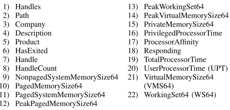
Initially the process details consisted of 64 features (the raw output fromGet-Process | Export-csv, with no specified parameters). However, many of these features were displaying the same information (e.g.,WorkingSet and Work-ingSet64both reported the same memory usage) or deemed to be of little or no value for the purpose of process classification (e.g., FileVersion). After removing duplicate or unnecessary attributes, 22 features were used for the classification model:
1) Handles 2) Path 3) Company 4) Description 5) Product 6) HasExited 7) Handle 8) HandleCount
9) NonpagedSystemMemorySize64 10) PagedMemorySize64
11) PagedSystemMemorySize64 12) PeakPagedMemorySize64
13) PeakWorkingSet64 14) PeakVirtualMemorySize64 15) PrivateMemorySize64 16) PrivilegedProcessorTime 17) ProcessorAffinity 18) Responding 19) TotalProcessorTime 20) UserProcessorTime (UPT) 21) VirtualMemorySize64
(VMS64)
22) WorkingSet64 (WS64)
For each entry,Name was also stored for human readabil-ity and labelling purposes, along with a manually-labelled
Legitimate column, that was used for supervised training. Each process will generate multiple data entries within the same file, with features varying dependant upon the running conditions of the process (e.g., memory usage, running time, etc.). Therefore, a single malware (or benignware) sample could create up to 5000 rows or more of process details (e.g., Table I).
Name Handles Path Company . . . UPT VMS64 WS64
audiodg 109 0 0 . . . 0.0100144 41664512 13869056 audiodg 118 0 0 . . . 0.0100144 41926656 13918208 audiodg 122 0 0 . . . 0.0100144 42450944 13971456 audiodg 122 0 0 . . . 0.0100144 42188800 13959168 2lm5xNQU 80 1 1 . . . 0 50917376 3493888 2lm5xNQU 134 1 1 . . . 0.1702448 61988864 5242880 2lm5xNQU 134 1 1 . . . 0.5407776 63037440 5537792 2lm5xNQU 134 1 1 . . . 0.9413536 63037440 5922816
TABLE I
SAMPLE OF FEATURES TO DESCRIBE PROCESS DETAILS.
[image:2.612.319.554.232.344.2]B. Algorithm Selection and Testing
captured as described previously in Section III-A, along with manual labels for malicious or benign, and then tested against the following classification algorithms:
• Random-Forest
• GNB
• DecisionTree • KNearestNeighbour • AdaBoost
• SVC
[image:3.612.312.568.78.157.2]• GradientBoosting • LogisticRegression • OneClassSVM
Fig. 1. Training and Algorithm Selection Process
We use a k-fold cross validation (k=7) with a testing / validation split of 80 / 20, and feature selection utilised during each run of the comparison script. For each input file this was performed 10 times, giving a total of 100 training runs. A ‘winning’ algorithm was established each time based on the following outputs: Accuracy score, false positive rate and false negative rate. In addition each process was given its own individual score.
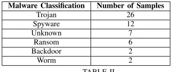
Malware Classification Number of Samples
Trojan 26
Spyware 12
Unknown 7
Ransom 6
Backdoor 2
Worm 2
TABLE II
BREAKDOWN OF MALWARE BY CLASSIFICATION USED IN TRAINING DATA
By the end of the comparison process each algorithm had seen 55 unique malware samples in total (see Table II). Random Forest performed best for this experiment, giving the highest accuracy score for 73 out of 100 training runs (see Table III for the Random Forest accuracy scores). As a result, a Random Forest classifier was then developed and trained using the combined data from all training malware and benignware process, using only the features identified as having been key in 50% or more of the comparison script runs. However, deeper investigation found that the selection of features proved to be inaccurate and would mis-classify benign processes as malware. To overcome this, we performed multiple iterations of feature selection on the combined set
using different feature combinations. We describe the final feature selection in further detail in Section V-A.
Precision Recall F1 False Positive False Negative Runs
1 1 1 <1% <1% 94
1 0.79 0.88 21.41% 0% 1
1 0.97 0.99 2.82% 0% 1
1 0.98 0.99 1.64% 0% 1
1 0.99 0.99 1.29% 0% 1
1 0.99 1 0.92% 0% 2
TABLE III
BREAKDOWN OFCLASSIFICATIONREPORT FORRANDOMFOREST
TRAININGRUNS
C. Live Testing
Following the successful training of the classifier on static data it was then tested live, against previously unseen malware samples. Initially, there was a delay of approximately 30 seconds between a malicious process being started and it being detected by our system. This was deemed unsuitable for the design parameters of desired system.
The classifier was then modified to introduce a whitelisting approach for previously-known processes, such as consistent background processes. The data collection script was also modified to split input files down to a smaller size, limited to the output of 10 iterations of the Get-Processcmdlet. This meant there was a constant creation of new, smaller files, which the system would use as input (see Figure 2). As a result of these modifications the delay was shortened to between 3-8 seconds and deemed to be within acceptable parameters.
Fig. 2. NODENS Live Process
[image:3.612.73.251.454.528.2]the workload for manual interrogation of the data. This also made it more challenging to define which features were key in identifying a malware process.
D. Alternative Classifiers
Two alternative algorithms were trialled during the live testing phase in an attempt to shorten the time between execution and detection. Both a Neural Network and a SGD (Stochastic Gradient Descent) classifier were found to be faster and better suited to incremental learning, however neither were as accurate as the original Random-Forest, with accuracy dropping down to 63% in one instance. The authors believes that in the instance of the Neural Network this drop in accuracy is due to relatively low number of training samples used (the same 55 as used to train the Random-Forest) classifier. It is highly likely that with access to a larger, more industrial scale data-set the accuracy of the Neural Network could be improved. The dataset used by Rhode et al. [7] is publicly available, however we found that the features they provide did not coincide with those that we have identified, making it difficult for comparison. A comparison between the difference feature sets is a potential area for future research.
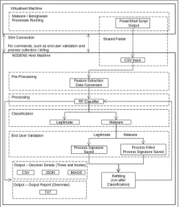
[image:4.612.311.571.50.350.2]E. NODENS
Figure 3 shows an end to end overview of the NODENS work flow. A command line interface was implemented which allows an end user to utilise multiple different ‘plug-in scripts’, such as being able to start and stop the data collection and detection process from the command line, as well the termination of malware processes and re-fitting of the clas-sifier upon identification of previously unseen malware. The classifier would also seek clarification on previously unseen, but suspected malware processes, in this way the classifiers understanding could be refined with the assistance of the end-user and limit the chances of misidentifying processes and then embedding these errors into the algorithm.
The refitting was proven to be effective as it allowed the system to identify malware process it had previously not detected, correctly identifying 5 previously undetected malware processes following refitting. This demonstrates that the system was able to increase it’s understanding of malware processes and points to a generalised link between all malware process behaviour, based off the ability for the system to use readily identified malware and their features to then identify those it had previously missed. We believe that this is linked to the common factors found across the malware samples NODENS was tested against, which we discuss in Section VI. It also demonstrates how an adaptive system such as NODENS can remain at the forefront of malware detection.
IV. DATASET
As described in Section III, malware samples were gath-ered and deployed within a Windows 7 VM using the
Get-Process cmdlet. This gave an initial CSV file that consists of the typical background processes for a Windows 7 VM, the PowerShell process, and the malware process.
Fig. 3. Flow diagram for NODENS
Multiple benignware processes were also set to execute during the testing of NODENS to further refine and test the ability to distinguish between malware and benignware.
Subsequently, the ability to re-fit NODENS was introduced as an additional plugin to allow the system to stay at the edge of malware detection and consistently learn from and adapt to changes in the threat landscape. As re-fitting is a continuous process the dataset used for re-fitting is continual expanding, as more malware and benignware processes are added to it.
A. Data Pre-processing
As the output of theGet-Processcmdlet was a mixture of strings, integers and date-time formats it required data-type conversion before the classifier was able to process it. String values were converted to binary data (1 = present, 0 = no value), with the exception of Has Exited, which was translated as 1 = Exited, -1 = Not Exited, and 0 indicates this field had no value during pre-processing. All other data was converted to either integers or floating point, dependent on which was more appropriate, i.e. measurements in seconds and milliseconds. This process was conducted live and ran parallel to the collection and classification of data from the virtualised environment.
B. Training Data
while the benignware samples consisted of data extracted from native windows background processes. Table IV shows the number of process entries in the data that were labelled as either malware or benignware processes. It should be noted that these do not represent individual malware or benignware samples, but the number of times each type of process was seen, and that multiple processes would belong to the same instance of a malware or benignware sample, albeit with variance in features, such as time on processor or virtual memory size:
Process Classification Number Percentage
Malware 95,191 9%
Benignware 953,384 91%
TABLE IV
BREAKDOWN OF TRAINING DATA USED DURING INITIAL TRAINING
C. Live Testing
In addition to testing against downloaded malware samples (see Table V for the breakdown of samples), the system was also tested against malware created using the Metasploit framework (msfvenom). These tests were conducted to test NODENS ability to detect bespoke malware and malware with persistence. While NODENS was able to successfully detect all malware created with msfvenom, including those with persistence, it was unable to defeat the persistence once detected. It would detect and kill the persistent malicious process the first time it ran, but failed to detect or kill the process if it self-generated a second time. We believe that this is likely tied to the persistence process having a smaller memory footprint on being re-initialised, using cached and recent memory. Detecting of malware persistence would be a further area of research outside the scope of this current work.
Malware Classification Number of Samples Detection Ratio
Trojan 47 93%
Ransom 15 100%
Spyware 15 100%
Backdoor 7 100%
Bit Coin Miner 3 100%
Process Injector 3 100%
Virus 1 100%
TABLE V
BREAKDOWN OF MALWARE CLASSIFICATIONS USED DURING LIVE TESTING OFNODENS,INCLUDING DETECTION RATES
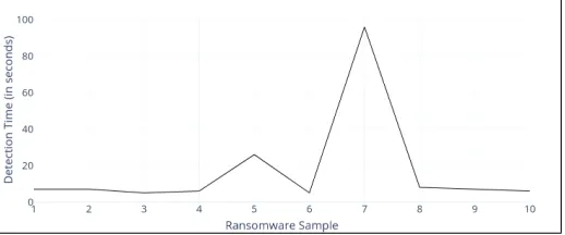
D. Ransomware
Given the current threat landscape, there is a significant shift towards ransomware attacks where a user’s files are encrypted and a payment is demanded (tyipcally via Bitcoin) to decrypt the files to their original state. As an increasingly popular form of attack, it is important to test NODENS against this malware variant. As such a dedicated ransomware test was conducted and recorded using 10 unique samples of ransomware, which were downloaded and executed in the VM environment. On average, NODENS was able to identify the ransomware sam-ples within 9 seconds of execution. However, in one particular
[image:5.612.312.571.261.369.2]case it was noted that NODENS and the ransomware were ‘racing’ each other. This race occurred because the method of data processing meant that there was window of time when the output of the Get-Process cmdlet was accessible to the ransomware on the VM creating a race condition. In certain cases, this meant the CSV file would arrive encrypted and NODENS would be unable to process it, forcing it to wait for the creation of the next CSV file (with a new file being produced every 10 iterations ofGet-Process). In all tested scenarios NODENS was able to identify the ransomware samples, however in this particular example, the encryption of the CSV meant that detection took 96 seconds (see Figure 4). This time frame is obviously outside the design parameters that NODENS was built around. A further consideration for the system would be how to prevent infection or encryption of files that are associated with the detection routines.
Fig. 4. Ransomware Detection
V. INTERPRETABILITY
The interpretability of NODENS originally started as man-ual interrogation of the raw CSV output from the processes, showing which process had been classified as benignware or malware and the values for each process feature. Later on the system was modified to automate the production of decision-specific data as a choice of CSV or different graphical file(s). This made understanding the data and the relevant decision thresholds much easier. This output could be created in one or multiple formats for malware, benignware or both, dependant on end user preference. In the following sections of the paper malware processes are referred to as class 0, this is due to the binary classification nature of processes by the algorithm.
A. Raw Data
During the initial phase, the output from the classifier was manually interrogated. The data consisted of all the processes from each run of NODENS and the feature values. The use of feature selection was important as it helped to filter the size of the output dataset and therefore helped to identify features that were deemed to be key in the identification of malware processes.
The following features were identified as being crucial for the distinction between benignware and ransomware:
• ProcessorAffinity - (Binary Data)
• HandleCount - (Variable Data) • HasExited - (Binary Data)
• Company - (Binary Data)
• Description - (Binary Data)
• PeakVirtualMemorySize64 - (Variable Data)
• TotalProcessorTime - (Variable Data)
• PeakWorkingSet64 - (Variable Data)
• PrivateMemorySize64 - (Variable Data)
• WorkingSet64 - (Variable Data)
• Path - (Binary Data)
From these features those in bold were later also identified as a root node decision points during the decision-specific phase.
B. Decision Specific Data
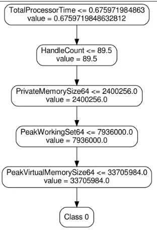
Given the difficulty in interpreting the raw data NODENS was modified to output the decision from each decision tree and subsequent nodes. This is an iterative process run at the point of classification that provides output specific to the end users requirements. Initially output was a CSV file showing which decision trees had classified a process as either malware or benignware, dependent on the end users selection, this included the nodes within those trees and their decision thresholds (see Figure 5). The capability to output a .json files was then included, with each .json file representing a specific decision tree and children nodes, as this allowed for a greater range of graphical uses and presentation options. Finally an option to output both a .png and .dot file (see Figure 6) were included. This provided the greatest use of visual interpretation.
Fig. 5. Original interpretable output was in CSV form, showing the trees that had classified a process as malware and the relevant decision nodes
[image:6.612.362.518.49.277.2]In this way an end user is able to see why a process has been classified as malware, or not, through an easily understandable
Fig. 6. Output from a .dot file, showing the decision path through a malware node
and interrogatable output. This allows an end user to develop an understanding of the process life-cycle of a malware sample individually, or as part of a larger malware family, including common features shared between different malware samples or types.
VI. RESULTS
A. Raw Binary Data
Data was organised based on the values of the binary data features, in this way a comparison could be more easily drawn between them. In general the output of benignware processes were set to either true or false for all binary features. By comparison malware processes showed a significant range, with multiple combinations of binary values being presented by different processes, as illustrated in Table VI.
B. Raw Variable Data
Variable data consisted of integer and float type parameters and the output score that each process was given by the system. A comparison of the variable data showed that benignware processes had on average a higher score, as shown in Ta-ble VII.
Malware Process
Name
Path Company Description Has Exited
Processor Affinity
bot 1 0 0 0 1
webpos 1 0 0 1 0
p.tmp 1 0 1 -1 1
re1608 1 1 1 -1 1
TABLE VI
[image:6.612.57.294.448.655.2]Total output score Lowest Highest Average Malware 27,321,331 554,336,342 196,841,342 Legitimate 184,082,529 816,992,765 377,574,468
TABLE VII
OUTPUT SCORES FORMALWARE ANDBENIGNWARE PROCESSES
However it was difficult to identify a threshold for distinc-tion through manual inspecdistinc-tion of the output data, as there are instances where the scores for malware processes and benign-ware processes were within the same score bracket (between the lowest or highest score for correctly identified benignware processes, hereafter referred to as a score bracket), yet being correctly identified as malware. To research this further data from malware processes that were correctly identified, yet whose output scores put them inside the benignware output scores bracket was compared to benignware processes that they were scored between or closely to.
There was no immediate distinction between them, with neither binary nor variable data showing a clear pattern. The variable data parameters were then individually compared to see if a differential in values would establish a pattern of identification. This showed that the differential between (Peak)WorkingSet64 and PrivateMemorySet64 was negative for some malware processes, but no benignware processes. This showed that malware processes had (on average) a higher amount of private data than shared, something that was not found in the benignware samples tested.
C. Decision Specific Data
The decision specific data allowed the confirmation of conclusions and assessments drawn from manual inspection of raw data, as well as providing greater and more accurate analysis of which features were key in the identification of malware, particularly the thresholds and their frequency as decision points.
The decision specific data was collated together and the common features compared. As would be expected compar-ison of entire random tree decision paths across multiple malware processes was impossible, and decision trees were only comparable to others from different process cycles of the same malware, from within the same run. Therefore comparison was limited to the initial decision points (referred to as root nodes) for each decision tree, as these were the only consistent features across multiple outputs and different malware processes. As shown in Table VIII, 15 root node features and thresholds were identified, though out of these 2 are duplicated features with different thresholds (Paged System Memory Size64 and Handle Count), of these 7 features had been previously identified as key through feature selection and manual inspection of the raw data. These same features were also used throughout the decision trees as later nodes, however the thresholds were varied. Though it is important to note that these root nodes remained unchanged after multiple re-fittings. It was only when altering the value for n_estimators were any changes noted in the root nodes, these primarily being the
threshold values with minimal to no changes in the features used.
Root Node Feature Threshold Frequency
Processor Affinity 0.5 20%
Total Processor Time 0.675971984863 16% User Processor Time 0.625900030136 16%
Handle 186 13%
Path 0.5 12%
Product 0.5 10%
Privileged Processor Time 0.00500719994307 3% Paged System Memory Size64 100756.0 2% Peak Virtual Memory Size64 53284864.0 2%
Handle Count 231.5 1%
Virtual Memory Size64 51525632.0 1% Paged System Memory Size64 100692.0 <1%
Handles 231.5 <1%
Handle Count 204.5 <1%
Working Set 64 19572736.0 < 1% TABLE VIII
ROOT NODE FEATURES,THEIR THRESHOLDS(AS ROOT NODES)AND FREQUENCY OF USE THROUGHOUT THE TESTING OFNODENS
The inclusion of multiple memory orientated features adds weight to previous assessments regarding the unique memory usage foot print that malware process create. Though the private memory feature is not included as a root node, it is used in other nodes as a decision point, which indicates that there are other memory traits beyond the imbalance between private and shared memory which are used to identify the memory footprint of a malware process.
These features are also used infrequently as root nodes, suggesting that the classifier uses other metrics in favour of memory analysis, most common being the malware process affinity and the amount of time it spends running. It is the authors assessment that these features are used due to the number of malware processes which will run for a short period of time before either injecting themselves into a new or already existing process, or removing themselves completely from the system, in an attempt to avoid detection by decreasing their run time and the window of opportunity for current anti-malware systems to detect them. This assessment is backed up by the inclusion and high frequency of the path feature, as such malware processes commonly remove the file used to launch them.
While these behaviours are not universal across all malware, either those seen by NODENS or in general, it does provide an ‘easy win’ for the classifier as these behaviours are not exhibited by benignware processes, which in the authors opinion explains their frequent use as root nodes.
D. Refitting
already detectable malware process signatures. By incorpo-rating what it had been able to detect and understood to be malicious into the classifier it was able to further increase accuracy and understanding of what a malicious process is, which would not be possible if there were no common links between the behaviour of malware processes overall.
VII. LIMITATIONS ANDFUTUREWORK
The biggest limitation for NODENS is the size of the dataset used to date, which is small, consisting of 146 malware samples in total, including the training dataset. This can only be solved though continuous testing of the systems against malware samples or through bulk malware data collection. However it is the authors opinion that the number of process details generated per sample helps offset this limitation.
Another limitation is that all of the training and testing malware samples were run in a virtualised environment, mean-ing that it was not possible to train the system against ‘VM aware’ malware. Whilst a more sophisticated environment could be developed to fool the malware via networking checks, a genuine physical networking environment is required to fully test against VM aware malware.
The current systems use of shared folders for process output and system input would need to be improved upon in future work to make NODENS more robust and remove the current race condition that it faces with ransomware.
VIII. CONCLUSION
The NODENS system has shown that it is possible to create lightweight, accurate and most importantly, interpretable automated malware detection systems.
While the dataset used in the training and testing of both systems are comparatively small, the current accuracy of NODENS and proven ability to refit and identify previously undetected malware processes, shows that the system can remain at the forefront of malware detection and is highly adaptable, a key consideration in the ever changing threat landscape of cyber security.
The in-depth, decision specific interpretability that NODENS offers added weight to assessments drawn from analysis of raw data and makes it easier for future analytical work to be carried out, using easily understandable output formats. This will help increase awareness of both what a malware process is doing on a system and aid in the creation of a generalised malware model for further malware orientated research. Such knowledge will aid in the accuracy of anti-malware systems, allowing both researchers and commercial vendors to hone in on malware specific signatures, such as the potentially unique memory foot print of malware processes identified through NODENS, making it harder for malicious agents to create undetectable malware.
Three metrics for malware distinction were identified, al-lowing for the creation of a malware process model:
• Binary values, particularly the company and description features, were shown to be a reliable metric as they are rarely populated in malware.
However this could change if these features are populated in more malware samples.
• The output score and differential between (Peak)WorkingSet64 and PrivateMemorySet64 were negative for the majority of the malware processes and none of the legitimate processes, as such this could also be used to identify malware processes.
• A comparison between process run time and changes in certain binary values, such as path, provide a clear pattern of behaviour that is not seen in benignware processes, such as the trend for malware processes to remove their own binary files as previously mentioned.
However it is worth noting that none of the above metrics were 100% accurate in isolation. As such an approach that utilises multiple methods of distinction is considered best. It is also the authors opinion that further research is required in the area of machine learning malware detection, with a focus on the identification and distinction features that are used to classify and separate processes.
REFERENCES
[1] D. Ucci, L. Aniello, and R. Baldoni, “Survey of machine learning techniques for malware analysis,” Computers & Security, vol. 81, pp. 123–147, 2019.
[2] “Machine learning for malware detection,” Kaspersky Enterprise Cyber-security, Tech. Rep., 2017.
[3] I. Firdausi, C. Lim, A. Erwin, and S. N. Anto, “Analysis of machine learning techniques used in behavior-based malware detection,” in2010 Second International Conference on Advances in Computing, Control, and Telecommunication Technologies, 2010, pp. 201–203.
[4] R. Tian, R. Islam, L. Batten, and S. Versteeg, “Differentiating malware from cleanware using behavioural analysis,” in2010 5th International Conference on Malicious and Unwanted Software, 2010, pp. 23–30. [5] S. S. Hansen, T. M. T. Larsen, M. Stevanovic, and J. M. Pedersen, “An
approach for detection and family classification of malware based on behavioral analysis,” in2016 International Conference on Computing, Networking and Communications (ICNC), Workshop on Computing, Networking and Communications (CNC), 2016, pp. 1–5.
[6] S. Tobiyama, Y. Yamaguchi, H. Shimada, T. Ikuse, and T. Yagiup, “Malware detection with deep neural network using process behavior,” in2016 IEEE 40th Annual Computer Software and Applications Con-ference, 2016, pp. 577–582.
[7] M. Rhode, P. Burnap, and K. Jones, “Early-stage malware prediction using recurrent neural networks,” Computers & Security, vol. 77, pp. 578–594, 2018.
[8] T. Shibahara, T. Yagi, M. Akiyama, D. Chiba, and T. Yada, “Efficient dynamic malware analysis based on network behavior using deep learn-ing,” in2016 IEEE Global Communications Conference (GLOBECOM), 2016.
[9] J. Saxe and K. Berlin, “Deep neural network based malware detection using two dimensional binary program features,” in2015 10th Interna-tional Conference on Malicious and Unwanted Software (MALWARE), 2015.
[10] R. Pascanu, J. W. Stokest, H. Sanossian, and A. T. Mady Marinescu, “Malware classification with recurrent networks,” in 2015 IEEE In-ternational Conference on Acoustics, Speech and Signal Processing (ICASSP), 2015, pp. 1916–1920.