GNSS and InSAR based water vapor tomography: A Compressive Sensing solution

GNSS and InSAR based water vapor tomography:

A Compressive Sensing solution

Zur Erlangung des akademischen Grades einer

Doktor-Ingenieurin

von der Fakultät

für Bauingenieur-, Geo- und Umweltwissenschaften

des Karlsruher Instituts für Technologie

genehmigte

Dissertation

von

M.Sc. Marion Elsa Amelie Heublein

aus Nürnberg

Tag der mündlichen Prüfung: 22.2.2019

Hauptreferent: Prof. Dr.-Ing. habil. Stefan Hinz

Institut für Photogrammetrie und Fernerkundung

Karlsruher Institut für Technologie

Korreferenten: Dr.-Ing. Uwe Ehret

Institut für Wasser und Gewässerentwicklung – Hydrologie

Karlsruher Institut für Technologie

Prof. Dr.-Ing. habil. Xiaoxiang Zhu

Signal Processing in Earth Observation

Remote Sensing Technology Institute

German Aerospace Center

Abstract

An accurate knowledge of the three-dimensional (3D) distribution of water vapor in the atmosphere is a key el-ement for weather forecasting and climate research. In addition, a precise determination of water vapor is also required for accurate positioning and deformation monitoring using Global Navigation Satellite Systems (GNSS) and Interferometric Synthetic Aperture Radar (InSAR). Several approaches for 3D tomographic water vapor re-construction from GNSS-based Slant Wet Delay (SWD) estimates exist. Yet, due to the usually sparsely distributed GNSS sites and due to the limited number of visible GNSS satellites, the tomographic system usually is ill-posed and needs to be regularized, e.g. by means of geometric constraints that risk to over-smooth the tomographic refractivity estimates.

Therefore, this work develops and analyzes a Compressive Sensing (CS) approach for neutrospheric water vapor tomographies benefiting of the sparsity of the refractivity estimates in an appropriate transform domain as a prior for regularization. The CS solution is developed because it does not include any geometric smoothing constraints as applied in common Least Squares (LSQ) approaches and because the sparse CS solution containing only a few non-zero coefficients may be determined, at a constant number of observations, based on less parameters than the corresponding LSQ solution. In addition to the developed CS solution, this work introduces SWDs obtained from both GNSS and InSAR into the tomographic system in order to dispose of a better spatial distribution of the observations. The novelties of this approach are 1) the use of both absolute GNSS and absolute InSAR SWDs for tomography and 2) the solution of the tomographic system by means of Compressive Sensing. In addition, 3) the quality of the CS reconstruction is compared with the quality of common LSQ approaches to water vapor tomography.

The tomographic reconstruction is performed, on the one hand, based on a real data set using GNSS and InSAR SWDs and, on the other hand, based on three different synthetic SWD data sets generated using wet refractivity information from the Weather Research and Forecasting (WRF) model. Thus, the validation of the achieved re-sults focuses, on the one hand, on radiosonde profiles and, on the other hand, on a comparison of the refractivity estimates with the input WRF refractivities. The real data set resp. the first synthetic data set compares the recon-struction quality of the developed CS approach with LSQ approaches to water vapor tomography and investigates in how far the inclusion of InSAR resp. synthetic InSAR SWDs increases the accuracy and precision of the refrac-tivity estimates. The second synthetic data set is designed in order to analyze the general effect of the observing geometry on the quality of the refractivity estimates. The third synthetic data set places a special focus on the sensibility of the tomographic reconstruction to different numbers of GNSS sites, varying voxel discretization, and different orbit constellations.

In case of the real data set, for both the GNSS only solution and a combined GNSS and InSAR solution, the refractivities estimated by means of the LSQ and CS methodologies show a consistent behavior, although the two solution strategies differ. The synthetic data sets show that CS can yield very precise and accurate results, if an appropriate tomographic setting is chosen. The reconstruction quality mainly depends on i) the accuracy of the functional model relating the SWD estimates to the refractivity parameters and to the distances passed by the rays within the voxels, ii) the number of available GNSS sites, iii) the voxel discretization, and iv) the variety of ray directions introduced into the tomographic system.

The sizes of the study areas associated to the real resp. to the synthetic data sets are about 120×120km2and about 100×100km2_{, respectively. In the real data set, a total of eight GNSS sites is available and SWD estimates of GPS} and InSAR are introduced. In the synthetic data sets, different numbers of sites are defined and a variety of ray directions is tested.

Zusammenfassung

Unvollständig oder ungenau erstellte Modelle atmosphärischer Effekte schränken die Qualität geodätischer Welt-raumverfahren wie GNSS (Globale Satelliten-Navigationssysteme) und InSAR (Interferometrisches Radar mit synthetischer Apertur) ein. Gleichzeitig enthalten Zustandsgrößen der Erdatmosphäre, allen voran die drei-dimensionale (3D) Wasserdampf-Verteilung, wertvolle Informationen für Klimaforschung und Wettervorhersa-ge, welche aus GNSS- oder InSAR-Beobachtungen abgeleitet werden können. Es gibt etliche Verfahren zur 3D-Wasserdampf-Rekonstruktion aus GNSS-basierten feuchten Laufzeitverzögerungen. Aufgrund der meist spärlich verteilten GNSS-Stationen und durch die begrenzte Anzahl sichtbarer GNSS-Satelliten, treten in tomographischen Anwendungen in der Regel jedoch schlecht gestellte Probleme auf, die z.B. über geometrische Zusatzbedingungen regularisiert werden, welche oft glättend auf die Wasserdampf-Schätzungen wirken.

Diese Arbeit entwickelt und analysiert daher einen Ansatz, der auf einer Compressive Sensing (CS) Lösung des to-mographischen Modells beruht. Dieser Ansatz nutzt die Spärlichkeit der Wasserdampf-Verteilung in einem geeig-neten Transformationsbereich zur Regularisierung des schlecht gestellten tomographischen Problems und kommt somit ohne glättende geometrische Zusatzbedingungen aus. Eine weitere Motivation für die Nutzung einer spär-lichen Compressive Sensing Lösung besteht darin, dass die Anzahl an zu bestimmenden von Null verschiede-nen Koeffizienten bei gleichbleibender Anzahl an Beobachtungen in Compressive Sensing geringer sein kann als die Anzahl an zu schätzenden Parametern in üblichen Kleinste Quadrate (LSQ) Ansätzen. Zur Erhöhung der räumlichen Auflösung der Beobachtungen führt diese Arbeit zudem sowohl feuchte Laufzeitverzögerungen aus GNSS als auch aus InSAR in das tomographische Gleichungssystem ein. Die Neuheiten des vorgestellten Ansat-zes sind 1) die Nutzung von sowohl GNSS als auch absoluten InSAR Laufzeitverzögerungen für die tomographi-sche Wasserdampf-Rekonstruktion und 2) die Lösung des tomographitomographi-schen Systems mittels Compressive Sensing. Zudem wird 3) die Qualität der CS-Rekonstruktion mit der Qualität üblicher LSQ-Schätzungen verglichen. Die tomographische Rekonstruktion der durch feuchte Refraktivitäten beschriebenen atmosphärischen Wasserdampf-Verteilung beruht auf der einen Seite auf realen feuchten Laufzeitverzögerungen aus GNSS und InSAR und auf der anderen Seite auf drei verschiedenen synthetischen Datensätzen feuchter Laufzeitverzöge-rungen, die aus Wasserdampf-Simulationen des Weather Research and Forecasting (WRF) Modells abgeleitet wurden. Die Validierung der geschätzten Wasserdampf-Verteilung stützt sich somit zum einen auf Radiosonden-Profile und zum anderen auf einen Vergleich der geschätzten Refraktivitäten mit den WRF Refraktivitäten, die zugleich als Eingangsdaten zur Generierung der synthetischen Laufzeitverzögerungen genutzt werden. Der reale bzw. der erste synthetische Datensatz vergleicht die Rekonstruktionsqualität des entwickelten CS-Ansatzes mit üblichen Kleinste Quadrate Wasserdampf-Schätzungen und untersucht, inwieweit die Nutzung von InSAR Lauf-zeitverzögerungen bzw. von synthetischen InSAR LaufLauf-zeitverzögerungen die Genauigkeit und die Präzision der Wasserdampf-Rekonstruktion erhöht. Der zweite synthetische Datensatz wurde dafür ausgelegt, den allgemeinen Einfluss der Beobachtungsgeometrie auf die Refraktivitätsschätzungen zu analysieren. Der dritte synthetische Da-tensatz untersucht insbesondere die Empfindlichkeit der tomographischen Rekonstruktion gegenüber variierenden GNSS-Stationszahlen, unterschiedlichen Voxel-Diskretisierungen und verschiedenen Orbit-Konstellationen. Im realen Datensatz verhalten sich die Kleinste Quadrate Schätzung und der Compressive Sensing Ansatz sowohl für die reine GNSS-Lösung als auch für die kombinierte GNSS- und InSAR-Lösung konsistent. Die synthetischen Datensätze zeigen, dass Compressive Sensing in geeigneten Szenarien sehr genaue und präzise Ergebnisse liefern kann. Die Qualität der Wasserdampf-Schätzungen hängt in erster Linie ab i) von der Genauigkeit des funktionalen Modells, das die feuchten Laufzeitverzögerungen, die zu schätzenden Refraktivitäten und die von den Strahlen in den Voxeln zurückgelegten Distanzen in Beziehung zueinander setzt, ii) von der Anzahl verfügbarer GNSS-Stationen, iii) von der Voxel-Diskretisierung, und iv) von der Vielseitigkeit der in das tomographische System eingebauten Strahlrichtungen.

Die mittels des realen Datensatzes bzw. mittels der synthetischen Datensätze untersuchten Regionen sind etwa 120×120km2 bzw. 100×100km2 groß. Im realen Datensatz stehen acht GNSS-Stationen zur Verfügung und es werden feuchte Laufzeitverzögerungen von GPS InSAR genutzt. In den synthetischen Datensätzen werden unterschiedliche Stationsanzahlen definiert und vielseitige Strahlrichtungen getestet.

Contents

1 Introduction 1

1.1 Relevance of determining the 3D atmospheric water vapor distribution . . . 1

1.2 Relevance of the innovations in the proposed approach . . . 2

1.3 Objectives . . . 3

1.4 Contributions . . . 4

1.5 Outline . . . 4

2 The Earth’s atmosphere: physical foundations and measurement techniques 7 2.1 The Earth’s atmosphere . . . 8

2.1.1 Ionosphere . . . 8

2.1.2 Neutrosphere . . . 9

2.2 Meteorological quantities describing the neutrospheric water vapor distribution . . . 9

2.3 Numerical weather models . . . 12

2.4 Measurement techniques quantifying the neutrospheric water vapor content . . . 13

2.5 Interactions of radio waves and the neutrosphere . . . 16

2.6 Path delay modeling in GNSS and InSAR . . . 17

2.6.1 Modeling the hydrostatic component of the delay using surface meteorology . . . 17

2.6.2 Determining the wet component of the delay content using GNSS PPP . . . 19

2.6.3 Determining the wet component of the delay using PS-InSAR . . . 20

2.7 Summary . . . 22

3 State of the art in tomographic water vapor reconstruction 23 4 Tomographic model 29 4.1 Tomographic equation within a discretized refractivity field . . . 30

4.2 Side rays for better vertical resolution . . . 31

4.3 Effects of the voxel discretization . . . 32

4.4 Raytracing on the ellipsoid . . . 35

5 Methodology for 3D tomographic reconstruction 41 5.1 Mathematical basics for the solution of inverse problems . . . 41

5.2 L2solution vs.L1solution to an inverse problem . . . 44

5.3 Constrained Least Squares solution . . . 46

5.4 Sparse Compressive Sensing solution . . . 50

5.4.1 Sparse dictionaries using Kronecker bases . . . 51

5.4.2 Application of CS to the tomographic reconstruction of atmospheric water vapor . . . 53

5.5 Summary . . . 57

6 Study areas and data sets 59 6.1 Study areas . . . 60

6.2 Real data set . . . 61

6.2.1 GNSS data availability . . . 61

6.2.2 InSAR: data availability, PSI processing, and absolute InSAR ZWD generation . . . 62

Contents

6.2.4 Radiosonde data . . . 63

6.2.5 Real SWD data set based on GNSS and InSAR . . . 65

6.3 Synthetic data set . . . 68

6.3.1 WRF data set . . . 68

6.3.2 Synthetic SWD data set based on WRF . . . 69

6.4 Geodetic and meteorological height systems . . . 70

6.5 Summary . . . 73

7 Tomography results 75 7.1 Real data set . . . 77

7.1.1 Tomographic settings in the real data set . . . 77

7.1.2 Consistency of GNSS, InSAR, and radiosondes . . . 79

7.1.3 Validation of GNSS and InSAR based wet refractivities from CS and LSQ using ra-diosonde profiles . . . 80

7.2 Synthetic data set . . . 82

7.2.1 Synthetic data set comparable to real data set . . . 82

7.2.2 Effect of the observing geometry on the tomographic results within a general study area . 86 7.2.3 Effect of the orbits and of the voxel discretization in a specific study area . . . 99

7.2.4 Summary . . . 107

8 Discussion and Outlook 111 A Appendices 117 A.1 Niell mapping function . . . 117

A.2 PPP processing in Bernese GPS Software 5.2 . . . 117

1 Introduction

An accurate knowledge of the three dimensional (3D) distribution of water vapor in the atmosphere is a key element for weather forecasting and climate research. Moreover, atmospheric water vapor causes a delay in the microwave signal propagation. Thus, a precise determination of water vapor is required for accurate positioning and deformation monitoring using Global Navigation Satellite Systems (GNSS) and Interferometric Synthetic Aperture Radar (SAR) (InSAR). Yet, due to its high variability in time and space, the atmospheric water vapor distribution is difficult to model. This work therefore meets the challenge of tomographically reconstructing the 3D water vapor field by means of developing an innovative Compressive Sensing (CS) solution that includes both GNSS and InSAR observations. The CS solution is motivated by the fact that it does not include any geometric smoothing constraints as applied in common Least Squares (LSQ) approaches and by the fact that the sparse CS solution containing only a few non-zero coefficients may be determined, at a constant number of observations, based on fewer parameters than the corresponding LSQ solution. Within this work, the developed CS approach is compared to common LSQ solution strategies to water vapor tomography. The following details the relevance of an accurate determination of the 3D water vapor field for meteorology, climatology, and space geodesy. Thereafter, a motivation is given for the proposed CS approach using both GNSS and InSAR and for the analysis of the observing geometry’s effect on the quality of the tomographic reconstruction. Finally, the goals and the contributions of this work are summarized and an outline of the thesis is given.

1.1 Relevance of determining the 3D atmospheric water vapor

distribution

As water vapor is a necessary precondition to rainfall, it is important to accurately determine the 3D water vapor distribution in the atmosphere. According to Tuller [1973], the air has to be saturated with water vapor in order to form precipitation. Saturation is reached if the relative humidity RH attains 100%. If RH=100%, an air parcel is saturated with water vapor. Given a constant temperature, it is not possible to add any further water vapor to such a saturated air parcel. E.g. at a temperature of 30◦_{C and a pressure of 1bar, 1kg of air can hold about 26g of}

water vapor. Following the Clausius-Clapeyron equation describing the relationship between the saturation vapor pressure and the air temperature, the relative humidity increases if the water vapor density increases at a constant temperature or if the temperature decreases. Therefore, one key mechanism for attaining saturated air is a decrease in temperature, which may e.g. be reached by means of lifting the air parcel to higher altitudes as at the foot of mountains. Consequently, the windward side of a mountain range usually disposes of more precipitation than the lee side of the same mountain range. At the altitude at which RH=100%, clouds are generated.

However, water vapor only represents a necessary condition to rainfall. Water vapor does not correspond to a sufficient condition for the formation of rainfall. Besides the saturation of air with water vapor, condensation nuclei are necessary in order to form precipitation and the saturated air needs to condense on these particles in order to let grow the water droplets that, if the prevalent buoyant force and updraft is overcome by the weight of the droplets, fall down as precipitation. Condensation nuclei may e.g. originate from products of combustion, oxides of nitrogen, aerosols, or salt particles. According to Park [1999] and Xin and Reuter [1996], the low level water vapor content regulates the timing and the persistence of clouds and moisture convergence below the clouds and the timing and the quantity of rainfall. Thus, variations in the atmospheric water vapor content can cause significant changes in convective rainfall. A 1% moisture variation within a storm cell significantly affects

the storm intensity. Park and Droegemeier [2000] showed the effect of in-cloud moisture on the generation of secondary storm cells and the role of environmental moisture in strengthening a main storm cell. In addition, Stull [2016] states that storms get much of their energy from water vapor and that the amount of precipitation within a storm depends on the amount of moisture in the storm.

Besides its importance as a precondition to rainfall, water vapor corresponds to an important factor within the hydrological cycle. As stated in Mockler [1995], water vapor moves quickly through the atmosphere and redis-tributes energy associated with its evaporation and recondensation. In the case of evaporation, energy is taken up from the surroundings and the environment is cooled, analogously to the cooling effect of a sweating human body. When water vapor condenses, it releases energy and warms the environment. These heat exchanges influence the climate, and thus, good observations of the atmospheric water vapor are essential for understanding climatological processes.

In addition, an accurate knowledge of the 3D water vapor field is crucial for climatology, because water vapor is the most important natural greenhouse gas. According to Bowman [1990], without the natural greenhouse effect, the Earth’s average temperature would be around 30◦_{C lower than it is now. However, in contrast to the}

non-condensable or long-living greenhouse gases like CO2, methane, N2O, and halocarbons, atmospheric water vapor and clouds do not represent drivers of the greenhouse effect but act as fast feedbacks. I.e. water vapor reacts rapidly on changes in temperature, e.g. by evaporation, condensation, or precipitation. In case of anthropogenic emissions of CO2, methane, and other gases causing a rise in temperature, the evaporation rates and thus the atmospheric water vapor density is increased. The increased amount of water vapor, in turn, acts again as a greenhouse gas, absorbs energy that would otherwise escape to space, and so causes additional warming.

Finally, water vapor is an important error source in spaceborne GNSS and InSAR processing. In both techniques, radio wave signals are emitted by the satellite. On their way to the receiver on the ground resp. to the backscattering surface of the Earth (and back to the satellite, in the case of InSAR), these radio wave signals travel through the atmosphere and are delayed by the neutrospheric water vapor. As the neutrospheric water vapor distribution is highly variable both in time and space, the delays caused by water vapor are difficult to correct, when aiming at e.g. geodetic positioning or deformation modeling resp. surface movement applications in GNSS, or at e.g. topographic or deformation applications in InSAR. When compared to the dispersive ionospheric delay accelerating the signal propagation, the wet delay due to water vapor is much smaller but much more difficult to handle, as it cannot be corrected or modeled by multi-frequency measurements. According to Rothacher [2002], the neutrospheric delay in GNSS is highly correlated with the site height and with the receiver clock correction. Therefore it significantly affects the vertical component of the positioning and its effect on the site height needs to be reduced when aiming at precise positioning applications. Concerning InSAR, Zebker et al. [1997] state that the effects of water vapor are larger in magnitude and less evenly distributed throughout the interferogram than neutrospheric variations caused by pressure and temperature changes. Pressure variations typically cause 1.0 to 1.5mbar root mean square pressure variabilities in temperate regions, where a 1mbar pressure change leads to a delay change of about 2.3mm. In contrast, Zebker et al. [1997] report phase changes due to neutrospheric water vapor corresponding to a delay of up to 30cm. When translating these humidity variations into final deformation or topography products, according to Zebker et al. [1997], changes of 20% in relative humidity lead to 10cm errors in deformation products and perhaps 100m of error in topographic maps for pass pairs with unfavorable baseline geometries.

1.2 Relevance of the innovations in the proposed approach

In contrast to existing water vapor tomography approaches usually based on GNSS Slant Wet Delay (SWD) esti-mates only, this work also includes absolute wet delays obtained from InSAR. The inclusion of InSAR SWDs is relevant, because the profile-wise GNSS observations are, in general, sparsely distributed over the study area. This causes, especially in low atmospheric layers, a very low spatial resolution of the observations, which corresponds approximately to the inter-site distance of the GNSS sites of some tens of kilometers. Due to this poor spatial resolution of the GNSS rays in the lowest tomographic layers, the tomographic system of equations is ill-posed

and needs to be regularized. Including area wide InSAR SWDs may help to improve the observing geometry such that the observations are more evenly distributed.

Moreover, thanks to the launch of modern SAR missions such as Environmental Satellite (Envisat), TerraSAR, CosmoSkymed, or Sentinel-1, activities of Persistent Scatterer Interferometry (PSI) increased a lot. As stated in Hansen and Yu [2001], Parker [2017], or Tang et al. [2016], during PSI processing, the atmospheric phase screen can be estimated over wide areas at a temporal resolution of up to six days. Consequently, InSAR can be considered as a valuable resource for water vapor research and should be included within tomographic water vapor reconstructions.

When compared to previous research in the field of water vapor tomography, which is often based on LSQ, a CS solution approach is developed within this work. As in the case of the inclusion of InSAR data into the tomographic system, the use of CS is also motivated by the fact that the tomographic system of equations is ill-posed and needs to be regularized. The regularization can be performed e.g. by including additional observations (as those from InSAR or from surface meteorology) or by imposing constraints on the solution. Yet, the geometric smoothing constraints typically introduced within a LSQ solution to the tomographic system of equations showed to impose unnatural behavior to the water vapor distribution. Therefore, research on alternative regularization schemes is required. Based on the assumption that the signal can be sparsely represented in some appropriate transform domain, CS exploits the sparsity of the transformed water vapor signal for regularizing the tomographic system.

Finally, a reasonable discretization of the analyzed atmospheric volume into volumetric pixels (voxels) of constant water vapor content is essential for most water vapor tomography approaches. Independently of the choice of a LSQ or a CS reconstruction algorithm, the observing geometry, composed e.g. of the satellite positions, the GNSS site distribution, and the voxel discretization should be carefully chosen in order to enable a meaningful solution to the tomographic system. If too few observations are available in order to reconstruct the water vapor distribution at the chosen spatial resolution, or if these observations are too unevenly distributed, the applied constraints may falsify the solution and feign a much higher resolved, but unrealistic solution. This research emphasizes the importance of appropriate voxel sizes for accurately reconstructing the 3D water vapor field.

1.3 Objectives

This thesis aims at developing and analyzing a CS solution to tomographic water vapor reconstructions based on GNSS SWD estimates. In addition, an approach for including InSAR SWD estimates into the tomographic system is proposed. When comparing the reconstruction qualities of the LSQ and the CS solution strategy to the tomographic model, the thesis specially focuses on the questions i) which solution approach is more accurate and more precise, ii) in how far one of the strategies is more flexible, i.e. less constraint-driven, and iii) if the CS solution can do with fewer observations than LSQ. Alternatively, question iii) investigates in how far CS is able to estimate the neutrospheric water vapor field at a higher spatial resolution than LSQ, or if CS can estimate the water vapor field more accurately and more precisely than LSQ, given a certain number of observations and a certain spatial resolution. The influence of the observing geometry on the tomographic results is investigated by means of first analyzing the effect of the number of GNSS sites and of their horizontal distribution within the considered study area on the accuracy and on the precision of the tomographic results. This includes the questions i) if the site distributions should differ in different latitudes and ii) if the sites should be randomly distributed within the analyzed study area or rather situated along a regular grid. In addition, the effect of the ray geometry and of the voxel discretization on the tomographic results is investigated. This is done by means of focusing on the question in how far the inclusion of rays of more satellites than given by the Global Positioning System (GPS) orbits improves the repeatability of the results and by means of investigating how large the tomographic voxels should be in order to yield repeatable results within a changing orbit geometry.

1.4 Contributions

This thesis presents CS as a powerful tool for accurately reconstructing the 3D water vapor field. The sparsity of the water vapor field in an inverse Discrete Cosine Transform (iDCT) Euler Dirac transform domain is shown to be able to serve as a prior for regularizing the ill-posed system of equations encountered in the tomographic reconstruction of water vapor. Moreover, the capacity of InSAR SWD estimates to regularize the tomographic system resp. to improve the accuracy of the tomographic water vapor reconstruction is tested. Finally, the differences between the proposed CS approach and common LSQ approaches resp. between GNSS only resp. GNSS and InSAR solutions to water vapor tomography are analyzed. The thesis shows that, in the case of a CS solution, the observing geometry is of particular importance for the accurate determination of the 3D water vapor field based on profile wise SWD estimates. Moreover, the thesis points out the relevance of carefully selecting the size of the tomographic voxels and investigates the effect of the exact horizontal position of the GNSS sites on the accuracy and on the precision of the tomographic results. The developed tomography approach is based on geometrical and physical models that allow to combining and evaluating very different observation types and measurement techniques at a time. Therefore, the tomography approach represents a very flexible tool, especially under the light of new and heterogeneous satellite missions.

1.5 Outline

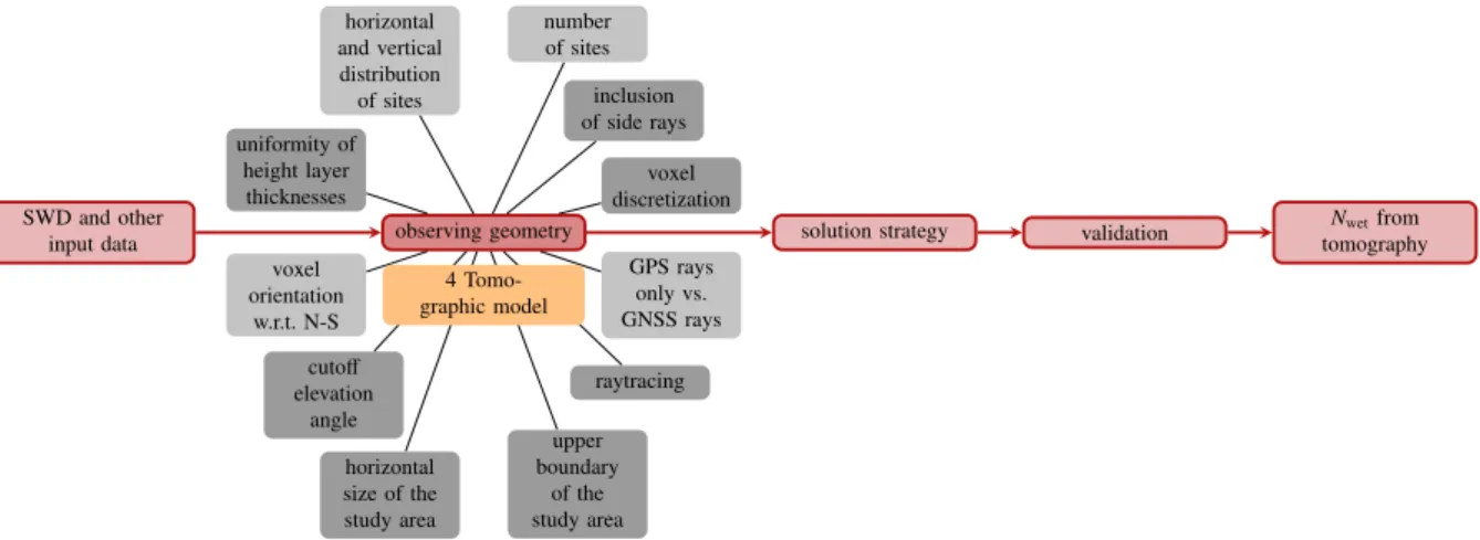
Many aspects need to be taken into account within a tomographic reconstruction of the 3D water vapor field. Therefore, Figure 1.1 shows an advance organizer illustrating the steps yielding 3D water vapor estimates based on e.g. slant wet delay input data. In the case of real data sets, common approaches to water vapor tomography mainly refer on input observations from GNSS and from surface meteorology. If available, e.g. InSAR SWD estimates and observations of Light Detection And Ranging (LiDAR) sensors, microwave radiometers, Very Long Baseline Interferometry (VLBI), radiosondes, or imaging spectrometers may be added. In contrast, in the case of synthetic data sets, the input SWDs are commonly deduced from meteorological quantities like temperature, pressure, and water vapor mixing ratio simulated by Numerical Weather Models (NWM).

In general, the available input data automatically define the number and the spatial distribution of the GNSS sites introduced within the tomographic system. Yet, many other components of the observing geometry need to be defined by the user, e.g. the horizontal size of the study area as well as its upper boundary, the horizontal voxel discretization as well as the thickness of the voxels and their orientation w.r.t. the North-South direction, the cutoff elevation angle for the introduced GNSS rays, the decision for GPS observations only or for GNSS observations, and the inclusion of rays entering the study area only on its top resp. also at the side.

Once the observing geometry settings are defined, a solution strategy can be selected. In this work, LSQ and CS solution approaches are distinguished for the determination of the 3D water vapor distribution. The validation of water vapor distributions estimated based on real data is carried out based on independent data sets that are not yet introduced within the tomographic system. In the case of synthetic data sets, a 3D validation of the estimated water vapor field is possible based on the simulations of e.g. temperatureT, pressurep, and water vapor mixing ratiowvresulting from NWM.

The main steps from the SWD input data to the interpretation of the tomography solution include the definition of the tomographic model according to the available data sets and the associated observing geometry, choosing a solution strategy, and validating the estimated 3D water vapor field. For each of these main steps, the advance organizer in Figure 1.1 indicates which section of this thesis describes resp. analyzes the respective step. In order to better guide the reader through the thesis, selected parts of the advance organizer will reappear at the beginning of the sections corresponding to the main steps of the tomographic reconstruction of the 3D water vapor field. The aspects relevant within the respective sections will then be highlighted within the advance organizer.

SWD and other

input data observing geometry solution strategy validation

Nwetfrom tomography real data set

ZTDs from GNSS ZDDs from surface meteorology additional data sets InSAR LiDAR microwave radiometers surface meteorology radiosondes imaging spectro-meters, e.g. MERIS VLBI

synthetic data set numerical weather models, e.g. WRF wv p T observations integrated along ray path

observations from coarse resp. fine voxel discretization number of sites voxel discretization inclusion of side rays horizontal and vertical distribution of sites uniformity of height layer thicknesses horizontal size of the study area GPS rays only vs. GNSS rays upper boundary of the study area cutoff elevation angle voxel orientation w.r.t. N-S raytracing LSQ QCSQ smoothing

constraints knowledgeprior e.g. surface meteorology trade-off: data driven vs. model based terms dictionary

not yet used, independent additional data sets

numerical weather models, e.g. WRF InSAR LiDAR microwave radiometers surface meteorology radiosondes imaging spectro-meters, e.g. MERIS GNSS VLBI

2 The Earth’s atmosphere: physical foundations and measurement techniques

2 The Earth’s atmosphere: physical foundations and measurement techniques

6 Study areas and data sets

6 Study areas and data sets

4 Tomo-graphic model

5 Methodology for 3D tomographic

reconstruction 7 Tomographyresults 7 Tomography

results

Figure 1.1:Advance organizer illustrating the steps yielding 3D water vapor estimatesNwetbased on the input slant wet delay observations. The figure shall give an overview over the main steps of a water vapor tomography illustrated in red. In this way, the advance organizer shall prepare the reader to more efficiently handle and to better understand the thesis. At any one time that one of the steps is explained or investigated within the thesis, the advance organizer will appear and the respective step will be highlighted. For each of the main steps shown in red, relevant aspects effecting the respective step of the tomographic reconstruction are summarized within the advance organizer. Blue colors refer to the case of a tomographic reconstruction of water vapor using real data, whereas green colors stand for synthetic data. Gray colors are relevant for both real and

2 The Earth’s atmosphere: physical foundations

and measurement techniques

Tomographic water vapor modeling with space geodetic techniques like GNSS and InSAR necessitates a good understanding of the atmosphere’s structure, of measurement techniques quantifying the water vapor distribution, and of interactions of electromagnetic waves with the atmosphere. Therefore, this chapter first gives an overview over the Earth’s atmosphere and its common subdivision w.r.t. the temperature profile resp. w.r.t. the plasma den-sity in Section 2.1. When subdividing the atmosphere according to the prevailing plasma denden-sity, the two main horizontal layersneutrosphereandionosphereare distinguished. In this work, the focus is set on the electrically neutral lower≈10km of the atmosphere, the neutrosphere, in which most of the atmospheric water vapor resides. Therefore, Section 2.2 introduces meteorological quantities describing the neutrospheric water vapor distribution. The meteorological quantities are crucial for understanding the relation between the profile-wise SWD input data to water vapor tomography and the 3D water vapor field that shall be tomographically reconstructed. As illustrated in Figure 2.1, this work relies on both a real data set and synthetic data sets. The synthetic data sets are based on simulations of the Weather Research and Forecasting Model (WRF) model. Thus, Section 2.3 generally explains the modeling of the atmospheric state in NWMs for the synthetic data sets, and Section 2.4 presents, for the real data set, both meteorological and geodetic measurement techniques quantifying the neutrospheric water vapor con-tent. Since radio waves and the neutrosphere interact, GNSS and InSAR radio wave observations can be used for water vapor tomography (Section 2.5). The GNSS and InSAR path delay modeling is explained in Section 2.6. In the case of InSAR, a special focus is set on illustrating how absolute wet delays per Persistent Scatterer (PS) can be obtained based on the temporally differentiated, short-wavelength water vapor signal observed as the InSAR atmospheric phase.

SWD and other

input data observing geometry solution strategy validation tomographyNwetfrom real data set

ZTDs from GNSS ZDDs from surface meteorology additional data sets InSAR LiDAR microwave radiometers surface meteorology radiosondes imaging spectro-meters, e.g. MERIS VLBI

synthetic data set numerical weather models, e.g. WRF

wv

p T 2 The Earth’s

atmo-sphere: physical foundations and measurement techniques

2 The Earth’s atmo-sphere: physical foundations and measurement techniques

Figure 2.1: Water vapor tomographies aim at reconstructing the 3D water vapor fieldNwet based on e.g. slant wet delay input data. In the case of real data, such SWD input data can e.g. be derived from GNSS, InSAR, and surface meteorological information. Alternatively, in synthetic data sets deduced from numerical weather models, the SWD input information to tomography is commonly deduced from meteorological quantities like pressurep, temperatureT, and water vapor mixing ratioswv.

2.1 The Earth’s atmosphere

The Earth’s atmosphere can be structured into different layers by means of, e.g. considering the prevailing temper-ature profile or the plasma density. Figure 2.2 shows these two subdivisions of the atmosphere. When considering the subdivision of the atmosphere with respect to the prevailing temperature profile, the lowest layer, extending from the Earth’s surface up to the first temperature minimum, is calledtroposphere. In contrast, from the per-spective of the ionization of the atmosphere, the lowest layer is calledneutrosphere, followed, in higher altitudes, by theionosphere. As stated in Kelley [2009], due to the pervasive influence of gravity, the neutrosphere and the ionosphere are to first order horizontally stratified. In this work, the focus is set on the non-ionized atmospheric regions, especially on the lowest 10km of the neutrosphere, containing a large amount of the atmospheric water vapor. Therefore, the termneutrosphereis preferred to the termtropospherein this thesis. The following two subsections give a short overview over the ionosphere and the neutrosphere.

Neutral gas Mesosphere Stratosphere Troposphere Thermosphere Ionized gas Protonosphere F8Region E8Region D8Region Altitude8N kmI Altitude8N kmI 1000 100 10 1 1000 100 10 1 0 400 800 1200 1600 103 104 105 106 Temperature8in8K Plasma8density8in8cm3 Day Night Neutrosphere Ionosphere

Figure 2.2: Typical profiles of atmospheric temperature and ionospheric plasma density according to Kelley [2009]. On the left, the various layers are distinguished by means of their temperature. On the right, the dif-ferent layers are characterized by their ionization. The termsionosphereandneutrospherein blue were added to the figure from Kelley [2009].

2.1.1 Ionosphere

League [1997] describes the ionosphere, starting at a height of about 60km above the Earth’s surface, as a region in which the air pressure is so low that free electrons and ions can move for a while without getting close enough to recombine into neutral atoms. The ionization is mainly caused by the ultraviolet solar radiation in the outer regions of the atmosphere. However, the ionization does not uniformly increase with the distance from the Earth’s surface. Instead, there are different layers of high ionization at well-defined heights between about 40km to 300km above the Earth’s surface. As the effect of the ionosphere on radio wave signals is related to the time of day, the season of the year, and variations in the solar activity characterized by the sunspot number, the intensity of the ionization within each layer and the exact layer heights vary over time. For the last two decades, Figure 2.3 exemplary shows that maximum sunspot numbers are observed at a repeat cycle of about eleven years. This repeat cycle is superposed by an 80 to 100 years super cycle.

19900 1995 2000 2005 2010 2015 100 200 300 Year Sunspot number Observed Smoothed

Figure 2.3:Sunspot numbers of the last decades based on data from the American National Oceanic and Atmo-spheric Administration (NOAA) Space Weather Prediction Centerftp://ftp.swpc.noaa.gov/pub/weekly/ RecentIndices.txt(09.07.2018).

In addition, as the ionosphere is a dispersive medium, the ionospheric delay on radio wave signals depends on the signal’s frequency. Thus, as described in Hofmann-Wellenhof et al. [2008], multi frequency measurements enable a significant reduction of the ionospheric effect on the GNSS signal propagation time. Böhm and Schuh [2013] relate various GPS first-order measured parameters and the Total Electron Content (TEC) of the Earth’s ionosphere. E.g. they state that a 1.000m range error, i.e. a delay of 3ns, is caused by an electron content of 6.15×1016_el/m2 resp. of 3.73×1016_el/m2_{at the GPS frequencies f1 resp. at f2. In the case of InSAR, the ionospheric delay,} however, is not corrected by dual frequency measurements. Thanks to the small wavelength of about 6cm in the case of C-band SAR observations and because of the low solar activity around the data acquisitions in 2005, the ionospheric delay on InSAR as well as the Faraday rotation significant at L-band or lower frequencies (Jehle et al. [2005]) are neglected in this work.

2.1.2 Neutrosphere

According to Caballero [2014], the neutrosphere can be considered, to an excellent approximation, as a two com-ponent gas consisting of variable proportions of dry air and water vapor. Curry and Webster [1999] state that “water vapor is the most important gas in the atmosphere from a thermodynamic point of view because of its ra-diative properties as well as its ability to condense under atmospheric conditions”. Water is the only atmospheric constituent that attains all three phases – gaseous, liquid, and solid – at the typical pressures and temperatures experienced in the Earth’s atmosphere. According to Seidel [2002], nearly half of the atmospheric water vapor re-sides in the lowest 1.5km of the atmosphere, and less than 5% are contained above 5km. Radiosonde observations have shown that the water vapor content in heights above about 10km is negligible in the study areas considered within this research.

2.2 Meteorological quantities describing the neutrospheric water vapor

distribution

In order to get a better understanding of the both temporally and spatially highly variable neutrospheric water vapor distribution and the relation between water vapor, temperature, and humidity, this section introduces several meteorological quantities describing the neutrospheric water vapor field. The introduced quantities are essential

for relating the tomography input SWDs to the 3D water vapor field. According to Stull [2016], the 3D water vapor distribution can e.g. be expressed by the water vapor mixing ratio

wv=mwatervapor

mdryair , (2.1)

which is commonly given in g/kg because the mass of water vapormwatervaporwithin the air is much smaller than the mass of dry airmdryair. Alternatively, the neutrospheric water vapor distribution can be described by the specific humidityqv, also commonly given in g/kg,

qv=1000·₁wvin kg/kg +wvin kg/kg=

mwatervaporin g

mtotalairin kg , (2.2)

which can be related to the 3D water vapor field by solving

qv=

0_·e

p−e(1−0) (2.3)

from Stull [2016] for the partial pressureein hPa of water vapor:

e= qv·p

0+qv·(1−0) (2.4)

In the Equations 2.3 and 2.4,pin hPa is the atmospheric pressure and the ratio between the gas constant of dry air and the gas constant of pure water vapor0=0.622 is used. The factor 0.622=18/29 corresponds to the ratio of the molecular masses of water and air.

Finally, the 3D water vapor distribution can also be described by the wet refractivity fieldNwet. The term

refrac-tivitywill be explained in more detail in Section 2.5. According to Bevis et al. [1992],Nwet in ppm, with ppm standing for mm/km, is related to the partial pressure of water vaporein hPa and to the temperatureT in K as follows: Nwetin ppm=k0₂·e T+k3· e T2 (2.5) with k0 2=k2−k1·M_Mwatervapor dryair , (2.6)

from Davis et al. [1985], where the constantsMwatervapor=18.0153g/mol and Mdryair=28.9647g/mol in Equa-tion 2.6 are the molar masses of water vapor and of dry air. The constant factorsk1,k2, andk3are given in Smith and Weintraub [1953] as:

k1 = 77.6K/hPa k2 = 72K/hPa k3 = 3.75·105_K2_/hPa

(2.7)

Besides Smith and Weintraub [1953], many research on the refractive indices was carried out. Therefore, Rüeger [2002] summarizes the developments in refractive index equations for radio wave and millimeter waves over the years 1970 to 2000. In Table 2.1, typical values forqvandefrom Stull [2016] as well as the corresponding wet refractivities computed using Equation 2.5 are given for a pressure ofp=1013.25hPa.

Table 2.1:Typical values ofqvandeat a pressure ofp=1013.25hPa.

T in◦_{C qvin g/kg ein hPa Nwetin ppm} −10 1.7666 2.875 15.8284 −5 2.5956 4.222 22.3923 0 3.7611 6.113 31.2556 5 5.3795 8.735 43.0839 10 7.6005 12.320 58.6574 10

If the dew point temperatureTdand the temperatureT are given instead of the partial pressure of water vapor, the value ofecan be derived from the relative humidity RH and the temperature, divided by Kelvin, using

e= RH 100·exp

−37.2465+0.2131665·T−0.000256908·T2

(2.8) from Xu and Xu [2007]. Lawrence [2005] state that the relative humidity can be computed based on the tempera-ture and the dew point temperatempera-ture, both divided by Kelvin, by means of

RH=100₋5_·(T₋T_d). (2.9)

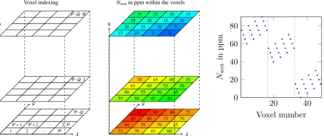
IntegratingNwetalong theith slant ray path spiwith differential dlyields the observation equation for the SWDi,cont along that path

SWDi,cont(in m)=10−6· Z

spi

Nwet(in ppm)dl(in m), (2.10)

or the observation equation for SWDi,discalong discretized segmentsdi jof the slant ray path in mm instead of m SWDi,disc(in mm)=

L X

j=1

Nwetj(in ppm)·di j(in km). (2.11)

As illustrated in Figure 2.4, the variabledi jcorresponds to the distance passed by the slant ray pathiwithin voxel j, andLis the total number of voxels within some tomographic grid.

rayi

di j

Nwet j

Figure 2.4:Ray crossing the tomographic voxel grid.

In addition, the 3D wet refractivity field can be related to further integrated quantities like the Precipitable Wa-ter (PW), the Integrated WaWa-ter Vapor (IWV), or the Zenith Wet Delay (ZWD) as indicated in Figure 2.5. The discretized formula for obtaining PW is given in the following equation:

PW (in mm)= L X

j=1

qvj (in g/kg)·ρ·dzenith,j(in km) (2.12) wheredzenith,j represents the distance passed by the zenith ray path crossing the voxel j, andρ=1 g/cm3is the density of water.

According to Bevis et al. [1992], the precipitable water is related to the integrated water vapor in the zenith direction (IWVzenith_{) and to the ZWD as follows}

PW=IWV

zenith

ρ =Π·ZWD (2.13)

and the conversion factorsQandΠ

Q=0.1022+1708.08 Tmin K =

1

between delays and IWV and its inverseΠcan be approximated using

Tm≈70.2+0.72·T0 (2.15)

for the computation of the neutrospheric mean temperatureTmbased on the surface temperatureT0in K. Alshawaf [2013] analyzed the sensitivity ofQw.r.t. to the surface temperature.

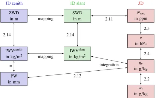
Figure 2.5 summarizes the relation between GNSS or InSAR integrated wet delays or precipitable water and the 3D water vapor mixing ratios simulated by the WRF model. The figure shows the relation between one dimensional (1D) wet delay input data to tomography and the 3D wet refractivity field Nwet to be estimated. In addition, related 1D quantities like the precipitable water or the integrated water vapor as well as related 3D quantities like the partial pressure of water vapor, the specific humidity, or water vapor mixing ratios are visualized. Understanding the relations between the respective quantities is important in order to be able to compare the water vapor tomography approaches resp. the tomography results proposed by different research groups. Moreover, in this work, the relations between the different humidity variables are essential when deducing synthetic SWD data sets from NWM. 2.5 2.4 2.2 2.14 2.14 ZWD in m IWVzenith in kg/m2 PW in mm SWD in m IWVslant in kg/m2 Nwet in ppm e in hPa qv in g/kg wv in g/kg 1D zenith 1D slant 3D 2.11 mapping mapping = integration 2.12

Figure 2.5:Relations of the meteorological quantities describing the 3D water vapor distribution in the neutro-sphere resp. 1D integrals of the neutrospheric water vapor field. The numbers on the arrows indicate the equation numbers corresponding to the respective conversions. A mapping projects the slant integrated quantities in the middle column into the quantities in the left column referring to the zenith direction.

2.3 Numerical weather models

Numerical weather models serve for describing the atmospheric behavior at a certain time and a certain location and are, in this work, used in order to generate synthetic SWD data sets for water vapor tomography. Alternatively, they could be used as prior knowledge to water vapor tomography or could be used for validation. Numerical weather models are mainly based on the equations of motion solving Eulerian equations for the three wind components, the first law of thermodynamics describing the air temperature, the water vapor budget equation modeling the total-water mixing ratio, the continuity equation describing the air density, and the general gas equation containing information on the air pressure. According to Stull [2016], all mentioned equations have a tendency term, i.e. all of them contain a description of the temporal changing rate of the respective variable. In addition, advection is included in all equations. Huschke et al. [1959] define advection as transport of an atmospheric property by the mass motion of the air. Besides, the forecast equations describing the behavior of the wind components,

the temperature, and the water vapor mixing ratio include a turbulence flux divergence term. As the equations describing the atmospheric behavior are non-linear and coupled, i.e. as each equation contains variables that need to be computed based on some of the other equations, all equations need to be solved together. Stull [2016] states that no analytical solution for the whole set of equations has been found so far, i.e. it is not possible to establish an algebraic equation that can be applied to every single location in the atmosphere.

In principle, three alternatives to such an analytical solution exist. Firstly, Stull [2016] proposes that an exact analytical solution could be established to a simplified version of the governing equations. A second alternative is to conceive a simplified physical model for which exact equations can be solved. Finally, an approximate numerical solution to the full governing equations can be computed. This latter method is pursued in the case of modern numerical weather prediction, in which the solutions of numerical approximations of the mentioned equations are determined at discrete, regularly spaced grid points only. These approximate solutions include both temporal and spatial discretization. That is, the continuum of space is subdivided into discrete grid cells, and instead of considering a smooth progression of time, the computations are performed at discrete time steps only. In addition to the variables described by the equations explained above, there may be further atmospheric processes that are not well understood although their effects can be measured. Alternatively, there may be processes that may involve motions that are too small to be resolved or that might be too complicated to compute in finite time. As such physical effects cannot be neglected, they are physically or statistically parameterized by means of one or more known terms within numerical weather models. Besides others, the physics parameterizations in Numerical Weather Prediction (NWP) include cloud coverage, deep convection, radiation, and turbulence.

Typical grid cell sizes in NWP extend from one to hundreds of kilometers horizontal length and from one to hundreds of meters in the vertical thickness. The smaller the grid cells, the higher the computational cost of the model solution. Therefore, in the horizontal, a fast-running coarse grid can be used over a large domain, in order to then embed a smaller-domain nested grid inside it. The coarse grid serves for modeling synoptic weather systems, whereas the finer grid can capture mesoscale details. According to Stull [2016], the nesting can be continued within the finer grid with successively finer nests. Due to important small-scale motions and strong vertical gradients, the highest resolution in the vertical direction is necessary close to the Earth’s surface.

In contrast, the spatial resolution of the GNSS SWD observations commonly used as input for the tomographic reconstruction of the water vapor field, is particularly low in the lowest atmospheric layers. Therefore, many approaches to water vapor tomography include additional measurement techniques quantifying the atmospheric water vapor distribution.

2.4 Measurement techniques quantifying the neutrospheric water vapor

content

Both meteorological and geodetic measurement techniques can be used in order to sense the atmospheric water vapor. As shown in Table 2.2, meteorological and geodetic sensors contributing to the determination of the at-mospheric water vapor content can be classified depending on their position during the measurement. On the one hand, ground-based observations are performed in order to quantify the atmospheric water vapor content, on the other hand, balloon-, air- or spaceborne sensors are used for the measurement of the neutrospheric water vapor content or of related quantities like the specific humidity, the partial pressure of water vapor, or the wet refractivity introduced in Section 2.2. Ground-based meteorological measurement techniques include surface meteorological sites, radiometers, and LiDAR.

Surface meteorological sites mainly collect meteorological observations of pressure, temperature, and humidity. However, as surface meteorological measurements are strongly related to land-air interactions, Braun [2004] warns that the observations of surface meteorological sites in general do not accurately represent the entire boundary layer.

According to Stull [2016], microwave radiometers are passive sensors measuring the intensity of upwelling elec-tromagnetic radiation at millimeter-to-centimeter wavelengths (microwaves) emitted from the Earth and from the atmosphere. As stated in Rocken et al. [1993], this is done by means of measuring brightness temperatures. In the case of ground-based Water Vapor Radiometers (WVR), the IWV along the radiometer’s line of sight is de-duced from measurements of water vapor brightness temperatures around two different frequencies, one of them sensitive to water vapor, and the other one sensitive to liquid water. In this way, the portion of liquid water can be separated from that of water vapor. Using the optimal estimation technique described in Rodgers [2000], vertical water vapor profiles can be deduced from the measured water vapor brightness temperature spectrum. The tem-poral resolution of water vapor radiometer observations is generally very high. However, the spatial resolution of ground-based water vapor sensing techniques is usually poor. In contrast to this, spaceborne down-looking WVRs provide observations at high spatial and poor temporal resolution.

Similar to WVRs, that can be installed on the ground, on aircrafts, and on satellites, LiDAR sensors can also operate satellite-based, airborne, and ground-based. According to Stull [2016], the basic principle of atmospheric LiDAR measurements consists in transmitting electromagnetic radiation at two neighboring frequencies. One of these frequencies is required to be affected by water vapor and the other one should not be affected by water vapor. Whiteman et al. [1992] state that the water vapor mixing ratio can be determined from the LiDAR data by evaluating the Raman shifted signals from water vapor and from nitrogen. Nitrogen is used, because it is known to be in constant proportion to dry air.

Besides WVRs and LiDAR, satellites might carry imaging spectrometers for water vapor sounding like the MEdium Resolution Imaging Spectrometer (MERIS) resp. the MODerate Resolution Imaging Spectrometer (MODIS). Under clear skies, these infrared sensors are capable to measure the IWV with horizontal resolutions of 1km resp. of 300m in the case of MODIS resp. in the case of MERIS. The IWV is deduced from the attenuation of near-infrared (IR) solar radiation by water vapor. Fischer and Bennartz [1997] explain that ratios of two close channels, one within and one outside the absorbing band of water vapor, are computed in order to get information on the IWV. In the case of clouds, the measured IWV corresponds to the water vapor content from the sensor to the top of the cloud. Therefore, in order to avoid misinterpretation when dealing with IWV information, no water vapor values are given in cloudy areas of MERIS images.

Imaging spectrometers can be subdivided into visible, IR, and water vapor imager. Stull [2016] states that IR imaging spectrometers use long wavelengths in an IR transmittance window. Consequently, they are able to clearly see through the atmosphere to the Earth’s surface resp. to the top of the highest cloud. IR imaging spectrometers dispose of a day and night imaging capability because the Earth never cools down to absolute zero at night and thus always emits IR radiation. In contrast to these IR imaging spectrometers, water vapor imaging spectrometers obtain images by picking a wavelength that is situated outside of the transmittance windows of the atmosphere. The IR radiation emitted by the Earth can only reach the satellite in case of a small amount of water vapor present in the atmosphere. Satellite images from the visible wavelength range capture all those features that the human eye would also capture. As a consequence, water vapor cannot be seen in such satellite images. Examples for imaging spectrometers sensing the integrated water vapor are e.g. MODIS and MERIS, parts of the payloads of the Terra, Aqua, and Envisat satellites.

Balloon-borne radiosonde observations complete the ground-based, air-, and spaceborne techniques measuring the atmospheric water vapor. According to Dabberdt et al. [2002], a radiosonde is a device measuring the vertical profile of meteorological variables and transmitting the measured data to a ground-based receiving and processing station. From the surface up to heights of about 30km, the vertical variation of temperature, pressure, and humidity along the balloon ascent are routinely measured.

When considering geodetic sensors, VLBI, GNSS, and InSAR can be applied in order to deduce information on the atmospheric water vapor content. VLBI is based on the observation of extragalactic radio sources (e.g. quasars) simultaneously by at least two ground-based radio antennas. Whereas a local radio interferometry uses a direct cable to connect the two antennas with a correlator evaluating the observed signals, each VLBI site needs an accurate atomic clock in order to combine the signals of very distant antennas and to thus enable an analysis

Table 2.2:Meteorological and geodetic sensors resp. techniques measuring the atmospheric water vapor content, humidity, or similar. The first five lines contain meteorological humidity measurement techniques, whereas the last three lines are rather considered as geodetic techniques that can be applied for water vapor sensing. The letter ‘M’ in the first column indicates meteorological sensors resp. measurement techniques, the letter ‘G’ stands for geodetic sensors and techniques. In case of an entry ‘none’ in the sensing requirements, the sensors or techniques are able to measure day and night and (nearly) independently of the weather. The sensors resp. techniques available within the real data set in this work are highlighted in green.

Sensor/Technique Observing geometry Humidity parameters Spatial resolution Temporal resolution Sensing requirements

M Surface meteorology ground-based p,T, RH, and others tens of km (low) 30min. . .2 hourly none

M Microwave radiometers ground-based, IWV using brightness temperature; very low (few operational seconds. . .minutes no rain on instrument air-, or spaceborne water vapor profiles from inversion instruments)

M LiDAR ground-based, water vapor profiles low. . .high low. . .high no clouds or observation

air-, or spaceborne depending on observing depending on observing only from surface to cloud

geometry geometry

M Radiosondes balloon-borne p,T, RH, IWV, and others very low (2003 in average typically 12h none

315km in the US)

M Imaging spectrometers, spaceborne IWV using the attenuation of near high low (depending on cloud-free sky

e.g. MERIS or MODIS IR solar radiation by water vapor orbit repeat time)

G VLBI ground-based IWV very low (few sites) days. . .minutes none

(depending on schedule)

G GNSS spaceborne IWV tens of km (low) minutes none

G InSAR spaceborne partial IWV differences e.g. 5_×20m2in C-band at least 6 days none

PS

of the observed radio wave signals. The main application of VLBI is an accurate determination of the Earth Orientation Parameters (EOP) and of the coordinates of the VLBI sites resp. the observed radio sources. Yet, as these parameters are correlated with the neutrospheric delay and thus with the atmospheric water vapor content, Böhm [2004] states that a determination of the EOP or of the VLBI site coordinates requires an exact modeling of the water vapor content. Therefore, approaches estimating a site’s position, nutation parameters, and the prevailing wet delay at a time are possible as described in Niell et al. [2001].

As VLBI, GNSS was not designed to measure the atmospheric water vapor distribution, but rather with the in-tention of positioning or timing applications. Though, as shown by Bevis et al. [1992], GNSS is a powerful tool for determining the atmospheric water vapor content, which is, similarly to the case of VLBI, correlated with the GNSS site height and with the receiver clock parameters. Analogously to GNSS, although originally designed e.g. for capturing surface displacements or generating Digital Elevation Models (DEM), InSAR is able to determine partial IWV differences using a certain combination of spatio-temporal filtering routines. Further information on the neutrospheric effects on GNSS and InSAR and on the determination of water vapor information using these measurement techniques are given in Section 2.5.

2.5 Interactions of radio waves and the neutrosphere

As radio waves and neutrosphere interact, the neutrosphere effects both the GNSS and InSAR measurement tech-niques, and thus a tomographic reconstruction of the atmospheric water vapor field by means of GNSS and InSAR becomes possible. This section explains different kinds of interaction of radio waves and the neutrosphere. This helps to accentuate the interaction between the neutrosphere and radio wave signals on which approaches to water vapor tomography rely.

According to Barclay [2003], the atmospheric effect on radio wave signals can be subdivided into two main be-haviors, depending on the state of matter of the atmospheric constituents interacting with the radio waves. In general, influences of atmospheric gases like reflection, absorption, or effects on the refractivity index (causing delays and bending) are distinguished from interactions with solid or liquid constituents of the atmosphere (as clouds or aerosols) like scattering, absorption, and scintillation.

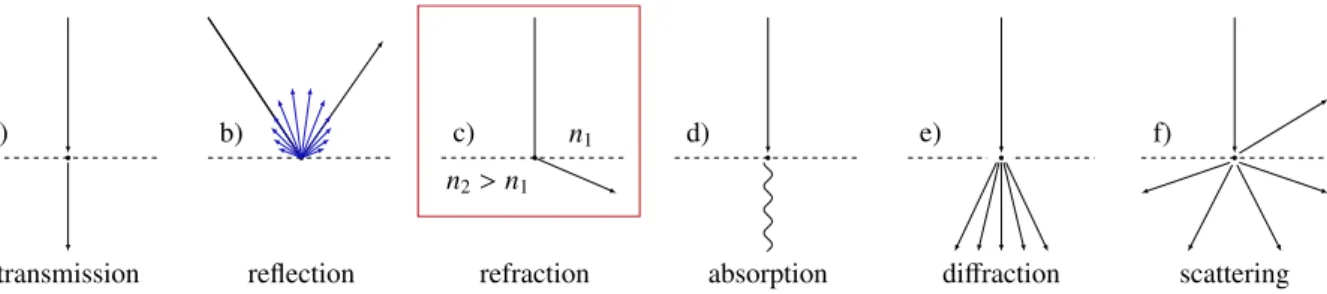
Figure 2.6 shows some of the possible interactions of a wave with the medium through which the wave is traveling. Besides others, the wave can be transmitted, reflected, refracted, absorbed, diffracted, or scattered.

a) b) c) d) e) f)

transmission reflection refraction

n2>n1 n1

absorption diffraction scattering

Figure 2.6:Wave behaviors: a) transmission; b) black: specular reflection, blue: diffuse reflection; c) refraction; d) absorption; e) diffraction; f) scattering. The red frame highlights the refraction causing the neutrospheric delays used in this work in order to reconstruct the 3D refractivity field.

If a wave is transmitted through the object, it can pass through the object without interacting with it. In the case of a specular reflection, the wave hits a smooth surface and bounces off. In this context, the signal’s wavelength must be large when compared with the roughness of the smooth surface. A wave (or a part of a wave’s energy) is absorbed if the wave causes a vibration of the atoms and molecules within the hit object. The vibration heats up the object and the heat is emitted as thermal energy. Diffraction corresponds to the bending of a wave when it encounters an obstacle. Scattering occurs when a wave encountering an object bounces off in many different directions.

Refraction occurs if a wave travels from a medium with some refractive indexn1to a medium with some other refractive indexn2resulting in a bending of the ray path as also observed in electronic distance measurements (EDM).

More information on refraction is given in Section 2.6, focusing particularly on ionospheric and neutrospheric refraction. The neutrospheric refraction is subdivided into refraction caused by the dry part of the neutrosphere and refractivity causing wet delays on radio wave signals. Thereafter, Section 2.6.1 explains how the dry delay can be modeled based on surface meteorological measurements, and the Sections 2.6.2 resp. 2.6.3 describe the effects of the wet refractivity on GNSS resp. InSAR observations and how information on the atmospheric water vapor can be deduced from these measurement techniques.

2.6 Path delay modeling in GNSS and InSAR

Both GNSS and InSAR satellites emit electromagnetic waves propagating, in vacuum, with the speed of lightc. On their way from the satellites to the ground (and back to the satellite, when thinking of InSAR), the signals pass the Earth’s atmosphere. Equation 2.16 describes the relation between the propagation velocityvin a medium with refractivityn:

n=c

v (2.16)

Fermat’s principle cited in Hofmann-Wellenhof et al. [2008] states that an electromagnetic signal follows the path between source and observer which takes the least amount of time. Due to the variation of the air masses or densities along the ray path of a radio wave, the refractive index nalong the signal transmitting path differs from that in vacuum and takes a value slightly greater than unity, varying along the signal’s path through the neutrosphere. As a consequence, according to Forssell [2008], the ray path deviates from a straight line and the signal propagation is delayed. The refractive index in Equation 2.16 is related to the total refractivity Ntotal by means of

Ntotal=106·(n−1). (2.17)

The ionospheric refraction is dispersive, i.e. depends on the signal’s frequency, whereas the neutrospheric refraction is related to the refractivity of gases, hydrometeors, and other particulates. The total refractivity and the total delay on radio wave signals caused by refractivity are commonly subdivided into two parts, e.g. into adryand awet

component or into a hydrostaticand anon-hydrostatic part. The following sections explain how to model the hydrostatic component of the delay by means of surface meteorology, and describe how to determine the wet component of the delay using GNSS Precise Point Positioning (PPP) resp. PS-InSAR.

2.6.1 Modeling the hydrostatic component of the delay using surface meteorology

As stated in Section 2.5, the total refractivity and the total delay on radio wave signals caused by refractivity are commonly subdivided into two parts, e.g. into adryand a wetcomponent or into ahydrostaticand a non-hydrostaticpart. According to Saastamoinen [1972], the hydrostatic component ZHD of the neutrospheric delay only contains the delay caused by dry gases and can be computed based on the surface pressurep0, the zenith angle

z, and correction termsDandBusing

ZHD=0.002277·D·h

p0−B·tan2zi. (2.18)

In contrast, when applying a subdivision into dry and wet components, the dry component ZDD=0.002277·D·h

also contains contributions of the partial pressure of water vapor at the surfacee0. In the Equations 2.18 and 2.19, the componentsDandBare correction terms, where Dis calculated from the ellipsoidal site heighth and the latitudeϕusing the formula

D=1+0.0026·cos2·ϕ+0.00028·hin km, (2.20)

andBis taken from lookup tables depending on the site heighth.

If a hydrostatic equilibrium can be assumed, the hydrostatic component can be accurately computed based on surface pressure. Therefore, in this work, the total refractivity or delay is subdivided into a hydrostatic and a non-hydrostatic part. However, for reasons of readability, and consistently with the International Earth Rotation and Reference Systems Service (IERS) conventions of Petit and Luzum [2010], the termswetrefractivity resp.

wetdelay are used in the following for the non-hydrostatic componentNwetof the refractivity resp. of the delay, yielding, with a hydrostatic refractivityNhydrostatic,

Ntotal=Nhydrostatic+Nwet (2.21)

resp.

ZTD=ZHD+ZWD. (2.22)

Figure 2.7 shows differences between dry and hydrostatic delays, which are based on surface meteorological observations in Karlsruhe. In humid summer months, the difference between Zenith Hydrostatic Delays (ZHD) and Zenith Dry Delays (ZDD) composing the Zenith Total Delays (ZTD) attains values of up to 4cm.

1 2 3 4 5 6 7 8 9 10 11 12 0.00 0.01 0.02 0.03 0.04 Month in 2005 ZHD -ZDD in m

Figure 2.7:Differences in m between dry and hydrostatic delays from surface meteorological measurements at Karlsruhe (synoptic site 4444).

As described in Section 2.6.3, a computation of the zenith hydrostatic delay is necessary both for deducing GNSS ZWDs and for deriving absolute ZWDs from a combination of partial InSAR ZWD differences, GNSS ZWDs, and surface meteorological observations. The ZHD is modeled using the Saastamoinen model from Equation 2.18. As surface meteorological measurements are often spatially poorly sampled, Dach et al. [2007] use standard at-mospheres in order to deduce the surface pressurep0, the surface temperatureT0, and the partial pressure of water vapor at the surfacee0 for the computation of the ZHD, see also Berg [1948]. Alternatively, the ZHD can be computed using surface meteorological observations. Based on pressure and temperature observationspmeteoand

Tmeteoof the closest synoptic site, Alshawaf et al. [2015b] and Alshawaf [2013] compute the pressurepGNSS at a certain location, e.g. a GNSS site, using the hydrostatic equation

pGNSS=pmeteo 1−LT·hGNSS_T −hmeteo meteo ! g·M_dryair R·LT (2.23) withhGNSSresp.hmeteostanding for the height of the considered GNSS site resp. for the height of the used surface meteorology site. The temperature lapse rateLT is equal to 6.5◦/km, the quantityg =9.80665m/s2is the mean

Earth’s gravity acceleration,Ris the universal gas constantR = 8.31447J/(mol·K), andMdryairis the molar mass of dry air. When applying Equation 2.23, in the case of a smooth topography, a meteorological site may be up to 100km distant to the GNSS site for which the pressure shall be computed.

If multiple meteorological sites are available close to the location for which the ZHD shall be computed, the pressure resp. temperature at the height of the location can be obtained by means of a linear regression model. To account for spatial variations, Alshawaf et al. [2015b] use the residuals of this linear regression to calculate a correction value at any point by applying, for example, inverse distance weighting.

2.6.2 Determining the wet component of the delay content using GNSS PPP

Subtracting the ZHD obtained from surface meteorological observations as described in the previous section from GNSS ZTDs yields the both spatially and temporally highly variable and thus difficult to precisely model neu-trospheric Zenith Wet Delay ZWD. The GNSS ZTDs are deduced from an overall least squares adjustment also yielding the receiver coordinates, the receiver clock correction, and the carrier-phase ambiguities.

In this work, the GNSS processing is performed using the PPP strategy introduced in 1997 by Zumberge et al. [1997]. In contrast to differential GNSS positioning approaches, PPP requires only one single receiver. As a refer-ence station is no longer necessary, the efforts and the equipment cost within the field work are reduced. Moreover, the PPP solution refers to a global reference frame whereas differential GNSS solutions are relative to the local base station. Therefore, PPP enables a greater positioning consistency than differential positioning. Moreover, there are no common parameters between the different sites to be solved within the PPP processing, which makes it possible to process the data site by site. Consequently, large networks can be processed on distributed systems using PPP. In return, the initialization time in PPP is longer than in differential positioning, which renders the use of PPP challenging in the case of real time measurements. Moreover, when compared to differential GNSS, orbit deviations and satellite clock offsets are no longer minimized or eliminated by building differences (Teunissen and Montenbruck [2017], Rizos et al. [2012]). That is, precise ephemerides as well as satellite clock corrections, provided e.g. by the International GNSS Service (IGS), are absolutely necessary in the case of PPP.

Since the satellite clock offset is known precisely for PPP, Kouba and Héroux [2001] describe the ionosphere-free linear combinationslρpseudo resp.lΦof dual-frequency GPS pseudo-range resp. carrier-phase observationsρpseudo andΦas a function of

• the geometric range between the satellite at its Earth Centered Earth Fixed (ECEF) coordinates (XSV,YSV,ZSV) and the receiver at its ECEF coordinates (xrec,yrec,zrec),

• the receiver clock offset∆t,

• the slant total delay STD obtained from the zenith total ZTD delay using STD=mf·ZTD with a mapping function mf,

• the ambiguityNof the carrier-phase at a carrier-phase wavelengthλΦ, • the constant speed of lightc,

• and measurement noise on the pseudo-range resp. on the carrier-phase signalρpseudo resp.Φ as shown in the following equation:

lρpseudo=ρgeom+c·∆t+mf·ZTD+ρpseudo

lΦ=ρgeom+c·∆t+mf·ZTD+N ·λΦ+Φ,

(2.24)

In Equation 2.24, the Euclidean distanceρgeombetween the satellite and the receiver is

ρgeom=

q

(XSV−xrec)2+(YSV−yrec)2+(ZSV−zrec)2. (2.25) By means of a linearization of the observation equation from Equation 2.24 around some a-priori parameters, a linear system of equations can be established that can then be solved using a least squares adjustment. The design