An analog hardware solution for compressive sensing reconstruction using gradient based method

R E S E A R C H

Open Access

An analog hardware solution for

compressive sensing reconstruction using

gradient-based method

Irena Orovi

ć

, Nedjeljko Leki

ć

, Marko Beko

and Srdjan Stankovi

ć

Abstract

This work proposes an analog implementation of gradient-based algorithm for compressive sensing signal reconstruction. Compressive sensing has appeared as a promising technique for efficient acquisition and reconstruction of sparse signals in many real-world applications. It starts from the assumption that sparse signals can be exactly reconstructed using far less samples than in standard signal processing. In this paper, we consider the gradient-based algorithm as the optimal choice that provides lower complexity and competitive accuracy compared with existing methods. Since the efficient hardware implementations of reconstruction algorithms are still an emerging topic, this work is focused on the design of hardware that will provide fast parallel algorithm execution for real-time applications, overcoming the limitations imposed by the large number of nested iterations during the signal reconstruction. The proposed implementation is simple and fast, executing 400 iterations in 1 ms which is sufficient to obtain highly accurate reconstruction results.

Keywords: Analog hardware, Compressive sensing, Gradient reconstruction method, Signal reconstruction

1 Introduction

In conventional digital signal processing, the sam-pling frequency needs to be at least the double of the maximal signal frequency in order to be able to get exact reconstruction of signals. Alternatively, in compressive sensing (CS) framework, the signal can be exactly recovered even when the number of avail-able samples is considerably below the conventional requirements [1–5]. Although certain conditions should be fulfilled for efficient CS scenario, it turns out that many signals in real applications are very conducive to CS. The first requirement is related to signal sparsity, which is generally achieved using certain transform domain representation [4–6]. The second one refers to incoherence between the

measurement process and the sparsity basis. In other words, a small set of linear measurements needs to be acquired in a random manner [4]. Under these conditions, the signal reconstruction is observed as a problem of solving undetermined system of linear equations. It is important to emphasize that the CS has been efficiently combined with different time-frequency approaches, either to define improved CS methods based on the time-frequency dictionaries or to define improved time-frequency representations based on the CS reconstruction principles [7]. A reliable instantaneous frequency estimation from a small set of available samples can be achieved by applying the signal reconstruction algorithms on the samples of the local autocorrelation function [8]. Therefore, the CS-based reconstruction methods bring several benefits to time-frequency analysis.

© The Author(s). 2019Open AccessThis article is distributed under the terms of the Creative Commons Attribution 4.0 International License (http://creativecommons.org/licenses/by/4.0/), which permits unrestricted use, distribution, and reproduction in any medium, provided you give appropriate credit to the original author(s) and the source, provide a link to the Creative Commons license, and indicate if changes were made.

* Correspondence:[email protected]

1_{Faculty of Electrical Engineering, University of Montenegro, Podgorica,}

Montenegro

Solving the problem of signal reconstruction from a small set of available samples can be a complex and demanding task from both software and hard-ware perspectives. The existing softhard-ware solutions [9–14] are mainly based on different iterative convex optimization techniques or their greedy iterative counterparts. These software implementations are generally unsuitable for real-time applications, due to the fact that the algorithms require a large num-ber of iterations to achieve convergence. Moreover, the intrinsic parallelism in the algorithm execution is difficult to achieve in a mono-processor computing system [15]. Therefore, in order to cope efficiently with signal reconstruction problem in compressive sensing, one needs a dedicated parallel hardware implementation of reconstruction algorithm. The hardware realization can be done using analog, digital, or combined analog and digital devices.

In this paper, we propose an analog hardware architecture of the gradient-based signal reconstruc-tion algorithm [14, 16]. The chosen algorithm ex-hibits optimal performance for different types of signals. It belongs to a group of convex optimization methods prominent for its accuracy and is computa-tionally less demanding than the other methods from this category. The proposed algorithm outperforms the standard ones used for the ℓ1-norm-based

minimization problems in both the calculation time and accuracy [16]. In huge contrast to greedy methods, the gradient-based algorithm does not re-quire the signal to be strictly sparse in a certain transform domain, rendering it suitable for real-world applications. Furthermore, it is well known the computational burden of digital hardware implemen-tation can be intensive, leading to long execution time [17–19]. Hence, opting for analog implementa-tion instead might bring considerable advantage in terms of complexity and consequently, to reduced execution time.

The paper is organized as follows. Theoretical

background on the compressive sensing and

gradient-based signal reconstruction algorithm is given in Section 2. Section 2 presents the proposed hardware solution, whose performance is discussed/ assessed in Section 3. The concluding remarks are given in Section 4.

2 Compressive sensing—theory and reconstruction method

Compressive sensing framework emerged from the efforts to decrease the amount of data sensed in the modern applications [5], and consequently to de-crease the needs for resources such as storage cap-acity, number of sensors, and consumption. The set

of measured data in traditional approach is usually referred to as full dataset, while the data in CS sce-narios are called incomplete dataset. The data sam-ples in the traditional sampling approach are equidistant and uniformly sampled, while in the CS, the data should be sampled randomly to achieve a high incoherence of the dataset. If the measurement process is modeled by a certain measurement matrix

Φ, then the measured dataset y of length M can be described as [2]:

y¼Φx ð1Þ

where x represents the full dataset of length N, and the measurement matrix is of size M × N, with M < < N. In practical scenarios, the CS dataset y and the measurement matrix Φ are known, and we de-sire to reconstruct the full dataset x of length N. However, the system of equations in (1) is underde-termined since M < < N. Thus, in order to tackle the problem, one resorts to the assumption that the signal x is sparse when represented in certain trans-form basis:

Χ¼Wx ð2Þ

where X is a transform domain representation of full signal dataset and W is the transform matrix, i.e.,

where Wi are the basis functions. Depending on

the signal, the basic functions could belong to discrete Fourier transform (DFT), discrete Hermite transform (DHT), discrete wavelet transform (DWT), discrete cosine transform (DCT), etc. For the sake of simplicity, we can write W as the coefficients’ matrix:

Sparsity means that the vector X has only K out of N nonzero (or significant) elements, while K < <

N and K < M. The system of linear equations becomes:

y¼ΦW−1_{X ð5Þ}

minimizek kX ₁ subject to y¼ΦW−1X ð6Þ

where ||X||1 denotes l1-norm. Generally, the l0

-norm is used to measure the signal sparsity, but in practical implementations, using the l0-norm can

lead to an NP problem; hence, the l1-norm is used

instead.

There are few types of algorithms that can be ap-plied for solving this problem and the most com-monly used are the convex optimization algorithms and the greedy algorithms [9, 10]. In general, the greedy solutions are simpler, but less reliable. Convex optimization algorithms are more reliable and accurate in general and guaranteed convergence, but their solutions comes at the cost of computa-tional complexity and large number of nested itera-tions [4, 9]. In this paper, we consider the gradient-based convex optimization algorithm as a representa-tive of the convex optimization group allowing sim-pler implementation compared with other common solutions.

2.1 Gradient-based signal reconstruction algorithm Assume that the missing samples positions are de-fined by the set Nm= {n1,n2, ...nN−M}. Now the

measurement vector is extended to the length of full dataset such that we embed zeros on the posi-tions of missing samples, i.e., y(n) = 0, forn∈Nm.

The gradient-based approach starts from some ini-tial values of unavailable samples (iniini-tial state) which are changed through the iterations in a way to constantly improve the concentration in sparsity domain. In general, it does not require the signal to be strictly sparse in certain transform domain, which is an advantage over other methods. In par-ticular, the missing samples in the signal domain can be considered as zero values. In each iteration, the missing samples are changed for +Δ and for

−Δ. Then, for both changes, the concentration is measured as l1-norm of the transform domain

vec-tors X+ (for +Δ change) and X− (for −Δ change), while the gradient is determined using their differ-ence. Finally, the gradient is used to update the values of missing samples. Here, it is important to note that each sample is observed separately and a single iteration is terminated when all samples are processed.

In the sequel, we provide a modified version of the algorithm adapted for an efficient hardware implementation avoiding complex functions and calculations.

The steps from the succeeding block are performed after the current block is processed. When the algorithm comes close to the minimum of the sparsity measure, the gradient changes direction for almost 180 degrees, meaning that the stepΔneeds to be decreased (line 18). The precision of the result in this iterative algorithm is estimated based on the change of the result in the last iteration.

3 Analog hardware implementation of modified gradient-based algorithm

From the modified version of the algorithm, we can identify following steps that need to be implemented within analog hardware architecture:

a) Set the signal samples at the input of analog architecture (line 0)

b) Set the digital signal identifying the positions of available and missing samples at the input of the architecture: positions of available samples are marked by value“1”(high voltage) and missing samples are marked by“0”(low voltage) values (line 0 in the modified algorithm).

c) Set the value for the gradient stepΔas in line 2 in the modified algorithm

d) Update the values of the gradientgfor input samples (lines 4 to 11 in the modified algorithm) e) Update the values of the missing samples andβ

(lines 12 and 13 in the modified algorithm) f) Check the condition for changingΔ(line 14 of the

modified algorithm):

– If the condition is not satisfied, repeat the steps d) and e) (lines 4 to 13 in the modified algorithm) Fig. 1The block scheme of the proposed analog architecture

Fig. 2Oscillator output signals (OSC_1,OSC_ 2,OSC_3, andOSC_4); T1, T2, T3, and T4 are durations of active states ofOSC_1,OSC_2,

– If the condition is satisfied,Δis decreased, for example, toΔ/3 (line 18 in the modified algorithm). It is noteworthy that in order to achieve high precision, the stepΔshould be decreased when approaching the stationary oscillations zone.

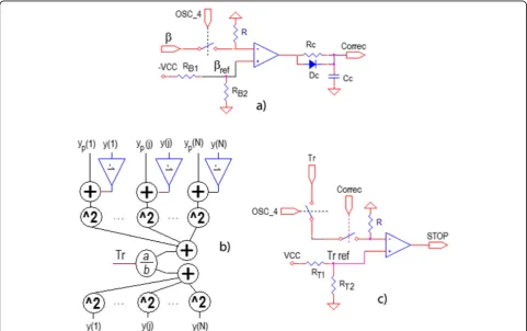
g) In parallel with changing the stepΔ, check the stopping criterion. The stopping criterionTris

defined as the mean value of changes applied on the missing samples using the previous value of

gradient stepΔ(line 19: in the modified algorithm). When the applied changes are less than the Fig. 3SetΔcorrection circuit

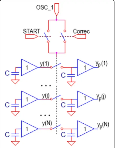
Fig. 4Block 1: sample and hold circuits controlled byOSC_1,START, andCorrecsignals used to updateyparray

predefined minimum, the updated value ofΔhas no significant influence on the signal quality and thus, the procedure should be stopped. In such a case, the current values of input signal represent the reconstruction result. If the stopping criterion is not met, the procedure is repeated with new updated valueΔ.

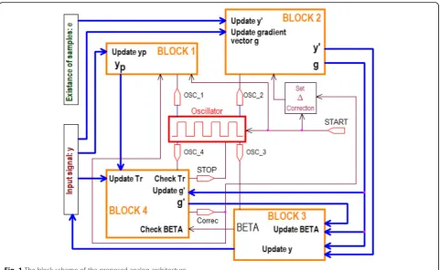
The block scheme for the proposed analog architec-ture is shown in Fig.1.

The architecture is composed of the following segments:

– Input array holding the analog samplesy,

– Input arrayeholding the indicators of available and missing samples positions,

– SetΔcorrection circuit,

– Four architecture blocks:Block1,Block2,Block3, andBlock4.

The proposed architecture blocks (Block 1, Block 2,

Block3, andBlock4) have been driven by the output sig-nals from the oscillator, namely OSC_1, OSC_2, OSC_3, andOSC_4, respectively. The sequence of active states of the oscillator’s signal controls the activation order of the four architecture blocks. Before theSTARTsignal, all out-puts are set to low voltage level. After activating START signal, the oscillator’s output signals are shown in Fig.2.

Prior to activating theSTART signal, the values of in-put signals y are loaded to the sample and hold ampli-fiers, and e values are set. During the START impulse, the initial value ofΔ is set to the output ofsetΔ

correc-tioncircuit, whose electrical diagram is shown in Fig.3. Let us briefly discuss the setΔcorrection circuit. By ac-tivating START signal, the capacitor C is loaded to the approximately maximal absolute value of the input sig-nal samples. It is the initial value of theΔcorrection.

Further update ofΔ is controlled by theCorrecsignal: when Correcis high, Δ is changed to Δ/3 (as in line 18 in the modified algorithm).

The architecture Block 1 is used to temporarily store values of y within the array yp(for the current value of Δ), Fig. 4.Block1 is active when OSC_1 (T1 impulse) is high and eitherSTART orCorrecsignal is active. At the beginning, during active state of START signal and first T1 impulse, the initial value of arrayy is loaded into the arrayyp. Further update ofypis controlled by active state

of OSC_1 signal and active state of the Correcsignal. It is important to note thatypvalues are updated each time

when a new correction valueΔ is set toΔ/3. Therefore,

yp represents the version of reconstructed signal at the

moment of applying a new Δ value. It is used later to calculate Tr (line 19 in the modified algorithm) as the

mean square error between y signal before and y signal after applying currentΔcorrection value.

The architecture Block 2 is active whenOSC_2 (T2 im-pulse) is high and it is used to update the values of the gradi-entsg(for each missing sample position), as shown in Fig.5. Current values ofyare placed iny′(for theith iterationy′=

y(i)

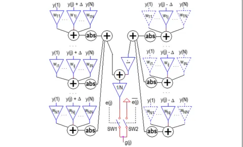
in the algorithm). The values of signal samples y are loaded into the sample and hold amplifiersy′. Further, the architectureBlock2 allows parallel computation of all gradi-ent samples ing. A circuit used to calculate a single gradient sample is shown in Fig.6. It consists of amplifiers represent-ing the transformation coefficientswijbelonging to the

trans-formation matrix W (defined in (5)), adders and absolute value circuits. The calculation of a gradient samplegirequires

N(N+ 1) + 1 amplifiers, 2(N+ 1) adders withNinputs, 2N absolute value circuits, 1 adder with two inputs, 1 invertor circuit, and 2 switches. Note that the amplifiers drawn by the dashed line (right side of Fig.6) are not supposed to be im-plemented in hardware. Namely, these amplifiers are shown in Fig.6only to provide a clearer circuit illustration, but the necessary values are already available at the output of the ap-propriate amplifiers on the left side of Fig.6. The switches in Fig.6are controlled by the signalecontaining the indicators of available and missing samples. The switchSW1 needs to be closed on the positions of missing samples and opened on the positions of available samples (the gradients are calcu-lated only for the missing samples positions), while the situ-ation with SW2 is opposite. Hence, at the position of available sample, the signale(i) keeps the switchSW1 open, while the signal eðiÞcloses theSW2 switch. At the position of missing sample, the signal e(i) keeps the switch SW1

closed, while the signaleðiÞopens the switchSW2. Fig. 8A circuits for updating parameterβ

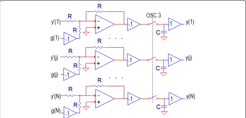
The architecture Block 3 is active when OSC_3 signal (T3 impulse) is high and it is used to obtain updated sig-nal valuesy using gradientgand current signal valuesy′ from Block 2 (y(i+1) = y(i) − g(i) in the algorithm). This part of Block 3 is shown in Fig. 7. Another part of the architecture Block3 is responsible for updating value of β(Fig.8). The value ofβis fed to the input of the circuit that validates the condition for changing the stepΔ.

The circuit in Fig. 8 consists of analog voltage adders, multipliers, squaring and rooting circuits, div-ision (multiplication) circuits, and sample and hold amplifiers. It can be seen that the calculation of β re-quires 3 adders with N inputs, N + 1 multiplier, 2N squaring circuits, two square-rooting circuit, and div-ision circuit. Note that the array denoted by g′ holds the gradient values from the previous iteration. Update of values ing′array is done inBlock4.

The architecture Block 4 is active when OSC_4 sig-nal (T4 impulse) is high and it is used to load current values from g into g′. The circuits in Block 4 are fur-ther used to check the parameterβand activateCorrec signal (Fig. 9a), update the value of Tr (Fig. 9b), and

check whether the stopping criterion is met (Fig. 9c). The circuit in Fig. 9b consists of the adders (N + 2), multipliers, N inverters, 2N squaring analog voltage

circuits, and 1 division circuit. The circuit in Fig. 9 a comparesβandβREF, and ifβ<βREF, the signal Correc

is activated as a trigger to update the value of Δ. The active state of signal Correc allows us to check the stopping criterion (Fig.9c). If the stopping criterion is met, the STOP signal is activated. This causes deacti-vation of all oscillator outputs and consequently all switches in the hardware become open. In the case where the stopping criterion is not met, RcCc time constant is used to keep the high voltage ofCorrec sig-nal for the next T1 period. It is used to enable update of sample and hold amplifiers denoted byyp.

The required components per block are shown in Table 1 (only the main and most represented compo-nents are listed, such as amplifiers, adders, and multipliers).

4 Results and discussion

The simulation of the proposed hardware architec-ture is done using the PSpice (OrCAD 16.6). For the realization of multipliers, division circuit, squaring, and square-rooting circuit the analog device AD734 is used. The circuit represents a precise four-quadrant high-speed analog multiplier that is able to perform all the abovementioned functions. For the

Fig. 9Circuits in block 4:achecking the conditionβ<βREF(if the condition is satisfied,Correcsignal is activated),bupdating the threshold value

realization of amplifiers (inverters), adders and abso-lute value circuits, we employed the ultra-high-speed operational amplifier LT1191. For the analog voltage comparison, we employed the circuit LT1394 (com-parator) [20] (with settling time 7 ns). The circuit provides the complementary outputs and allows the zero-crossing detection. The sample and hold cir-cuits AD783 are used for storing the voltage values. Furthermore, in the simulation, we used the analog switches MAX4645 [21] and diodes 1 N4448 [22].

The simulation has shown that the required duration for the oscillator outputs are T1 ≈ 320 ns, T2 ≈ 740 ns, T3 ≈ 650 ns, and T4≈ 610 ns. The time between the impulses (Tp) is required to turn off the analog switches used in the proposed hardware. The turn off time for switches MAX4645 is up to Tp = 40 ns. Hence, the minimal duration for one algorithm iteration is T1 + T2 + T3 + T4 + 4Tp = 2.48μs ≈ 2.5μs. The total calculation time for the reconstruc-tion of an input signal depends on the number of iter-ations. The proposed solution allows up to 400 iterations within 1 ms, and it is interesting to mention

that most of the signals in real applications can be completely accurately reconstructed within a few hun-dreds of iterations [16].

Another advantage of the proposed hardware solution is the robustness on hardware imperfection. The used components generate a very small error. The main source of errors is the circuit AD734. However, it con-tributes in error with typical 0.1% of the full scale or 0.25 in full temperature range from–40 to + 85 °C. Our simulations have shown that the maximal introduced error can cause only a few additional iterations to achieve a high precision reconstruction performance, which is negligible in terms of time and processing costs.

4.1 Example

In order to provide an illustration of signal reconstruc-tion results, let us observe the experimental synthetic signal that is sparse in the Hermite transform domain. The original signal contains 64 samples, but only 26 samples are available on the random positions within the signal, while 38 samples are missing and should be

Table 1The number of the most represented circuits required

Input signal circuits Block1 Block2 Block3 Block4 Total

Amplifiers N3+N2+ 3N 2N N N3+N2+ 6N

Adders 2N2+ 4N N+ 3 N+ 2 2N2+ 6N+ 5

Absolute value circuits 2N2 2N2

Sample and hold amplifiers N N 2N 1 N 5N+ 1

Switches N+ 2 4N N+ 1 N+ 3 7N+ 6

Multipliers/divisions 3N+ 4 2N+ 1 5N+ 5

reconstructed. The available samples are shown in Fig.10a. The original signal with missing samples marked in red color is shown in Fig.10b. The reconstructed signal is shown in Fig. 10c. The sparse Hermite transform after the reconstruction is shown in Fig. 10d. The achieved mean square error is of order 10−3 which can be con-sidered negligible in the case of observed signal. Thus, the reconstruction result is highly accurate.

In real-world applications, the same concept can be applied for the reconstruction of QRS complexes (as shown in Fig. 11) in ECG signals, or ultra-wide band (UWB) signals in communications, that are also sparse in the Hermite transform basis. In the case of other communications signals (e.g., FHDSS), the Fourier trans-form basis would be more appropriate for achieving sparse signal representation. Finally, without loss of gen-erality, this approach can be applied in the same way by using any other transform basis as long as it allows sparse representation of the specific observed signal. Therefore, the proposed hardware implementation is very amenable to various practical applications, for in-stance in communications, radars and remote sensing, biomedicine, etc.

5 Conclusion

In this work, we presented an analog hardware archi-tecture for gradient-based algorithm for sparse signal reconstruction. The algorithm is suitable for different types of signals and therefore is suitable for real-time implementation which opens a wide range of applica-tions, including time-frequency signal analysis and instantaneous frequency estimation. The proposed

analog design allows fast processing and low-complexity realization, executing significant number of algorithm iterations in short-time intervals (at the order of 1 ms), which is highly satisfactory for real-time applications.

Abbreviations

CS:Compressive sensing; DFT: Discrete Fourier transform; DHT: Discrete Hermite transform; DWT: Discrete wavelet transform; DCT: Discrete cosine transform

Acknowledgements Not applicable.

Authors_’contributions

All authors made contributions in the discussions, analyses, and

implementation of the proposed hardware solution. IO and NL were actively involved in writing the manuscript. All authors read and approved the final manuscript.

Funding

There are no financial sources of funding for the research to be reported.

Availability of data and materials

Data sharing not applicable to this article as no datasets were generated or analyzed during the current study.

Consent for publication

The manuscript does not contain any individual person’s data in any form (including individual details, images, or videos) and therefore the consent to publish is not applicable to this article.

Competing interests

The authors declare that they have no competing interests.

Author details

1_{Faculty of Electrical Engineering, University of Montenegro, Podgorica,}

Montenegro.2_{COPELABS, Universidade Lusófona de Humanidades e}

Tecnologias, Lisbon, Portugal.

Received: 20 August 2019 Accepted: 22 November 2019

References

1. D. Donoho, Compressed sensing. IEEE Trans. Inf. Theory52(4), 1289–1306 (2006)

2. R. Baraniuk, Compressive sensing. IEEE Sig. Proc. Magazine.24(4), 118–121 (2007) 3. M. Elad, Sparse and redundant representations: from theory to applications

in signal and image processing. Springer (2010)

4. S. Foucart,H Rauhut, A mathematical introduction to compressive sensing

(Springer, New York, 2013)

5. S. Stankovic, I. Orovic, E. Sejdic,Multimedia signals and systems: basic and advance algorithms for signal processing, 2nd edn. (Springer-Verlag, New York, 2015)

6. Y.C. Eldar,Sampling theory: beyond bandlimited systems, (Cambridge University Press)(2015)

7. E. Sejdić, I. Orović, S. Stanković, Compressive sensing meets time-frequency: an overview of recent advances in time-frequency processing of sparse signals. Digital Signal Processing77, 22–35 (2018)

8. I. Orović, S. Stanković, T. Thayaparan, Time-frequency based instantaneous frequency estimation of sparse signals from an incomplete set of samples. IET Signal Processing8(3), 239_–245 (2014)

9. E. Candes, T. Tao, Decoding by linear programming. IEEE Trans. Inf. Theory 51(12), 4203–4215 (2005)

10. J. Tropp, A. Gilbert, Signal recovery from random measurements via orthogonal matching pursuit. IEEE Trans. Inf. Theory53(12), 4655_–4666 (2007) 11. A. Draganić, I. Orović, and S. Stanković,“On some common compressive

sensing recovery algorithms and applications—review paper,”Facta Universitatis, Series: Electronics and Energetics, Vol 30, No 4 (2017), pp. 477-510, DOI Number 10.2298/FUEE1704477D, December 2017

12. J. Music, I. Orovic, T. Marasovic, V. Papic, S. Stankovic, Gradient compressive sensing for image data reduction in UAV based search and rescue in the wild, Mathematical Problems in Engineering, 2016 (ID 6827414), 14 pages 13. N. Leki_ć, A. Dragani_ć, I. Orovi_ć, S. Stankovi_ć, and V. Papi_ć,_“Iris print extracting

from reduced and scrambled set of pixels,”Second International Balkan Conference on Communications and Networking BalkanCom 2018, Podgorica, Montenegro, June 6-8, 2018

14. M. Brajovic, I. Orovic, M. Dakovic, S. Stankovic, Gradient-based signal reconstruction algorithm in the Hermite transform domain. Electron. Lett 52(1), 41–43 (2016)

15. N. Nedjah, R. M. da Silva, L. de Macedo Mourelle, Analog hardware implementation of artificial neural networks, J. of Circuit Syst. and Comp., 20(3), 349-373 (2011).

16. L. Stankovic, M. Dakovic, On a gradient-based algorithm for sparse signal reconstruction in the signal/measurements domain, Mathematical Problems in Engineering, 2016 (ID 6212674), 11 pages.

17. S. Vujovic, M. Dakovic, I. Orovic, S. Stankovic, An architecture for hardware realization of compressive sensing gradient algorithm, in Proc. 4th Mediterranean Conference on Embedded Computing, MECO 2015, Budva, Montenegro, 2015.

18. I. Orović, A. Draganić, N. Lekić, and S. Stanković,“A system for compressive sensing signal reconstruction,”17th IEEE International Conference on Smart Technologies, IEEE EUROCON 2017

19. N. Zaric, N. Lekic, S. Stankovic,_“An implementation of the L-estimate distributions for analysis of signals in heavy-tailed noise,”IEEE Transactions on Circuits and Systems II, Vol 58. No.7, pp. 427-432, 2011

20. LINEAR TECHNOLOGY CORPORATION, 7 ns, Low Power, Comparator– LT1394 (datasheet). 16 pages, [Online]. Available at:http://cds.linear.com/ docs/en/datasheet/1394f.pdf. Accessed Apr 2019.

21. MAXIM, Fast, Low-Voltage, 2.5Ω, SPST, CMOS Analog Switches–MAX4645 (datasheet). 11 pages, [Online]. Available at:https://datasheets.

maximintegrated.com/en/ds/MAX4645-MAX4646.pdf. Accessed Apr 2019. 22. VISHAY SEMICONDUCTORS, Small Signal Fast Switching Diodes–1 N4448 (datasheet). 4 pages, [Online]. Available at:http://www.vishay.com/docs/81 858/1n4448.pdf. Accessed Apr 2019.

Publisher’s Note