University of South Carolina
Scholar Commons
Theses and Dissertations
1-1-2013
Essays On Market Dominance and Price Discovery
James Michael Lockwood University of South Carolina - Columbia
Follow this and additional works at:https://scholarcommons.sc.edu/etd
Part of theBusiness Administration, Management, and Operations Commons
This Open Access Dissertation is brought to you by Scholar Commons. It has been accepted for inclusion in Theses and Dissertations by an authorized administrator of Scholar Commons. For more information, please [email protected].
Recommended Citation
E
SSAYS ONM
ARKETD
OMINANCE ANDP
RICED
ISCOVERYby
James M. Lockwood
Bachelor of Science
David Lipscomb University, 2004
Submitted in Partial Fulfillment of the Requirements
For the Degree of Doctor of Philosophy in
Business Administration
The Darla Moore School of Business
University of South Carolina
2013
Accepted by:
Eric A. Powers, Major Professor
Timothy W. Koch, Committee Member
Steven V. Mann, Committee Member
Peter R. Locke, Committee Member
ii
© Copyright by James M. Lockwood, 2013
iii
ACKNOWLEDGMENTS
I gratefully acknowledge the support, encouragement, patience, and advice offered by my
dissertation committee members, Professors Timothy Koch, Steven Mann, and Peter
Locke. I also thank Professors Tom McInish of the University of Memphis, Sanjiv
Sabherwal of the University of Texas, P. K. Jain of the University of Memphis, and
Martin Herrera of Monterey Tech University, and to participants at the speaker series at
the University of Memphis, Texas Christian University, the University of Texas, and
Colorado State University for their many helpful comments on previous drafts of this
dissertation. I am indebted to Professor Sie Ting Lau of the Nanyang Technical
University in Singapore for providing access to the Securities Industry Research Centre
of Asia-Pacific (SIRCA) database. I especially thank and acknowledge the guidance,
encouragement, patience, and wisdom so generously offered to me by my dissertation
iv ABSTRACT
In the first essay, I examine the burden of cross-listing prices to adjust to changes in
exchange rates. Using a 3-system vector moving average model, I measure the effects of
exchange rate shocks on cross-listing stock prices in the home and U.S. markets. My
sample consists of 46 cross-listings on the NYSE from Canada, Brazil, and Mexico.
Findings indicate that New York prices bear roughly 60% of the adjustment to exchange
rates for Canadian and Mexican securities, and roughly 45% for Brazilian securities. The
NYSE burden of adjustment varies considerably across firms, ranging from 7% to 100%
for Canada, 10% to 79% for Brazil, and 24% to 90% for Mexico. Tests show that the
NYSE burden to adjust to exchange rate changes is highest for big firms, and for those
with relatively high NYSE trading costs or low NYSE trading volume. For the majority
of firms, tests also show that the combined markets burdens to adjust to exchange rates
increase during the period of heightened exchange rate volatility. My results have
important implications for international price discovery tests, especially for those that fail
to model an independent role for exchange rates at the firm level.
In the second essay, I examine the dynamics of price discovery for markets with
varying market characteristics. I estimate Hasbrouck’s (1995) information share over two
distinct time periods of 2008 for my sample of 23 Canadian firms, 13 Brazilian firms, and
10 Mexican firms. In contrast to most prior research, I find that the home market does not
v
discovery leader. Findings show that the price discovery on the NYSE is higher for
cross-listings with greater NYSE market depth, lower burden to adjust to exchange rates on the
NYSE, with greater trading volume and lower cost, and for smaller, low market-to-book
firms. Findings show that market depth and the burden of prices to adjust to exchange
rate shocks are key determinants for price discovery that rival the importance of trading
volume and cost.
vi
TABLE OF CONTENTS
ACKNOWLEDGEMENTS ... iii
ABSTRACT ... iv
LIST OF TABLES ... vii
LIST OF FIGURES ... viii
CHAPTER 1LOST IN TRANSLATION ...1
1.1 METHODOLOGY ...5
1.2 DATA ...9
1.3 TESTABLE PROPOSITIONS ...11
1.4 RESULTS ...11
1.5 CONCLUSIONS ...23
CHAPTER 2MARKET DOMINANCE AND PRICE DISCOVERY ...40
2.1 RELATED CROSS-LISTING AND EQUITY PRICE DISCOVERY LITERATURE ...42
2.2 STOCK TRADING DETAILS FOR CANADA,BRAZIL, AND MEXICO ...47
2.3 THE DATA AND METHODOLOGY ...52
2.4 TESTABLE PROPOSITIONS ...64
2.5 RESULTS ...67
2.6 SUMMARY AND CONCLUSIONS...78
REFERENCES ...95
vii LIST OF TABLES
TABLE 1.1CANADIAN SAMPLE SUMMARY ...25
TABLE 1.2BRAZILIAN SAMPLE SUMMARY ...26
TABLE 1.3MEXICAN SAMPLE SUMMARY ...27
TABLE 1.4EXCHANGE RATE EFFECTS FOR THE CANADIAN SAMPLE ...28
TABLE 1.5EXCHANGE RATE EFFECTS FOR THE BRAZILIAN SAMPLE ...29
TABLE 1.6EXCHANGE RATE EFFECTS FOR THE MEXICAN SAMPLE ...30
TABLE 1.7SUMMARY STATISTICS FOR THE NYSETRANSLATION RISK PERCENTAGE ...31
TABLE 1.8TRPQUINTILE SUMMARY STATISTICS ...32
TABLE 1.9TRPREGRESSIONS ...33
TABLE 2.1CANADIAN CROSS-LISTING SAMPLE ...81
TABLE 2.2BRAZILIAN ADRSAMPLE ...82
TABLE 2.3MEXICAN ADRSAMPLE ...83
TABLE 2.4DESCRIPTIVE STATISTICS ...84
TABLE 2.5MARKET CHARACTERISTICS PERCENTAGE DOMINANCE ...86
TABLE 2.6CROSS-SECTIONAL PRICE DISCOVERY TESTS,PRE-CRISIS PERIOD ...87
TABLE 2.7CROSS-SECTIONAL PRICE DISCOVERY TESTS,CRISIS PERIOD ...88
viii LIST OF FIGURES
FIGURE 1.1EXCHANGE RATES ...34
FIGURE 1.2IMPULSE RESPONSE FUNCTIONS ...36
FIGURE 1.3PLOT OFˆHOME E, VERSUS ˆNYSE E, ...37
FIGURE 1.4COMBINED MARKETS BURDEN TO ADJUST TO EXCHANGE RATES ...39
FIGURE 2.1THE VIXINDEX 2008 ...90
1
CHAPTER 1
LOST IN TRANSLATION:
WHICH STOCKS BEAR THE BURDEN TO ADJUST TO EXCHANGE RATES
?
The efficient markets hypothesis assumes that security market prices rapidly reflect new
information, making it very difficult to “beat the market.” However, the efficient markets
hypothesis is agnostic regarding precisely where new information is first reflected for
securities that trade in more than one marketplace, i.e. where price discovery occurs.
Recent research attempts to locate where price discovery occurs for stocks that cross-list
internationally, but often ignores the informational role of exchange rates in the price
formation process.1 In related work, Grammig et al. (2005) offer simulations showing that the failure to properly model exchange rates leads to biased price discovery
estimates, especially during periods of high exchange rate volatility.
The goal of my study is to measure the effect of exchange rate shocks on stock
prices for cross-listings from distinct markets over volatile currency time periods. My
study is designed to provide robust tests of the independent informational role of
exchange rates in the price discovery process. Specifically, I assess the impact of
exchange rate shocks on U.S. and home market prices for 46 cross-listings on the NYSE
from Canada, Brazil, and Mexico during 2008, one of the most volatile periods for stocks
1 Most firms list in the U.S. via ADRs, which originate from many countries. In contrast, direct
2
and currencies in recent history. The three home markets are characterized with different
degrees of financial development, investor protection, insider trading law enforcement,
liquidity, cost, and trading volume. Also, the markets provide the largest number of
cross-listings, and the three markets span the continuum from developed market (Canada)
to emerging market (Mexico). While the three markets share significant intraday trading
overlap, the geographic proximities of each market to New York differ substantially. All
three markets are major economic trade partners with the U.S. For instance, as of 2010,
U.S. is the top economic trade partner with Canada and Mexico and is the second biggest
trade partner with Brazil, all of which suggests that the markets might share in the burden
to adjust to exchange rates more equally versus the three German stocks studied by
Grammig et al. (2005).
Most cross-listing price discovery papers examine relations between home prices
and foreign prices, after converting prices to a common currency. Each cross-listing into
the U.S. signifies ownership in the underlying security originating from the foreign
market. In the absence of arbitrage restrictions, the law of one price suggests that the two
securities be priced identically, at all points in time, after adjusting for exchange rates.
However, exchange rate shocks might exert an independent effect on stock prices, and
the effect may be asymmetric for the home and foreign markets. For example,
depreciation of the Mexican peso versus the U.S. dollar (alternatively, appreciation of the
dollar versus the peso) likely will lead to an increase in the peso price of the security on
the BOLSA and a decrease in the dollar price on the NYSE. But, no evidence exists to
suggest that the two prices will automatically meet in the middle. Nor is there evidence
3
implicitly made by most cross-listing studies when converting prices to a common
currency.
Grammig et al. (2005) show that the choice of currency conversion matters. Their
simulation shows that price discovery inferences depend on whether the home currency is
converted to the foreign currency or if the foreign currency is converted to the home
currency, and that the errors in inference increase with the volatility of exchange rates.
The authors also examine three German stocks that cross-listed between the Frankfurt
and New York Stock Exchange during the three month period August 1999 – October
1999. Relying on tests that endogenize the exchange rate, their findings show that most of
the exchange rate burden was borne by the NYSE. The authors conclude that the foreign
investor “is subject to exchange rate risk in that prices incorporate another source of
uncertainty beyond the value of the firm itself, and this is not the case for the
home-market investor.”
The Grammig et al. (2005) paper makes important contributions, but is limited
with respect to the number of stocks, concentration of stocks in a dominant home market,
short overlapping intraday trading interval, and examination of relatively stable dollar to
euro exchange rates. Whether exchange rate uncertainty truly imposes a burden on
foreign investors and whether this relationship holds outside the Germany-U.S. country
3-stock pairing is unknown. In contrast, my tests are conducted on a sample characterized
by a greater mix of “international” and domestic firms versus the three blue chip German
stock sample studied by Grammig et al. (2005), and span a period of significant stock
4
To estimate the burden borne by each stock to adjust to exchange rate shocks, I
develop a 3-system vector moving average model that produces impulse response
coefficients related to exchange rate shocks. I create a translation risk measure equal to
the percentage of the exchange rate – stock price adjustment borne by the NYSE relative
to the combined adjustments of the NYSE and home markets. A high (low) percentage
indicates that the NYSE (home) bears most of the burden to adjust to exchange rate
shocks.
My tests show that New York prices bear roughly 60% of the adjustment to
exchange rates for Canadian and Mexican securities, and roughly 45% for Brazilian
securities. Results differ markedly across firms and across time, and show that the
combined markets’ burdens to adjust to exchange rates increase during the period of high
exchange rate volatility. Therefore, the burden of prices to adjust to exchange rate shocks
is not homogeneous within country, and is sensitive to exchange rate volatility. I find that
the burden on New York prices to adjust to exchange rates is higher for larger firms and
for firms with lower trading volume and higher bid-ask spreads on the NYSE versus the
home market. These findings indicate that the burden of prices to adjust to exchange rates
is expected to shift more to emerging markets as the migration of cross-listing trading
volume to the NYSE increases.
My study has important implications for price discovery tests that ignore the
informational role that exchange rates have on stock prices. Tests that fail to model the
independent effect of exchange rates produce misleading price discovery results. In
particular, these tests measure the combined effect on prices of fundamental news about
5
In my tests, I am able to disentangle the effects on stock prices of firm-specific
fundamental news and exchange rate news. Also, I am able to show the extent to which
each stock’s price discovery is affected by the exchange rate burden. My findings show
that the exchange rate burden is not a broad market-based effect, but instead is a
stock-specific effect. Therefore, any attempts to model the effect of exchange rates with
market-wide adjustments are wrong.
The plan of the paper is as follows. The methodology is explained in Section 1.
The data are detailed in Section 2. Testable propositions are presented in Section 3.
Results are discussed in Section 4, and concluding remarks are offered in Section 5.
1.1. Methodology
For any cross-listing, log prices are assumed to evolve by the following processes:
, ,
HOME t t HOME t
P P (1.1)
, ,
NYSE t t NYSE t
P P (1.2)
1 ,
t t P t
P P (1.3)
/ , / , 1 ,
H US t H US t E t
E E (1.4)
Ptis the equilibrium (log) price stated in the home currency, and EH/USis the
log-transformed home price of one US dollar. By assumption, the innovations
,, ,, ,,
HOME t NYSE t P t
and E t, are serially and contemporaneously uncorrelated with zero
mean.
Ignoring microstructure issues such as trading frictions and costs for the moment,
the home price must equal the currency converted NYSE price, using the law of one price
6
rate equals the NYSE price converted to the home currency. The natural log of the
product of the prices equals the sum of the natural logs: PNYSE t, EH US t/ , . Thus, in order
for the law of one price to hold in the 3-system model, PHOME t, PNYSE t, EH US t/ ,.2 With
this set-up, the 3-system error correction model can be expressed as:
, , 1 , 1 / , 1 , , ,
1
, , , , , / , ,
1 1
( )
N
HOME t HOME HOME HOME t NYSE t H US t HOME HOME i HOME t i
i
N N
HOME NYSE i NYSE t i HOME E i H US t i HOME t
i i
P c P P E P
P E
(1.5), , 1 , 1 / , 1 , , ,
1
, , , , , / , ,
1 1
( )
N
NYSE t NYSE NYSE HOME t NYSE t H US t NYSE HOME i HOME t i
i
N N
NYSE NYSE i NYSE t i NYSE E i H US t i NYSE t
i i
P c P P E P
P E
(1.6)/ , , 1 , 1 / , 1 , , ,
1
, , , , , / , ,
1 1
( )
N
H US t E E HOME t NYSE t H US t E HOME i HOME t i
i
N N
E NYSE i NYSE t i E E i H US t i E t
i i
E c P P E P
P E
(1.7)The equations indicate that prices respond to the prior period’s deviation from the
long-run equilibrium (the error correction term), and to lagged changes in prices and exchange
rates.
Equations 1.5 – 1.7 can be restated in matrix form, as
1 1
' ,
N
t t i t i t
i
p c p p
(1.8)
2 Stated differently, the log home price minus the sum of the log NYSE price and the log exchange rate
equals HOME t, (NYSE t, EH US t/ , ),where HOME t, NYSE t, EH US t/ , is the exchange rate adjusted log pricing error on the NYSE. Therefore, the linear combination of the log price on the home market, the log price on the NYSE, and the log exchange rate equals the difference in the currency-adjusted pricing errors
, ( , / , ).
HOME t NYSE t EH US t
This result implies that the linear combination of the log prices and exchange rate is stationary, and that the log home price, log NYSE price, and log exchange rate are cointegrated with cointegrating vector (1, 1, 1);e.g, (1, -1, -1)×(PHOME, PNYSE, EH/US)′ = PHOME – (PNYSE + EH/US) =
, ( , / , ).
HOME t NYSE t EH US t
7
where, ∆pt is the 3 × 1 vector of changes in prices (∆PHOME,t , ∆PHOME,t, ∆EH/US,t )′, c is 3 ×
1 vector of constants, α is the 3 × 1 vector of adjustment parameters, β′ is the 1 × 3
cointegrating vector, pt-1 is a 3 × 1 vector of prices for period t-1, iare 3 × 3 matrices of
autoregressive coefficients for lag i = 1, 2, …, N, and εt is the 3 × 1 vector of error terms.
If the law of one price holds in the long run, then prices are cointegrated, and β′ = (1 1,
-1).
Employing the Wold Representation Theorem on Equation (1.8) yields:
1 1 2 2 ( )
t t t t t
p L
(1.9)
where each i is a 3 × 3 vector moving average (VMA) matrix. Next, the Beveridge and
Nelson (1981) decomposition is applied to( )L
t, and summing over time to yield:* 0
1
(1) ( )
t
t s t
s
p p L
(1.10)where (1) I
1 2 , and measures the long-run impact of a shock to the level of prices, and Ψ* is a matrix polynomial. Estimating the(1) matrix is the cornerstone ofthe analysis since the elements contain information about the permanent effect that each
of the innovations exert on the long-run dynamics of the prices. The values of the (1)
elements can be backed out of the parameterized VEC model Equation (1.8) by
computing the impulse response functions.
To derive the permanent impacts associated with price innovations, I apply Stock
and Watson’s (1988) common trends representation for cointegrated systems, in which:
, , , , , , , , , , , , (1) HOME t
HOME HOME HOME NYSE HOME E
t NYSE HOME NYSE NYSE NYSE E NYSE t
E HOME E NYSE E E E t
8
Each ijrepresents the permanent impact on price i of an innovation in price j. For example, HOME NYSE, is the long-run impact on the home market price of a shock to the
NYSE price, HOME E, is the long-run impact of a shock to the home market price of a shock to the exchange rate, etc. Given that the elements in the vector pt are ordered as
,, ,,
HOME t NYSE t
P P and EH US/ , the first row of (1)
t,, , , , , ,
HOME HOME HOME t HOME NYSE NYSE t HOME E E t
, gives the long-run component of the
innovations that are permanently impounded in the home market price.
The coefficients HOME E, and NYSE E, measure the long-run impacts of a shock to
the exchange rate on prices on the home market and the NYSE, respectively. These
coefficients are particularly important because they capture any asymmetric responses of
stock prices to changes in exchange rates, and are used to measure the NYSE burden to
adjust to exchange rates (or TRP).
For each stock, I create a translation risk percentage (TRP) equal to:
, , , ˆ ( ) ˆ (ˆ ) NYSE E
HOME E NYSE E
ABS TRP ABS
(1.12)
Either PHOME t, must respond (as measured by HOME E, ) to the exchange rate shock, or
,
NYSE t
P must respond (as measured by NYSE E, ) to the exchange rate shock, or both series
must respond.The sum of both parameters (in absolute value) can be interpreted as the
combined total response to an exchange rate shock. If responses to an exchange rate
shock are symmetric then TRP will equal 0.5. On the other hand, a high TRP indicates
9
To date, no study focuses explicitly on the identification of markets that bear the
brunt of the exchange rate burden across a diverse set of firms. There is no reason to
expect that markets will respond symmetrically to exchange rate shocks such that TRP
equals 50%. Robust tests of exchange rate effects are offered in the current study that
examines a diverse sample in terms of individual companies, industry affiliations, and
countries, as well as a more volatile currency time period and intraday trading overlaps.3
1.2. Data
I use tick-by-tick quote and price data from the Securities Industry Research Centre of
Asia-Pacific (SIRCA) database, which is the standard source for international intraday
data. SIRCA receives the original data from Thomson-Reuters, and provides global
intraday trade, quote, and market depth for stocks and other instruments.4 Data used in the cross-sectional tests are derived from Datastream, Bloomberg, and SEC filings. My
sample includes 10 Mexican, 13 Brazilian, and 23 Canadian cross-listings for 2008. I
adjust U.S. prices for changes in the exchange rate using intraday bid and ask exchange
rate quotes obtained from Olsen and Associates. The following steps summarize my data
collection and management procedures.
Starting with the raw tick-by-tick quote data, I create 1-minute interval data
points. I drop observations with a spread equal to or less than 0, then capture the closing
bid/ask quote for each minute and assign it to that minute-interval. Obvious data errors
3 Although not focused on the identification of markets that bear the brunt of the exchange rate burden,
Grammig et al. (2005) conduct tests on three German stocks that cross-list onto the NYSE and find that New York prices respond more than Frankfurt prices to exchange rates. Their result is not surprising in light of their limited sample from a dominant home market. The main purpose of their study is offer simulations of the effects of endogenizing exchange rates, not on empirical tests of exchange rate burdens. For example, their empirical data are characterized by brief intraday trading overlaps (25% of the trading day), limited sample size, and stable exchange rates.
4 Thomson Reuters Tick History provides millisecond time-stamped data for over 35 million OTC
10
(negative spreads, zero spreads, or outrageous spreads) are eliminated.5 In my final screen for errors, I filter the data using the Billor et al. (2000) blocked adaptive
computationally efficient outlier nominators (BACON) method. The BACON approach is
computationally efficient, and is particularly appropriate for large datasets. The BACON
method begins by identifying a subset of the sample (called the “basic sample”) that is
“safely” free of outliers. Then, the method iteratively expands on the basic sample by
creating a new basic sample containing observations with acceptable Mahalonobis
distances relative to the previous basic sample median (or mean). The acceptable distance
is chosen using a percentile of the chi-square distribution. Billor et al. used the 95th percentile in their simulation. The iterations continue until the size of the basic sample
stabilizes. I replace all outliers with quote data from the previous minute. As explained by
Hasbrouck (2007), unlike transactions data, quote-midpoints can be propagated forward
because bid-ask quotes are considered open until a change is reported.
To avoid the disproportionate loss of observations clustered around significant
volatility events, I applied the procedures in a univariate manner to each stock separately
for each day. I also visually inspected every stock in the sample for data errors by
graphing prices and exchange rates at 1-minute intervals. The procedures did very well
identifying outliers without loss of information. Note that it is common to filter
microstructure data, as pointed out in many microstructure papers (see, for example,
Kryzanoski and Zhang (2002) and Brennan and Subrahmanyam (1996)).6
5 I define an outrageous spread as greater than 70% of the quote midpoint. Garfinkel (2009), Chung and
Zhang (2009) delete observations where the bid-ask spread is greater than 50% of the quote-midpoint. Thus, my method is more relaxed than others. Some valid observations, especially in Brazil or Mexico, would be eliminated if I used the same cut-off that they use for their NYSE samples.
11
I exclude stocks that split during 2008. As explained in Eun and Sabherwal
(2003), stock splits in the home and NYSE exchanges can differ by several days
(typically a week), which would cause data synchronicity problems in my tests.
1.3. Testable Propositions
I examine three propositions. First, I examine the proposition that most of the exchange
rate burden for cross-listings is borne on the foreign market, i.e., on the NYSE. A TRP
estimate that significantly exceeds 50% will support the proposition. Second, I examine
the proposition that the combined markets’ burdens to adjust to exchange rates rises
during crisis periods. This proposition is supported if the sum of the absolute value psi
estimates HOME E, and NYSE E, increases significantly in the crisis period versus the
pre-crisis period. Third, I examine the proposition that the burden to adjust to exchange rates
is related to trading volume, and firm size advantages (e.g., that the NYSE burden to
adjust to exchange rates is negatively related to the NYSE trading volume as a percentage
of total trading volume, negatively related to the HOME trading cost relative to the
NYSE trading cost, and negatively related to firm size – a familiarity argument).
1.4. Results
1.4.A. Exchange Rates Before and After September 15, 2008
I delineate the tests before and after the September 15, 2008 announcement of the
Lehman Brothers bankruptcy declaration. Uncertainties in global markets began rising
around September 7 when Government Sponsored Enterprises Fannie Mae and Freddie
Mac were placed in government conservatorship by the Federal Housing Finance
Agency. But, the September 15 Lehman Brothers bankruptcy announcement jolted
12
Lehman announcement, reeling Merrill Lynch was sold to Bank of America, and the Fed
injected enormous amounts of cash into the banking system including $85 billion to AIG
alone. The S&P500 fell nearly 5% on September 15 and the VIX soared an
unprecedented 24%, making it the worst stock market day in seven years. On September
25, facilitated by the FDIC, J. P. Morgan acquired failed Washington Mutual Savings and
Loan, which was the largest bank failure in U.S. history. On October 3, Wells Fargo
announced plans to acquire failing Wachovia Corporation, and on the same day,
Congress passed the largest financial bailout in history totaling $700 billion in bailout
money. The S&P500 dropped nearly 10% over the 2-day period October 6 and 7 after the
Fed announced it would make up to $900 billion available to U.S. banks through its Term
Auction lending facility.
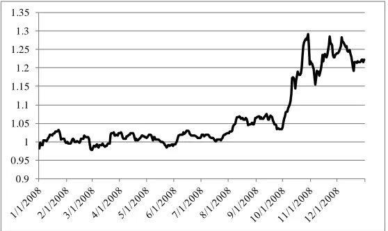
The unprecedented events in the latter part of 2008 also had significant effects on
exchange rates, as demand for U.S. dollars soared. For example, from September 15
through the end of 2008, the U.S. dollar rose over 15% relative to the Canadian dollar,
32% relative to the Brazilian real, and 30% relative to the Mexican peso. Figure 1.1
illustrates the spike in exchange rate volatility after mid-September 2008 at the time of
the Lehman Brothers announcement.
To better understand the burden of different stocks and markets to respond to
exchange rates, I conduct all my tests on individual stocks separately for all trading days
from January 1, 2008 through September 14, 2008 (“low exchange rate volatility”
period), and for all trading days from September 15, 2008 through December 31, 2008
(“high exchange rate volatility” period). The latter period tests offer a unique
13
particular note is the simulation of Grammig et al. (2008) showing that price discovery
inferences are dramatically affected by volatile exchange rates. The study of the latter
part of 2008 offers an important empirical test of the simulation conclusions.
1.4.B. Market Characteristics
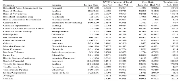
Tables 1.1 – 1.3 present market characteristics for each of the sampled stocks in Canada,
Brazil, and Mexico, respectively. The tables report the company name, industry
affiliation, NYSE listing date, NYSE volume as a percentage of total volume trading on
the two exchanges, relative cost ratio, and USD total assets. NYSE % Volume of Total
equals the U.S. dollar value of trading volume on the NYSE divided by the combined
U.S. dollar value of trading volume on the NYSE and the home exchange. A percentage
above 50% indicates that greater volume traded on the NYSE relative to the home
exchange. Cost Ratio is calculated as follows: for each exchange, for each minute, I
calculate the percent bid-ask spread equal to the ask price minus the bid price, divided by
the midpoint of the two prices. The Cost Ratio equals the percent bid-ask spread for the
home exchange divided by the percent bid-ask spread for the NYSE exchange. A Cost
Ratio above one indicates spreads are relatively larger on the home exchange versus the
NYSE. Sample-wide averages and medians are presented at the bottom of each table.
Results for the Canadian sample indicate that, on average, trading volume was
higher on the TSE (NYSE % Volume of Total was less than 50% for most of the stocks),
and bid-ask spreads were smaller (Cost Ratio was less than 1 for most of the stocks).
These findings indicate that the TSE maintained a cost and trading volume advantage
14
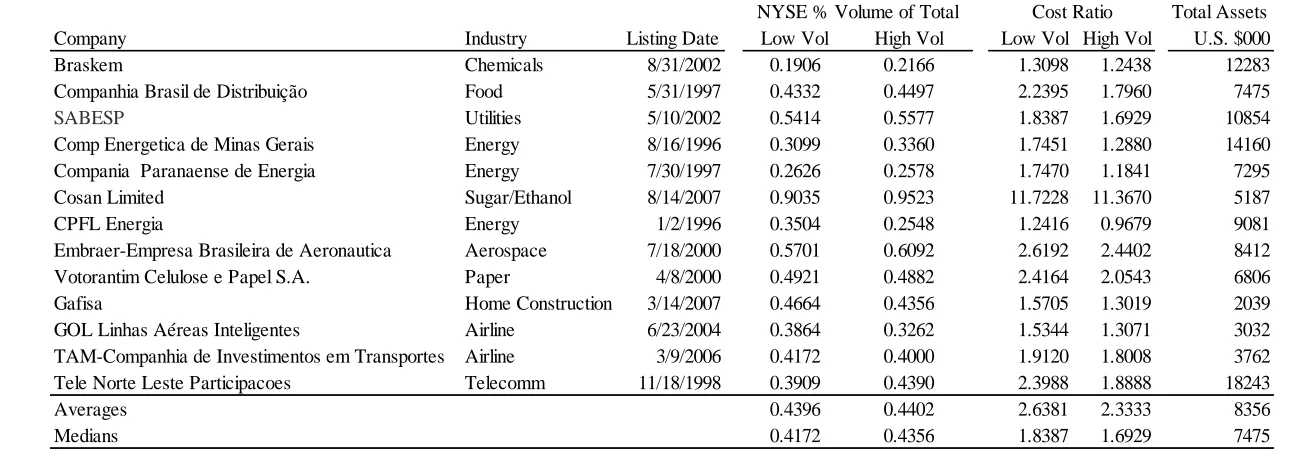
For the Brazilian sample (Table 1.2), trading volume and percent bid-ask spreads
were lower on the NYSE for most stocks. Cosan Limited stands out as an outlier, in
which most of the trading occurred on the NYSE. Therefore, the abnormal cost ratio for
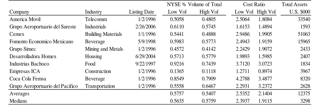
Cosan Limited is not meaningful. For the Mexican sample (Table 1.3), trading volume is
higher, and the percent bid-ask spreads are lower on the NYSE for most stocks.
In summary, the three markets exhibit wide differences in characteristics. For
Canadian cross-listings, the TSE dominates the NYSE on both trading volume and cost.
For Brazilian ADRs, trading volume favors the BOVESPA, but cost favors the NYSE.
And, for Mexican ADRs, both trading volume and cost favor the NYSE. The lack of
dominance of the home market for Mexico and Brazil adds to the robustness of our tests,
and offers a major contrast with existing studies of cross-listing price discovery (Ding et
al. (1999), Solnik (1996), Lieberman et al. (1999), Bacidore and Sofianos (2002), Wang
(2002), and Eun and Sabherwal (2003a, 2003b), and Harris et al. (2007)). Not
surprisingly, cross-listing studies of dominant home markets find that home markets also
dominate the price discovery process. However, the robustness of price discovery tests is
weakened when restricted to dominant home markets.
1.4.C. Cointegration Tests
Before estimating the vector error correction model, I determine the number of lags in the
model using the Schwarz Bayesian Information Criterion (Schwarz (1978)). Then, I use
Johansen’s (1988) method to test for cointegration, and confirm that there is only one
cointegrating vector. 7 The results of the Johansen’s (1988) rank test method support the hypothesis of one cointegrating vector among the three price series (prices at home,
7 Critical values (for models where the cointegrating vector is (n1) and
15
prices on the NYSE, and the exchange rate). The cointegrating vectors are estimated
using Johansen’s (1995) maximum likelihood method and are reported in Tables 1.4 to
1.6. The results offer strong support for the theoretical values discussed in section II.C.
The median cointegrating vectors, rounded to two decimal places, are (1.00,-1.00,-1.00)
over both periods for all countries. This finding indicates that prices converge after
adjusting for exchange rates. The prices do not deviate without bound, and subsequently
tend to correct toward each other.
1.4.D. Impulse Response Functions
The vector moving average ψ matrices form the basis of analysis to show the time
evolution of the effect on stock prices of a one-time shock to exchange rates. One might
suspect that because the NYSE is a derivative or satellite market relative to the home
market, that the NYSE will bear most of the adjustment to exchange rate changes.
However, the NYSE is the most liquid, transparent, and recognized exchange in the
world and the U.S. is a leading financial center and importer of foreign goods. In this
case, NYSE prices might offer information to which the home market responds.
Therefore, it is unclear the extent to which the NYSE will bear the burden to adjust to
exchange rate shocks. Only the empirical analysis can reveal the true relations.
I simulate the vector error correction models to derive impulse response functions
(IRF) for each stock. The IRFs illustrate the impact on stock prices of a 1-time, 1-unit
increase to EH US/ ; i.e., a depreciation in the home currency relative to the U.S. dollar, or,
alternatively, an appreciation of the U.S. dollar relative to the home currency. The Ψ(1)
matrix consists of the permanent effects (i.e., the values to which the impulse response
16
IRFs for each of the sampled stocks, I plot the IRF for three stocks for each market: the
stocks with the smallest, median, and largest translation risk percentage (TRP).
Figure 1.2 illustrates the IRFs. Each IRF extends 500 steps ahead. Each step
represents 1 minute in time. A positive shock to EH US/ is expected to cause stock prices to
rise in the home exchange and/or to fall on the NYSE. The left side panel presents IRFs
for stocks with the smallest TRP within Brazil, Mexico, and Canada, respectively. The
middle panel presents IRFs for stocks with the median TRP within each market. The
right side panel presents IRFs for stocks with the largest TRP within each market. TRP
equals the burden of the NYSE price to adjust to changes in exchange rates, relative to
the combined adjustment of the NYSE and home exchanges. The exact response for each
stock is determined by the TRP for the stock. A high TRP indicates that the NYSE prices
bear most of the burden to adjust to the exchange rate shock (the right side IRFs for each
market in Figure 1.2). A low TRP indicates that the NYSE prices bear little of the burden
to adjust to the exchange rate shock (the left side IRFs for each market in Figure 1.2).
Very interesting patterns emerge in the IRFs. In contrast to claims made on
limited samples by Grammig et al. (2005) and Frijns et al. (2010), my findings show that
stocks do not respond similarly to exchange rate shocks. In particular, the left and right
side panels reveal stark contrasts, illustrating dramatic differences in responses of prices
to the exchange rate shock. The middle panel offers the median tendency for each
country, and illustrate how New York prices tend to respond more than home prices to
the exchange rate shocks for Canadian and Mexican securities, and how home prices are
17
rate shock are persistent – the impacts level off after about 20 to 50 minutes (which is
similar to the findings of Eun and Sabherwal (2003) and Grammig et al. (2005)).8
1.4.E. Permanent Impulse Response Coefficients
The elements of the Ψ(1) matrix consist of the permanent impulse response coefficients
or price impact coefficients. HOME E, is the home price impact associated with exchange
rate changes, and NYSE E, is the NYSE price impact associated with exchange rate
changes. If I find that ˆNYSE E, ˆHOME E, (e.g., TRP > 50%), then I can conclude that the NYSE bears over half of the exchange rate burden. In their study of three blue chip
German stocks, Grammig et al. (2005) find that “New York prices bear almost all of the
adjustment to exchange rate changes” (p 162). But, little is known about pricing
dynamics for cross-listings domiciled in less dominant home stock markets such as
Mexico and Brazil. There is little reason to believe that the brief overlapping trading
results for three blue chip German stocks can be generalized for all stocks for all markets.
Paired coordinates for HOME E, and NYSE E, are graphed in Figure 1.3. For each
firm, HOME E, is graphed on the Y-axis and NYSE E, is graphed on the X-axis. Points that fall near the 45 degree line indicate a more symmetric response to exchange rate shocks
(i.e., equal burden for the NYSE versus home prices to adjust to exchange rate shocks).
8 Eun and Sabherwal (2003) examine an equally-weighted portfolio of Canadian cross-listings, and find
18
Points that fall below the 45 degree line correspond to firms in which NYSE prices bore
the larger burden to adjust to exchange rates.
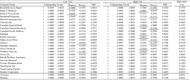
Five findings emerge from the psi estimates in Tables 1.4 – 1.6 and Figure 1.3.
For the time being I focus on the sample-wide results. Discussion of country-specific
findings will be offered when I discuss the results reframed as TRPs. First, Tables 1.4 –
1.6 show that all estimates have the expected signs: ˆHOME E, values are positive and
, ˆNYSE E
are negative for every stock.9 Second, Figure 1.3 shows that the ψ estimates are
widely dispersed across stocks within the same market, implying that the burden to adjust
to exchange rates is a stock specific effect, and not a market-wide effect. Third, the ψ
estimates in Figure 1.3 rarely lie close to the 45 degree line, implying that the NYSE and
home burden to adjust to exchange rates is similar only in rare cases. Fourth, the
dispersion of the ψ estimates in Figure 1.3 widens during the high exchange rate volatility
period within each market. The increased dispersion may be attributable to increased
dispersion in stock specific characteristics such as bid-ask spreads and trading volume,
but also may be attributable to the dramatic rise in exchange rate volatility.10 And, fifth, the NYSE bears less of the exchange rate burden for a substantial number of firms.
Specifically, 21 of the 46 points (46%) lie above the 45 degree line in the low exchange
rate volatility period, and 19 of the 46 points (41%) lie above the 45 degree line in the
9
,
HOME E
is the response of the home stock price to a 1-unit shock in the home price of one U.S. dollar (
/
H US
E ), and NYSE E, is the response of the New York price to a 1-unit shock in EH US/ . A 1-unit shock in
/
H US
E implies a depreciation (appreciation) of the home (U.S. dollar) currency versus the U.S. dollar (home currency). Therefore, in response to the EH US/ shock, we should expect the home exchange price to rise,
, ˆHOME E 0,
and/or the New York price to fall ˆNYSE E, 0 to meet the new equilibrium price.
10 Sample-wide medians presented in Tables 1.1 – 1.3 indicate trading volume and cost variables are fairly
19
high exchange rate volatility period. This finding contrasts others that claim that the
NYSE should bear all of the exchange rate burden.
The results show that both price series respond to exchange rate shocks. In order
to compare the magnitudes of the HOME E, and NYSE E, estimates, I perform likelihood
ratio tests to test the null hypothesis that HOME E, = NYSE E, . The null hypothesis of
equality of the two psi estimates is rejected at the 5 percent level of significance for 34
(36) of the 46 firms during the period of low (high) exchange rate volatility. Of the 34
significant differences during the period of low exchange rate volatility, 14 are positive
and 20 are negative. Of the 36 significant differences during the period of high exchange
rate volatility, 13 are positive and 23 are negative. Also, when averaging over the total
sample of 46 cross-listings, I conducted a paired t-test that controls for cross-correlation
in the psi estimates. The t-statistic for equality of sample-wide averages,
, , 0
HOME E NYSE E
, equals -1.84 (p-value = 0.072) for the period of high exchange
rate volatility, equals -1.72 (p-value = 0.092) for the period of low exchange rate
volatility, and equals -2.49 (p-value = 0.014) when combining both periods. A negative
difference indicates that the NYSE burden (NYSE E, ) to adjust to exchange rates is larger
in magnitude than the home exchange burden (HOME E, ).
In Figure 1.4, I compare the combined markets’ burden to adjust to exchange rate
shocks during the low versus the high exchange rate volatility periods. The sum of
,
HOME E
and NYSE E, measures the combined burden of the home market and the NYSE
20
calculated for the high exchange rate volatility period is graphed on the X-axis. Points
that lie below the 45 degree line signify firms that experienced an increase in the
combined markets’ burden to adjust to exchange rates during the period of high exchange
rate volatility.
As illustrated in Figure 1.4, the overall burden of adjusting to exchange rate
shocks (the sum of ˆHOME E, and the absolute value of ˆNYSE E, ) increased during the period
of high exchange rate volatility for the majority of firms. Specifically, the overall burden
rose for 31 of the 46 firms, (t-statistic for difference of percentage from 50% equals
2.52). Therefore, the dramatic rise in exchange rate volatility had a likewise dramatic
effect on the combined burdens of stock prices in the two markets to adjust to exchange
rate shocks.
Results of the TRP tests are reported in Tables 1.4 – 1.6, for Canada, Brazil, and
Mexico, respectively. For the Canadian results in Table 1.4, the mean (median) TRP
equals 59% (69%) versus 62% (71%) for the period of low versus high exchange rate
volatility. The coefficients exhibit wide cross-sectional variation, with a standard
deviation of 0.27 for the period of low exchange rate volatility, and 0.32 for the period of
high exchange rate volatility. The NYSE burden exceeds the home burden for 65% (61%)
of the sample during the period of low (high) exchange rate volatility. Both percentages
significantly exceed 50% (t-statistics for difference from 50% equal 3.42 and 2.33,
respectively). And, the psi estimates are statistically significant at the 5% level in nearly
every case. These results confirm that, while the NYSE bore more of the burden, both
markets bore significant burdens to adjust to exchange rate shocks. In contrast, Grammig
21
burden of adjustment to exchange rate changes. My tests show that these earlier claims
are sample specific, and, therefore, the generalizations are misleading. When examining a
more robust set of firms, I find that the burden of prices to adjust to exchange rates is not
borne primarily by the foreign market.
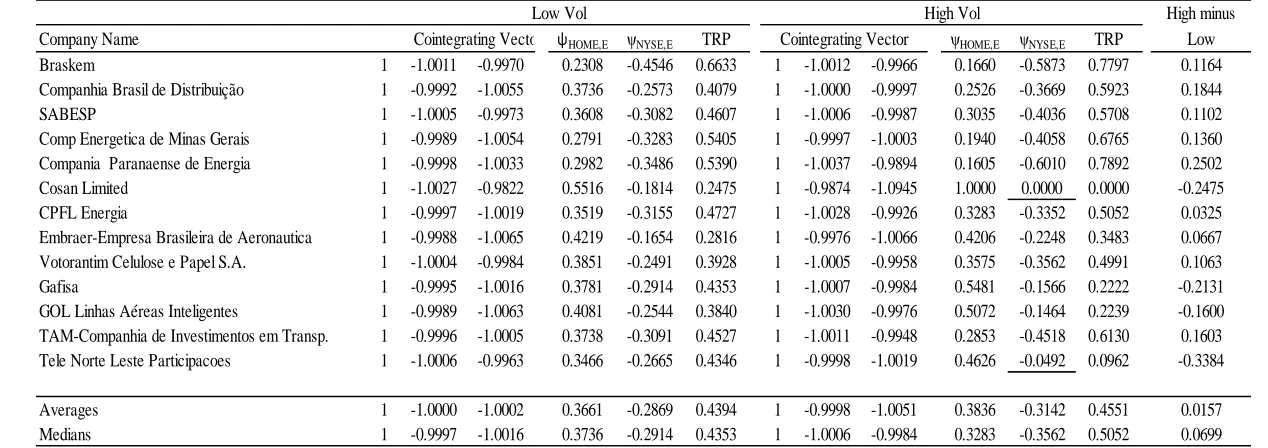
Results for the Brazilian sample differ markedly from the Canadian results. For
the Brazilian results in Table 1.5, the mean (median) TRP equals 44% (44%) versus 47%
(50%) when comparing the periods of low versus high exchange rate volatility.11 Relative to the Canadian results, the TRPs are more closely clustered (standard deviations of 0.11
and 0.24 for the periods of low and high exchange rate volatility, respectively). Thus,
there is considerably more homogeneity among the TRPs for the Brazilian sample versus
the Canadian sample. The NYSE burden exceeds the home burden only 23% of the time
during the period of low exchange rate volatility (significantly less than 50%; t-statistic
for difference from 50% equals -5.47). This percentage rises to 51% during the period of
high exchange rate volatility. The Brazilian results indicate that, relative to BOVESPA
prices, NYSE prices bear far less of the burden to adjust to exchange rate shocks during
the low exchange rate volatility period, but that the burden was fairly evenly shared
during the high exchange rate volatility period. It should be noted that most of the psi
estimates are significant at the 5% level in each period, once again implying that both
markets bore at least part of the exchange rate burden.
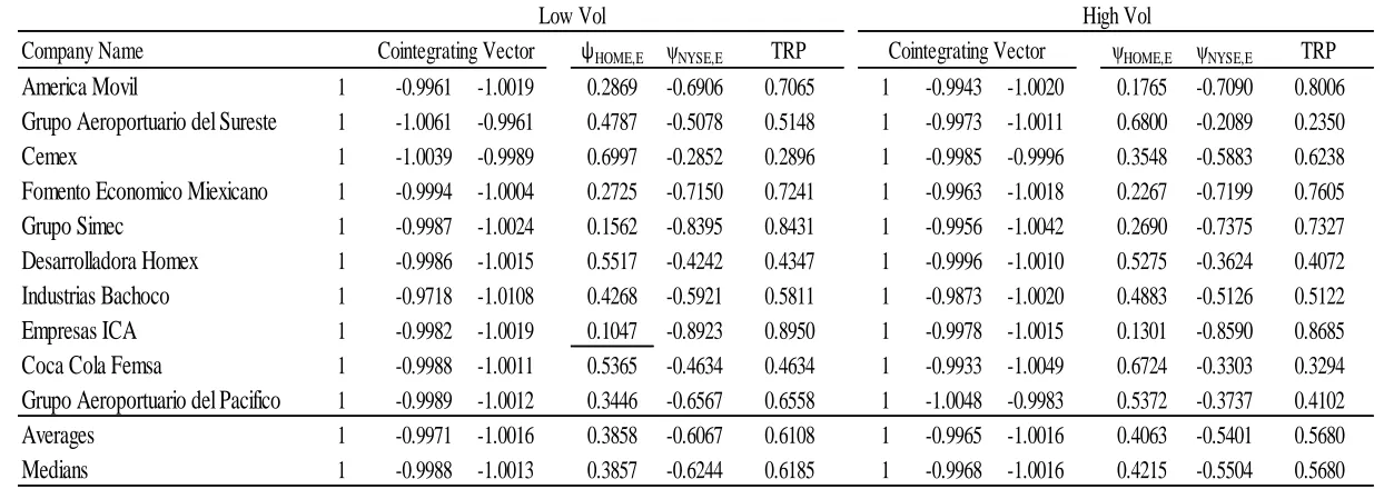
The Mexican sample results are reported in Table 1.6. The mean (median) TRP
equals 61% (62%) versus 57% (57%) for the periods of low versus high exchange rate
11 Cosan Limited offers an interesting case study. From Table 1.5, it is clear that most trading in Cosan
22
volatility. The Mexican results exhibit more homogeneity than the Canadian results
(standard deviation approximately 0.20 in each period). The NYSE burden exceeds the
home burden 70% of the time during the low exchange rate volatility period
(significantly greater than 50%; t-statistic for difference from 50% equals 3.01), and 60%
of the time during the high exchange rate volatility period (t-statistic for difference from
50% equals 1.32). In general, tests on Mexican cross-listings show that the NYSE
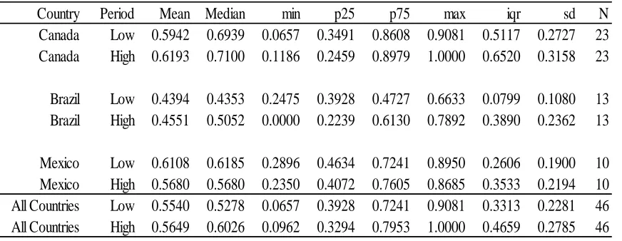
investor bears more of the exchange rate burden than the home investor. Summary
statistics for the TRP estimates for the three markets are provided in Table 1.7.
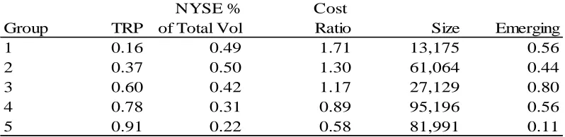
1.4.F. Cross-Sectional TRP Tests
Table 1.8 reports averages for quintile portfolios formed based on TRP (the translation
risk percentage defined in Equation (1.12), which measures the relative burden of the
NYSE price to adjust to exchange rate shocks. Quintile 1 consists of the lowest TRP
quintile, and quintile 5 consists of the largest TRP quintile. NYSE % Volume of Total
equals the trading volume in USD divided by the sum of the USD denominated trading
volume on both the NYSE and home exchange. The Cost Ratio equals the percentage
bid-ask quote spread on the home exchange divided by the percentage bid-ask quote
spread on the NYSE. Size equals total assets in thousands USD. Emerging equals the
percentage of the group consisting of emerging market stocks. While small sample
caveats are in order, it is important to note that my sample size is among the largest of
any high frequency price discovery study.
The quintile results reveal interesting monotonic patterns. The NYSE’s relative
share of total trading volume generally falls from TRP quintile 1 through TRP quintile 5.
23
Although not as clear, size is larger for the higher TRP quintiles than for the lower TPR
quintiles. If size is a proxy for familiarity, then our results suggest that the NYSE share of
the exchange rate burden is higher for the more familiar firms. The final column shows
that TRP quintile 5 consists mainly of Canadian stocks (the emerging market composition
in quintile 5 is well below 50%). In summary, the results show that the NYSE share of
the exchange rate burden tends to be higher for larger firms, and for those with lower
trading volumes on the NYSE relative to the home market, and lower costs on the home
exchange relative to the NYSE.
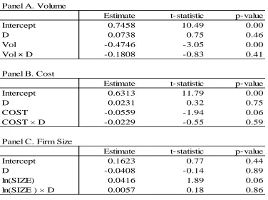
I also run cross-sectional regressions of TRP against NYSE % of Total Volume,
Cost Ratio, and the natural logarithm of total assets. The regressions are run individually
to avoid multicollinearity problems that exist especially between COST and VOL. The
regressions pool the data across both time periods, and include an interaction dummy
variable to measure changes in slopes between the low and high exchange rate volatility
periods.
Results are consistent with the quintile results. The VOL slope coefficient is
significant at the 0.05 level, and COST and SIZE slope coefficients are significant at the
0.10 level. The signs of the slopes are consistent with the quintile results; namely that
TRP is negatively related to both VOL and COST, and is positively related to SIZE.
Slope coefficients intensify during the period of high exchange rate volatility (i.e., the
signs on the interaction terms are identical to the variable’s coefficients), however, the
interaction term coefficients are not statistically significant.
1.5. Conclusions
In this study, I examined the informational role of exchange rates in the price formation
24
price impacts of exchange rate shocks. Using a sample of 46 cross-listings on the NYSE
from Canada, Brazil, and Mexico during 2008, I found that New York prices bore
roughly 60% of the adjustment to exchange rates for Canadian and Mexican securities,
and roughly 45% for Brazilian securities. These findings showed that price adjustments
from exchange rate shocks transpired on both the home exchange and the NYSE.
Therefore, it is not the case that foreign prices (e.g., NYSE prices) bear nearly all the
burden to adjust to exchange rates, as suggested in existing studies that examine less
diverse sets of stocks and markets.
Findings varied considerably across firms, indicating that the effects of exchange
rate shocks are not market-based, but more likely are firm-specific. For the majority of
firms, the combined markets’ burdens to adjust to exchange rate shocks rose during the
period of high exchange rate volatility. This finding suggests that traditional price
discovery measures such as Hasbrouck’s (1995) information shares become increasingly
affected by exchange rate effects versus firm-specific fundamental news effects during
periods of increasing exchange rate volatility.
Cross-sectional tests revealed that the NYSE burden to adjust to exchange rate
changes is highest for big firms, and for those with relatively low NYSE trading volume,
or with high NYSE trading costs. The findings indicate that the burden to adjust to
exchange rates is likely to shift more to emerging market exchanges as the migration of
trading volume to the NYSE increases. The results also have important implications for
international price discovery tests, especially for those that fail to model an independent
25
Table 1.1
Canadian Sample Summary
This table lists the Canadian companies by name, industry, NYSE listing date, relative trading volume, cost, and size. The low exchange rate volatility period (Low Vol) spans all trading days in January 1, 2008 – September 14, 2008. The high exchange rate volatility period (High Vol) spans all trading days in September 15, 2008 – December 31, 2008. September 15, 2008 is the date of the Lehman Brother. bankruptcy declaration and the start of market turmoil and volatility.
Total As s ets
Company Indus try Lis ting Date Low Vol High Vol Low Vol High Vol U.S. $000
Brookfield As s et Management Inc Financial 7/10/1998 0.3360 0.3804 1.1040 0.8152 57430
Bank of Montreal Banking 10/5/2005 0.0805 0.0715 0.6086 0.4478 366538
Bank of Nova Scotia Banking 1/2/1996 0.0737 0.0507 0.5815 0.4143 449944
Brookfield Properties Corp Real Es tate 1/2/1996 0.6240 0.6728 1.4088 1.0432 20391 Biovail Corporation International Pharmaceuticals 6/2/1999 0.3625 0.3074 1.1755 1.1456 1732 Celes tica Inc. Electronics Manufacturing 5/10/2000 0.3844 0.2965 1.1867 1.1974 4457
Canadian Imperial Bank Banking 7/1/1998 0.0764 0.0814 0.5530 0.4541 330593
Canadian Natural Res ources Limited Oil and Gas 1/2/1996 0.2657 0.2185 0.8285 0.5369 37576 Canadian Pacific Railway Trans portation 2/1/2003 0.2604 0.3284 0.7976 0.7224 13292
Enbridge Inc. Oil and Gas 1/2/1996 0.1578 0.1738 0.7178 0.5462 20215
Fairfax Financial Ins urance 6/6/1997 0.3616 0.2812 0.8904 0.5605 27565
Gildan ActiveWear Apparel 10/30/2001 0.3290 0.3586 1.0177 0.9185 8670
Gains co Ins urance 7/23/1996 0.4181 0.3560 1.0523 0.8650 1053
Manulife Financial Financial Services 6/10/1998 0.1777 0.1313 0.9005 0.5501 350553
Nova Chemicals Chemicals 7/31/1996 0.4185 0.3724 1.0238 0.8567 4914
Northern Telecom Switching equipment 3/9/1996 0.4589 0.3033 1.1744 0.7102 16315
Nexen Inc Oil and Gas 7/11/1998 0.2071 0.2030 0.8866 0.6019 19731
Ritchie Brothers Auctioners Indus trial Equipment 1/1/1996 0.6341 0.5499 1.6196 1.5255 841
Sun Life Financial Ins urance 11/14/2000 0.1518 0.1028 0.7054 0.5585 184485
Toronto Dominion Bank Banking 11/14/2002 0.1641 0.1084 0.8538 0.5283 497902
Tim Hortons Inc Res taurant 1/2/1996 0.3509 0.3437 1.2430 0.9756 1737
Trans Canada Pipeline Oil and Gas 8/30/1996 0.0846 0.1093 0.6679 0.5258 31022
Domtar Corporation Paper Products 3/22/2006 0.7798 0.8917 1.8711 2.0779 7631
Averages 0.3112 0.2910 0.9943 0.8077 106721
Medians 0.3290 0.2965 0.9005 0.7102 20215
26
Table 1.2
Brazilian Sample Summary
This table lists the Brazilian companies by name, industry, and NYSE listing date and relative trading volume, cost, and price characteristics. NYSE % Volume of Total is trading volume expressed in USD on the NYSE divided by the USD denominated trading volume on both the NYSE and the BOVESPA. The percentage bid-ask quote equals the ask price minus the bid price, divided by the midpoint of the two prices. The percentage bid-ask quote is calculated for every 1-minute interval, for each stock. For each minute, the Cost Ratio equals the percentage quote spread on the home exchange divided by the percentage quote spread on the NYSE. To calculate the exchange rate adjusted home stock price quote, for each minute, the midpoint of the 1-minute exchange rate bid and ask price quotes is multiplied times the midpoint of the home stock bid and ask price.
Total Assets Company Industry Listing Date Low Vol High Vol Low Vol High Vol U.S. $000 Braskem Chemicals 8/31/2002 0.1906 0.2166 1.3098 1.2438 12283 Companhia Brasil de Distribuição Food 5/31/1997 0.4332 0.4497 2.2395 1.7960 7475
SABESP Utilities 5/10/2002 0.5414 0.5577 1.8387 1.6929 10854
Comp Energetica de Minas Gerais Energy 8/16/1996 0.3099 0.3360 1.7451 1.2880 14160 Compania Paranaense de Energia Energy 7/30/1997 0.2626 0.2578 1.7470 1.1841 7295 Cosan Limited Sugar/Ethanol 8/14/2007 0.9035 0.9523 11.7228 11.3670 5187 CPFL Energia Energy 1/2/1996 0.3504 0.2548 1.2416 0.9679 9081 Embraer-Empresa Brasileira de Aeronautica Aerospace 7/18/2000 0.5701 0.6092 2.6192 2.4402 8412 Votorantim Celulose e Papel S.A. Paper 4/8/2000 0.4921 0.4882 2.4164 2.0543 6806 Gafisa Home Construction 3/14/2007 0.4664 0.4356 1.5705 1.3019 2039 GOL Linhas Aéreas Inteligentes Airline 6/23/2004 0.3864 0.3262 1.5344 1.3071 3032 TAM-Companhia de Investimentos em Transportes Airline 3/9/2006 0.4172 0.4000 1.9120 1.8008 3762 Tele Norte Leste Participacoes Telecomm 11/18/1998 0.3909 0.4390 2.3988 1.8888 18243
Averages 0.4396 0.4402 2.6381 2.3333 8356
Medians 0.4172 0.4356 1.8387 1.6929 7475
27
Table 1.3
Mexican Sample Summary
This table lists the Mexican companies by name, industry, and NYSE listing date and relative trading volume, cost, and price characteristics. NYSE % Volume of Total is trading volume expressed in USD on the NYSE divided by the USD denominated trading volume on both the NYSE and the BOLSA. The percentage bid-ask quote equals the ask price minus the bid price, divided by the midpoint of the two prices. The percentage bid-ask quote is calculated for every 1-minute interval, for each stock. For each minute, the Cost Ratio equals the percentage quote spread on the home exchange divided by the percentage quote spread on the NYSE. To calculate the exchange rate adjusted home stock price quote, for each minute, the midpoint of the 1-minute exchange rate bid and ask price quotes is multiplied times the midpoint of the home stock bid and ask price.
Total Assets Company Industry Listing Date Low Vol High Vol Low Vol High Vol U.S. $000 America Movil Telecomm 1/2/1996 0.5058 0.4805 2.5064 1.8084 33540 Grupo Aeroportuario del Sureste Industrials 2/26/2006 0.6110 0.5745 1.6153 1.4894 1593 Cemex Building Materials 1/1/1996 0.5441 0.4888 2.9486 1.9905 51063 Fomento Economico Mexicano Beverage 5/9/1998 0.5983 0.5773 2.4943 1.9159 15965 Grupo Simec Mining and Metals 1/2/1996 0.4572 0.4142 2.2429 1.9072 2433 Desarrolladora Homex Housing 6/29/2004 0.5713 0.5779 1.9893 1.5985 2407 Industrias Bachoco Food 9/22/1997 0.9216 0.7439 3.7120 3.0723 1834 Empresas ICA Construction 1/2/1996 0.1365 0.1118 1.2711 0.8974 3967 Coca Cola Femsa Beverage 1/2/1996 0.8549 0.7909 4.2788 3.4877 8320 Grupo Aeroportuario del Pacifico Transportation 1/2/1996 0.5558 0.6467 2.2931 3.2372 2628
Averages 0.5757 0.5407 2.5352 2.1404 12375
Medians 0.5635 0.5759 2.3937 1.9115 3298
28
Table 1.4
Exchange Rate Effects for the Canadian Sample
This table reports cointegrating vector coefficients and permanent foreign exchange impulse response coefficients for the Canadian stock sample. The ψHOME,E (ψNYSE,E) columns present impulse response coefficients measuring the effect that U.S. dollar to Canadian dollar exchange rate changes have on the TSE (NYSE) price of each stock. The TRP column presents the translation risk percent equal to the absolute value of the ψNYSE,E estimate divided by the sum of the estimates of ψHOME,E and absolute value ψNYSE,E. The final column presents differences in TRPs for the periods of high versus low exchange rate volatility.
All underlined coefficients are insignificant at the 5% level. All non-underlined coefficients are significant at the 5% level.
High minus
Company Name ψHOME,E ψNYSE,E TRP ψHOME,E ψNYSE,E TRP Low
Brookfield Asset Mgmt 1 -0.9995 -1.0025 0.1068 -0.7933 0.8814 1 -1.0000 -1.0005 0.7081 -0.1002 0.1240 -0.7574 Bank of Montreal 1 -1.0000 -0.9998 0.1244 -0.7214 0.8529 1 -0.9998 -1.0045 0.0867 -0.8924 0.9114 0.0585 Bank of Nova Scotia 1 -1.0000 -1.0007 0.0674 -0.6660 0.9081 1 -0.9999 -1.0020 0.1571 -0.7857 0.8334 -0.0748 Brookfield Properties 1 -1.0000 -0.9994 0.5495 -0.2947 0.3491 1 -0.9998 -1.0019 0.7139 -0.1113 0.1349 -0.2142 Biovail Corporation Int'l 1 -1.0000 -0.9994 0.4757 -0.3525 0.4256 1 -1.0002 -1.0013 0.5312 -0.3712 0.4113 -0.0143 Celestica Inc. 1 -1.0001 -1.0008 0.6717 -0.2287 0.2540 1 -0.9998 -1.0015 0.3014 -0.7050 0.7005 0.4465 Canadian Imperial Bank 1 -1.0000 -1.0005 0.1946 -0.5038 0.7213 1 -0.9996 -1.0043 0.0000 -1.0000 1.0000 0.2787 Canadian Natural Resources 1 -1.0000 -0.9997 0.1751 -0.6906 0.7977 1 -1.0000 -1.0000 0.6640 -0.2146 0.2443 -0.5535 Canadian Pacific Railway 1 -1.0000 -1.0004 0.4497 -0.2714 0.3763 1 -1.0000 -0.9988 0.4485 -0.4386 0.4944 0.1181 Enbridge 1 -1.0000 -0.9997 0.1933 -0.4593 0.7039 1 -1.0002 -0.9990 0.0853 -0.7347 0.8959 0.1921 Fairfax Financial 1 -1.0000 -0.9920 0.3865 -0.5468 0.5859 1 -0.9994 -1.0094 0.0672 -0.9502 0.9340 0.3481 Gildan ActiveWear 1 -1.0000 -1.0001 0.1263 -0.7810 0.8608 1 -1.0002 -0.9959 0.8476 -0.1141 0.1186 -0.7421 Gainsco 1 -1.0000 -1.0028 0.7518 -0.0529 0.0657 1 -0.9997 -0.9925 0.7941 -0.1256 0.1366 0.0708 Manulife Financial 1 -1.0000 -1.0012 0.4988 -0.1595 0.2423 1 -0.9998 -1.0051 0.2555 -0.6254 0.7100 0.4676 Nova Chemicals 1 -1.0000 -0.9979 0.3715 -0.4628 0.5547 1 -1.0001 -0.9959 0.1016 -0.8933 0.8979 0.3432 Northern Telecom 1 -1.0000 -0.9975 0.7571 -0.1284 0.1450 1 -1.0053 -0.9291 0.0358 -0.9125 0.9622 0.8172 Nexen Inc 1 -1.0000 -1.0020 0.0920 -0.8156 0.8986 1 -1.0000 -1.0033 0.0879 -0.8687 0.9081 0.0095 Ritchie Brothers Auctioners 1 -1.0000 -0.9982 0.1217 -0.8028 0.8683 1 -0.9999 -1.0017 0.2015 -0.7829 0.7953 -0.0730 Sun Life Financial 1 -1.0000 -1.0005 0.1809 -0.6515 0.7827 1 -1.0000 -0.9989 0.3173 -0.6776 0.6811 -0.1016 Toronto Dominion Bank 1 -1.0000 -0.9997 0.2365 -0.5363 0.6939 1 -0.9999 -1.0031 0.4287 -0.3619 0.4577 -0.2362 Tim Hortons Inc 1 -1.0000 -0.9987 0.4018 -0.4292 0.5165 1 -0.9999 -1.0006 0.1416 -0.8104 0.8513 0.3348 TransCanada Pipeline 1 -1.0000 -1.0000 0.0911 -0.6828 0.8823 1 -1.0001 -1.0017 0.1989 -0.7724 0.7952 -0.0871 Domtar Corporation 1 -1.0000 -1.0009 0.6204 -0.2641 0.2986 1 -1.0003 -0.9952 0.7485 -0.2441 0.2459 -0.0527 Averages 1 -1.0000 -0.9998 0.3324 -0.4911 0.5942 1 -1.0002 -0.9977 0.3444 -0.5866 0.6193 0.0251 Medians 1 -1.0000 -1.0000 0.2365 -0.5038 0.6939 1 -1.0000 -1.0013 0.2555 -0.7050 0.7100 0.0161
Cointegrating Vector Cointegrating Vector
29
Table 1.5
Exchange Rate Effects for the Brazilian Sample
This table reports cointegrating vector coefficients and permanent foreign exchange impulse response coefficients for the Brazilian stock sample. The ψHOME,E (ψNYSE,E) columns present impulse response coefficients measuring the effect that U.S. dollar to Brazilian real exchange rate changes have on the BOVESPA (NYSE) price of each stock. The TRP column presents the translation risk percent equal to the absolute value of the ψNYSE,E estimate divided by the sum of the estimates of ψHOME,E and absolute value ψNYSE,E. TRP equals the adjustment borne by the NYSE relative to the total adjustment from both markets in response to changes in the U.S. dollar to Brazilian real exchange rate. The final column presents differences in TRPs for the periods of high versus low exchange rate volatility.
All underlined coefficients are insignificant at the 5% level. All non-underlined coefficients are significant at the 5% level.
High minus Company Name ψHOME,E ψNYSE,E TRP ψHOME,E ψNYSE,E TRP Low
Braskem 1 -1.0011 -0.9970 0.2308 -0.4546 0.6633 1 -1.0012 -0.9966 0.1660 -0.5873 0.7797 0.1164 Companhia Brasil de Distribuição 1 -0.9992 -1.0055 0.3736 -0.2573 0.4079 1 -1.0000 -0.9997 0.2526 -0.3669 0.5923 0.1844 SABESP 1 -1.0005 -0.9973 0.3608 -0.3082 0.4607 1 -1.0006 -0.9987 0.3035 -0.4036 0.5708 0.1102 Comp Energetica de Minas Gerais 1 -0.9989 -1.0054 0.2791 -0.3283 0.5405 1 -0.9997 -1.0003 0.1940 -0.4058 0.6765 0.1360 Compania Paranaense de Energia 1 -0.9998 -1.0033 0.2982 -0.3486 0.5390 1 -1.0037 -0.9894 0.1605 -0.6010 0.7892 0.2502 Cosan Limited 1 -1.0027 -0.9822 0.5516 -0.1814 0.2475 1 -0.9874 -1.0945 1.0000 0.0000 0.0000 -0.2475 CPFL Energia 1 -0.9997 -1.0019 0.3519 -0.3155 0.4727 1 -1.0028 -0.9926 0.3283 -0.3352 0.5052 0.0325 Embraer-Empresa Brasileira de Aeronautica 1 -0.9988 -1.0065 0.4219 -0.1654 0.2816 1 -0.9976 -1.0066 0.4206 -0.2248 0.3483 0.0667 Votorantim Celulose e Papel S.A. 1 -1.0004 -0.9984 0.3851 -0.2491 0.3928 1 -1.0005 -0.9958 0.3575 -0.3562 0.4991 0.1063 Gafisa 1 -0.9995 -1.0016 0.3781 -0.2914 0.4353 1 -1.0007 -0.9984 0.5481 -0.1566 0.2222 -0.2131 GOL Linhas Aéreas Inteligentes 1 -0.9989 -1.0063 0.4081 -0.2544 0.3840 1 -1.0030 -0.9976 0.5072 -0.1464 0.2239 -0.1600 TAM-Companhia de Investimentos em Transp. 1 -0.9996 -1.0005 0.3738 -0.3091 0.4527 1 -1.0011 -0.9948 0.2853 -0.4518 0.6130 0.1603 Tele Norte Leste Participacoes 1 -1.0006 -0.9963 0.3466 -0.2665 0.4346 1 -0.9998 -1.0019 0.4626 -0.0492 0.0962 -0.3384
Averages 1 -1.0000 -1.0002 0.3661 -0.2869 0.4394 1 -0.9998 -1.0051 0.3836 -0.3142 0.4551 0.0157 Medians 1 -0.9997 -1.0016 0.3736 -0.2914 0.4353 1 -1.0006 -0.9984 0.3283 -0.3562 0.5052 0.0699
Low Vol High Vol
30
Table 1.6
Exchange Rate Effects for the Mexican Sample
This table reports cointegrating vector coefficients and permanent foreign exchange impulse response coefficients for the Mexican stock sample. The ψHOME,E (ψNYSE,E) columns present impulse response coefficients measuring the effect that U.S. dollar to Mexican peso exchange rate changes have on the BOLSA (NYSE) price of each stock. The TRP column presents the translation risk percent equal to the absolute value of the ψNYSE,E estimate divided by the sum of the estimates of ψHOME,E and absolute value ψNYSE,E. TRP equals the adjustment borne by the NYSE relative to the total adjustment from both markets in response to changes in the U.S. dollar to Mexican peso exchange rate. The final column presents differences in TRPs for the periods of high versus low exchange rate volatility.
All underlined coefficients are insignificant at the 5% level. All non-underlined coefficients are significant at the 5% level.
Company Name ψHOME,E ψNYSE,E TRP ψHOME,E ψNYSE,E TRP America Movil 1 -0.9961 -1.0019 0.2869 -0.6906 0.7065 1 -0.9943 -1.0020 0.1765 -0.7090 0.8006 Grupo Aeroportuario del Sureste 1 -1.0061 -0.9961 0.4787 -0.5078 0.5148 1 -0.9973 -1.0011 0.6800 -0.2089 0.2350 Cemex 1 -1.0039 -0.9989 0.6997 -0.2852 0.2896 1 -0.9985 -0.9996 0.3548 -0.5883 0.6238 Fomento Economico Miexicano 1 -0.9994 -1.0004 0.2725 -0.7150 0.7241 1 -0.9963 -1.0018 0.2267 -0.7199 0.7605 Grupo Simec 1 -0.9987 -1.0024 0.1562 -0.8395 0.8431 1 -0.9956 -1.0042 0.2690 -0.7375 0.7327 Desarrolladora Homex 1 -0.9986 -1.0015 0.5517 -0.4242 0.4347 1 -0.9996 -1.0010 0.5275 -0.3624 0.4072 Industrias Bachoco 1 -0.9718 -1.0108 0.4268 -0.5921 0.5811 1 -0.9873 -1.0020 0.4883 -0.5126 0.5122 Empresas ICA 1 -0.9982 -1.0019 0.1047 -0.8923 0.8950 1 -0.9978 -1.0015 0.1301 -0.8590 0.8685 Coca Cola Femsa 1 -0.9988 -1.0011 0.5365 -0.4634 0.4634 1 -0.9933 -1.0049 0.6724 -0.3303 0.3294 Grupo Aeroportuario del Pacifico 1 -0.9989 -1.0012 0.3446 -0.6567 0.6558 1 -1.0048 -0.9983 0.5372 -0.3737 0.4102 Averages 1 -0.9971 -1.0016 0.3858 -0.6067 0.6108 1 -0.9965 -1.0016 0.4063 -0.5401 0.5680 Medians 1 -0.9988 -1.0013 0.3857 -0.6244 0.6185 1 -0.9968 -1.0016 0.4215 -0.5504 0.5680
Cointegrating Vector Cointegrating Vector
31
Table 1.7
Summary Statistics for the NYSE Translation Risk Percentage
This table reports means, standard deviations (sd), interquartile ranges (iqr), and quartile results for TRPs for the sample of cross-listings from Canada, Brazil, and Mexico. TRP equals the burden of New York prices to adjust to exchange rate shocks expressed as a percent of the total burden of the NYSE and home market burdens. Results are presented separately for the period of low exchange rate volatility (January 1, 2008 – September 14, 2008) and high exchange rate volatility (September 15, 2008 – December 31, 2008).
Country Period Mean Median min p25 p75 max iqr sd N
Canada Low 0.5942 0.6939 0.0657 0.3491 0.8608 0.9081 0.5117 0.2727 23 Canada High 0.6193 0.7100 0.1186 0.2459 0.8979 1.0000 0.6520 0.3158 23
Brazil Low 0.4394 0.4353 0.2475 0.3928 0.4727 0.6633 0.0799 0.1080 13 Brazil High 0.4551 0.5052 0.0000 0.2239 0.6130 0.7892 0.3890 0.2362 13