Evaluation of three Simple Imputation Methods for
Enhancing Preprocessing of Data with Missing Values
ABSTRACT
One of the important stages of data mining is preprocessing, where the data is prepared for different mining tasks. Often, the real-world data tends to be incomplete, noisy, and inconsistent. It is very common that the data are not obtainable for every observation of every variable. So the presence of missing variables is obvious in the data set. A most important task when preprocessing the data is, to fill in missing values, smooth out noise and correct inconsistencies.
This paper presents the missing value problem in data mining and evaluates some of the methods generally used for missing value imputation. In this work, three simple missing value imputation methods are implemented namely (1) Constant substitution, (2) Mean attribute value substitution and (3) Random attribute value substitution.
The performance of the three missing value imputation algorithms were measured with respect to different rate or different percentage of missing values in the data set by using some known clustering methods. To evaluate the performance, the standard WDBC data set has been used.
Keywords:
Datamining, Preprocessing, Imputation methods, Missing Data, Values1.
INTRODUCTION
Often, in the real world, entities may have two or more representations in databases. Now-a-days data is not a mere data. But it is applied to generate useful information. Knowledge discovery(KDD) plays an important role in data analysis. When Data Mining is applied on a data warehouse, low quality data source may lead to a false analysis report. So, it is essential to apply cleaning process like filling up of missing value, removal of duplicate datasets, etc on a database before using it for data mining
1.1 Survey on Missing Value Imputation
Methods
Missing values i mp u t a t i o n is an actual yet challenging issue confronted in machine learning and data mining [2]. Missing values m a y generate bias a n d affect the quality of the mining outcome [3, 4]. However, most ma c h i n e learning algorithms are not well adapted to some application domains due to the difficulty with missing values, such as Web application. Most of the existing algorithms are designed under the assumption that there are no missing values in datasets. But in practice a reliable method for dealing with those missing values is necessary.
Missing values may appear either in conditional attributes or in class attribute (target attribute). There are many approaches to deal with missing values described in [6], for instance: (a) Ignore objects containing missing values; (b) Fill the missing value manually; (c) Substitute the missing values by a global constant or the mean of the objects; (d) Get the
most probable value to fill in the missing values. The first approach usually lost too much useful information, whereas the second one is time- consuming and expensive, so it is infeasible in many applications. The third approach assumes that all missing values are with the same value, probably leading to considerable distortions in data distribution. However, Han et al. 2000, Zhang et al. 2005 in [2, 6] express “The method of imputation, however, is a popular strategy. In comparison to other methods, it uses as more information as possible from the observed data to predict missing values”.
Traditional missing value imputation techniques can be roughly classified into parametric imputation e.g., the linear regression and non -parametric imputation e.g., non-parametric kernel-based regression method [20, 21, 22], Nearest Neighbor method [4, 6](NN). The parametric regression imputation is superior if a dataset can be adequately modeled parametrically, or if users can correctly specify the parametric forms for the dataset.
Non-parametric imputation algorithm, which can provide superior fit by capturing structure in the dataset (note that a misspecified parametric model cannot), offers a nice alternative if users have no idea on the actual distribution of a dataset. For example, the NN method is regarded as one of non-parametric techniques used to compensate for missing values in sample surveys [7]. And it has been successfully used in, for instance, U.S. Census Bureau and Canadian Census Bureau. What's more, using a non-parametric algorithm is beneficial when the form of relationship between the conditional attributes and the target attribute is not known a-priori [8].
In recent years, many researchers focused on the topic of imputing missing values. Chen and Chen [9] presented an estimating null value method, where a fuzzy similarity matrix is used to represent fuzzy relations, and the method is used to deal with one missing value in an attribute. Chen and Huang [10] constructed a genetic algorithm to impute in relational database systems. The machine learning methods also include auto associative neural network, decision tree imputation, and so forth. All of these are pre-replacing methods. Embedded methods include case-wise deletion, lazy decision tree, dynamic path generation and some popular methods such as C4.5 and CART. But, these methods are not a completely satisfactory way to handle missing value problems. First, these methods only are designed to deal with the discrete values and the continuous ones are discretized before imputing the missing value, which may lose the true characteristic during the convertion process from the continuous value to discretized one. Secondly, these methods usually studied the problem of missing covariates (conditional attributes).
Besides these imputation methods that are considered in this paper, there are also other statistical methods exist. Statistics -based methods include linear regression, replacement under same standard deviation, and mean-mode method. But these methods are not completely satisfactory ways to handle missing value problems. Magnani[11] has
R.S. Somasundaram
Research Scholar
Research and Development Centre Bharathiar University
Coimbatore, India
R. Nedunchezhian
Vice-Principal
Kalaignar Karunanidhi Institute of Technology
reviewed the main missing data techniques (MDTs), and revealed that statistical methods have been mainly developed to manage survey data and proved to be very effective in many situations. However, the main problem of these techniques is the need of strong model assumptions. Other missing data imputation methods include a new family of reconstruction problems for multiple images from minimal data[12], a method for handling inapplicable and unknown missing data[13] , different substitution methods for replacement of missing data values [14], robust Bayesian estimator [15], and nonparametric kernel classification rules derived from incomplete (missing) data [16]. Same as the methods in machine learning, the statistical methods, which handle continuous missing values with missing in class label are very efficient, are not good at handling discrete value with missing in conditional attributes.
1.2 Missing data
Missing attribute values: one or more of the attribute values may be missing both for examples in the training set and for objects which are to be classified
Missing data might occur because the value is not relevant to a particular case, could not be recorded when the data was collected, or is ignored by users because of privacy concerns[1]. If attributes are missing in any training set, the system may either ignore this object totally, try to take it into account by, for instance, finding what is the missing attribute's most probable value, or use the value "missing", "unknown" or "NULL" as a separate value for the attribute.
The problem of missing values has been investigated since many times ago[1]. The simple solution is to discard the data instances with some missing values[24]. A more difficult solution is to try to determine these values [25]. Several techniques to handle missing values have been discussed in the literature [1][2]
The only really satisfactory solution to missing data is good design, but good analysis can help mitigate the problems [1].
Problems caused by missing data
1. Loss of precision due to less data
2. Computational difficulties due to holes in the dataset 3. Bias due to distortion of the data distribution Approaches for handling missing data
Thomas Lumley says, there are (at least) two ways to work with missing data[1]
1. By analogy with deliberately missing data in survey samples, model the probability of being missing and use probability weighting to estimate complete-data summaries
2. Model the distribution of the missing data and use explicit imputation or maximum likelihood which does implicit imputation.
1.3 Handle Missing Values
Choosing the right technique is a choice that depends on the problem domain, the data‟s domain and our goal for the data mining process.
The different approaches to handle missing values in database are:
1. Ignore the data row
This is usually done when the class label is missing (assuming our data mining goal is classification), or many attributes are missing from the row (not just one). However you‟ll obviously get poor performance if the percentage of such rows is high. For example, let‟s say that we have a database of students
“Medium” and “High”. Lets say our goal is do build a model predicting a student‟s success in college. Data rows which are missing the success column are not useful in predicting success so they could very well be ignored and removed before running the algorithm.
2. Use a global constant to fill in for missing values
Decide on a new global constant value, like "unknown", "N/A", “Hypen” or infinity that will be used to fill all the missing values.
This technique is used because sometimes it just doesn‟t make sense to try and predict the missing value.
For example, in student‟s enrollment database, assuming the state of residence attribute data is missing for some students. Filling it up with some state doesn‟t really make sense as opposed to using something like “N/A”.
3. Use attribute mean
Replace missing values of an attribute with the mean (or median if its discrete) value for that attribute in the database. For example, in a database of US family incomes, if the average income of a US family is X you can use that value to replace missing income values.
4. Use attribute mean for all samples belonging to the same class
Instead of using the mean (or median) of a certain attribute calculated by looking at all the rows in a database, It may be limited to the calculations to the relevant class to make the value more relevant to the row considered.
In a cars pricing database that among other things, classifies cars to "Luxury" and "Low budget" and missing values is dealt in the cost field. Replacing missing cost of a luxury car with the average cost of all luxury cars is probably more accurate than the value that is computed by the factor in the low budget cars.
5. Use a data mining algorithm to predict the most probable value
The value can be determined using regression, inference based tools using Bayesian formalism, decision trees, clustering algorithms (K-Mean\Median etc.).
For example, we could use a clustering algorithms to create clusters of rows which will then be used for calculating an attribute mean or median as specified in technique #3. Another example could be using a decision tree to try and predict the probable value in the missing attribute, according to other attributes in the data.
1.4 Evaluating the quality of the result
clusters with Rand Index Measure
Validating clustering algorithms and comparing performance of different algorithms are complex because it is difficult to find an objective measure of quality of clusters. In order to compare results against external criteria, a measure of agreement is needed. Since we assume that each record is assigned to only one class in the external criterion and to only one cluster, measures of agreement between two partitions can be used
The Rand index or Rand measure is a commonly used technique for measure of such similarity between two data clusters.
Given a set of n objects S = {O1, ..., On} and two data clusters of S which we want to compare: X = {x1, ..., xR} and Y = {y1, ..., yS} where the different partitions of X and Y are disjoint and their union is equal to S; we can compute the following values:
a is the number of elements in S that are in the same partition in X and in the same partition in Y,
c is the number of elements in S that are in the same partition in X and not in the same partition in Y,
d is the number of elements in S that are not in the same partition in X but are in the same partition in Y. Intuitively, one can think of a + b as the number of agreements between X and Y and c + d the number of disagreements between X and Y. The rand index, R, then becomes,
2
n
b
a
d
c
b
a
b
a
R
The Rand index has a value between 0 and 1 with 0 indicating that the two data clusters do not agree on any pair of points and 1 indicating that the data clusters are exactly the same.
2.
ALOGORITMS
OF
MISSING
VALUE
IMPUTATION
METHODS
CONSIDERED
Assume D as a dataset of N records in which, each record contains M attributes. So, there will be M x N attribute values in that dataset D.
If the dataset D contains some missing attribute values, then, in side that dataset, it may be represented by a non numeric string. (in matlab we can represent the missing values as NaN – not a number)
Here, we give three simple methods for imputation of missing values in such dataset D.
1. Replacing missing values with a constant numeric value Numeric computation on a dataset is not possible if it is containing non numeric attribute values like "unknown", "N/A" or minus infinity along with other numeric data. So before taking the data in to calculations or computation process, all the instances of such non numeric missing value attributes can be replaced with a constant numeric value such a 0 or 1 or any vale depending upon the magnitudes of the individual attributes.
After this process, the data set can be used for any numeric calculation or data mining process.
Pseudo code of Method 1 For r=1 to N
For c = 1 to M
If D(r,c) is not a Number (is a missing value), then Substitute zero to D(r,c)
2. Replacing missing values with attribute mean
From Dataset D, remove all the data rows which are having missing values. This will give a missing value removed dataset „d‟ with total records „n‟
Pseudo code of Method 2 For c = 1 to M
Find mean value “Am” of all the attributes of the column „c‟
Am(c) = (sum of all the elements of column c of d)/n
For r=1 to N For c = 1 to M
If D(N,M) is not a Number (missing value), then Substitute Am(c) to D(N,M)
3. Filling Missing Values with Random Attribute values. Pseudo code of Method 2
For c = 1 to M
Find mean value “Am” of all the attributes of the column „c‟
Min(c) = (min of all the values of column c) Max(c) = (max of all the values of column c)
For r=1 to N For c = 1 to M
If D(N,M) is not a Number (missing value), then Substitute a random value between Min(c) and Max(c) to D(N,M)
3.
IMPLEMENTATION
AND
EVALUATION
The bench mark datasets for the experimental purpose has been obtained from [27]. Wisconsin Diagnostic Breast Cancer (WDBC) dataset has been used for this experimental work. The original dataset was provided by Dr. William H. Wolberg, W. Nick Street and Olvi L. Mangasarian of university of Wisconsin.
The characteristics of the Dataset is given below Number of instances: 569
Number of attributes: 32
(ID, diagnosis and 30 real-valued input features) Missing attribute values: none
Class distribution: 357 benign, 212 malignant
The ID is a number to denote the patient/record and the Diagnosis may be M ( malignant ) or B (benign). All the other features are computed from a digitized image of a fine needle aspirate (FNA) of a breast mass. They describe characteristics of the cell nuclei present in the image.
According to the original descriptions, the ten real-valued features are computed for each cell nucleus. They are :
(1) radius (mean of distances from center to points on the perimeter) (2) texture (standard deviation of gray-scale values) (3) perimeter, (4) area, (5) smoothness (local variation in radius lengths) (6) compactness (perimeter^2 / area - 1.0), (7) concavity (severity of concave portions of the contour), (8) concave points (number of concave portions of the contour), (9), symmetry and (10) fractal dimension ("coastline approximation" - 1)
The mean, standard error, and "worst" or largest (mean of the three largest values) of these features were computed for each image, resulting in 30 features in total. For example, field 3 is Mean Radius, field 13 is Radius SE, field 23 is Worst Radius.
The following plot figure 1 shows the WDBC data in two-dimensional space. For the purpose of visualization, only the two principal components of the data were used for plotting (after Principal component analysis - PCA)
Figure 1 : 2D plot of Original WDBC data
The following plot figure 2 shows the WDBC data in three-dimensional space. For the purpose of better visualization, three principal components of the data were used for plotting.
Figure 2 : 3D plot of Original WDBC data
Intel core 2 duo CPU at 2GHz and 2GB RAM equipped with Windows XP operating system is used for evaluation. The Matlab implementation of the algorithms was used for evaluation.
This dataset is selected for evaluating the three missing data imputation methods because, it has original classification labels along with the records. So It will be convenient to compare the results with original classification. Further, this data set is not having any missing values. So It is feasible to simulate missing values and then do missing values imputation and then compare the accuracy of clustering with recreated missing data.
Missing attribute values in the original data set is none. But It is intentionally missing values in arbitrary locations is introduced. The percentage of missing value attributes each case clustering was made three times and the average value is calculated.
In the following table Table 1, the time taken for clustering original WDBC data in the case of three different algorithms were given.
Trials
Time Taken For Clustering
k-means Fuzzy c-means SOM 1 0.003200 0.740600 3.110000 2 0.012600 0.753200 3.046000 3 0.003200 0.743600 2.954000 4 0.006000 0.765600 3.015000 5 0.006200 0.753200 2.985000 Average 0.006240 0.75124 3.022000
Table 1 : Time Taken for Clustering
The following figure, figure 3 shows the performance of three clustering algorithms in terms of time. As shown in the figure, it is obvious that k-means is the best performer in terms of consumed cpu time. FCM also consumed considerably lower time. But SOM consumed very much time since it required lot of initial training. In the case of SOM, only about 25 percent of data is used for training the network.
Tim e Taken for Clustering
0.00624 0.75124 3.022 0 0.5 1 1.5 2 2.5 3 3.5 k-means FCM SOM Method T im e ( s e c ) Accuracy of Clustering 0.854081 0.854081 0.793502 0.76 0.77 0.78 0.79 0.8 0.81 0.82 0.83 0.84 0.85 0.86 k-means FCM SOM Method R a n d I n d e x
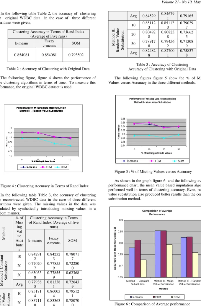
In the following table Table 2, the accuracy of clustering with original WDBC data in the case of three different algorithms were given.
Clustering Accuracy in Terms of Rand Index (Average of Five runs)
k-means Fuzzy
c-means SOM
0.854081 0.854081 0.793502
Table 2 : Accuracy of Clustering with Original Data
The following figure, figure 4 shows the performance of three clustering algorithms in terms of time. To measure this performance, the original WDBC dataset is used.
Figure 4 : Clustering Accuracy in Terms of Rand Index
In the following table Table 3, the accuracy of clustering with reconstructed WDBC data in the case of three different algorithms were given. The missing values in the data was simulated by synthetically introducing missing values in a random manner, M eth o d % of Miss ing Val ue Attri bute s
Clustering Accuracy in Terms of Rand Index (Average of five
runs) k-means Fuzzy c-means SOM M eth o d I Co n sta n t S u b stit u ti o n 10 0.84291 2 0.84232 3 0.78071 7 20 0.77020 7 0.77855 9 0.72280 0 30 0.65033 8 0.77855 9 0.62368 1 Avg 0.77938 5 0.81338 1 0.72643 9 M eth o d II M ea n Va lu e S u b stit u ti o n 10 0.85171 4 0.86003 4 0.79512 1 20 0.83711 0 0.83363 4 0.78070 0 30 0.83825 6 0.83941 4 0.79727 7 Avg 0.84529 0.84679 1 0.79165 M eth o d III Ra n d o m Va lu e S u b stit u ti o n 10 0.85112 3 0.85112 3 0.79029 7 20 0.80492 8 0.80823 8 0.73662 5 30 0.78917 8 0.79456 2 0.71308 9 Avg 0.82482 8 0.82700 1 0.75837 8
Table 3 : Accuracy of Clustering Accuracy of Clustering with Original Data
The following figures figure 5 show the % of Missing Values versus Accuracy in the three different methods.
Performance of Missing Data Reconstruction Method II - Mean Value Substitution
0.74 0.76 0.78 0.8 0.82 0.84 0.86 0.88 0 10 20 30
% of Missing Attribute Values
R a n d I n d e x k-means FCM SOM
Figure 5 : % of Missing Values versus Accuracy
As shown in the graph figure 6 and the following average performance chart, the mean value based imputation algorithm performed well in terms of clustering accuracy. Even, random value substitution also produced better results than the constant substitution method. Comparision of Average Performance 0.65 0.7 0.75 0.8 0.85 0.9 Method I - Constant Substitution Method II - Mean Value Substitution
Method III - Random Value Substitution Method A c c u ra c y w it h R e c o n s tr u c te d D a ta k-means FCM SOM
4.
CONCLUSION
AND
SCOPE
FOR
FURTHER
ENHANCEMENTS
In this paper, we have evaluated three simple missing value imputation algorithms. The performance of the three missing value imputation algorithms were measured with respect to different percentage of missing values in the data set. The perforce of reconstruction was compared with the original WDBC data set.
Among the three evaluated methods, the attribute mean based missing value imputation method reconstructed the missing values in a better manner. Even the random value substitution method also produced more comparable results. The constant substitution method produced poor results compared to the other two methods considered.
For clustering, three different clustering algorithms were used. Among the three clustering algorithms, without missing data, k-means and fuzzy c-means algorithm performed equally and produced good Rand index 0.85. With reconstructed missing data, k-means and fuzzy c-means algorithm were almost performed equally when the percentage of missing values is lower. And if the percentage of missing values is increasing, then FCM seems to be producing little bit better results than k-means in terms of clustering accuracy. But in all the cases, the SOM based clustering algorithm consumed very much time and also produced poor results while comparing it with the other two.
5.
ACKNOWLEDGEMENT
The authors wish to thank the Management and Principal of Sri Ramakrishna Engineering College, Coimbatore – 641 022 for providing resources and support for pursuing research.
6.
REFERENCES
[1] Thomas Lumley, "Missing data", A Lecture Note, BIOST 570, 2005-11-9
[2] Zhang, S.C., et al., (2004). Information Enhancement for Data Mining. IEEE Intelligent Systems, 2004, Vol. 19(2): 12-13.
[3] Qin, Y.S., et al. (2007). Semi-parametric Optimization for Missing Data Imputation. Applied Intelligence, 2007, 27(1): 79-88.
[4] Zhang, C.Q., et al., (2007). An Imputation Method for Missing Values. PAKDD, LNAI, 4426, 2007: 1080-1087. [5] Quinlan, J.R. (1993). C4.5 : Programs for Machine
Learning. Morgan Kaufmann, San Mateo, USA, 1993. [6] Han, J., and Kamber, M., (2006). Data Mining:
Concepts and Techniques . Morgan Kaufmann Publishers, 2006, 2nd edition.
[7] Chen, J., and Shao, J., (2001). Jackknife variance estimation for nearest-neighbor imputation. J. Amer. Statist. Assoc. 2001, Vol.96: 260-269.
[8] Lall, U., and Sharma, A., (1996). A nearest-neighbor bootstrap for resampling hydrologic time series. Water Resource. Res. 2001, Vol.32: 679-693.
[9] Chen, S.M., and Chen, H.H., (2000). Estimating null values in the distributed relational databases environments. Cybernetics and Systems: An International Journal. 2000, Vol.31: 851-871.
[10]Chen, S.M ., and Huang, C.M ., (2003). Generating weighted fuzzy rules from relational database systems for
estimating null values using genetic algorithms. IEEE Transactions on Fuzzy Systems. 2003, Vol.11: 495-506. [11]Magnani, M., (2004). Techniques for dealing with
missing data in knowledge discovery tasks. Available from
http://magnanim.web.cs.unibo.it/data/pdf/missingdata.pdf, Version of June 2004.
[12]Kahl, F., et al., (2001). Minimal Projective Reconstruction Including Missing Data. IEEE Trans. Pattern Anal. Mach. Intell., 2001, Vol. 23(4): 418-424. [13]Gessert , G., (1991). Handling Missing Data by Using
Stored Truth Values. SIGMOD Record, 2001, Vol. 20(3): 30-42.
[14]Pesonen, E., et al., (1998). Treatment of missing data values in a neural network based decision support system for acute abdominal pain. Artificial Intelligence in Medicine,1998, Vol. 13(3): 139-146.
[15]Ramoni, M. and Sebastiani, P. (2001). Robust Learning with Missing Data. Machine Learning, 2001, Vol. 45(2): 147-170.
[16]Pawlak, M., (1993). Kernel classification rules from missing data. IEEE Transactions on Information Theory, 39(3): 979-988.
[17]Forgy , E., (1965). Cluster analysis of multivariate data: Efficiency vs. interpretability of classifications. Biometrics , 1965, Vol. 21: 768
[18]Blake, C.L and Merz, C.J (1998). UCI Repository of machine learning databases.
[19]Hamerly, H., and Elkan, C., (2003). Learning the k in k-means. Proc. of the 17th intl. Conf. of Neural Information Processing System.
[20]Zhang, S.C., et al., (2006). Optimized Parameters for Missing Data Imputation.PRICAI06, 2006: 1010-1016.
[21]Wang, Q., and Rao, J., (2002a). Empirical likelihood-based inference in linear models with mis sing data. Scand. J. Statist., 2002, Vol. 29 : 563-576.
[22]Wang, Q. and Rao, J. N. K. (2002b). Empirical likelihood-based inference under imputation for mis sing response data. Ann. Statist., 30: 896-924.
[23]Silverman, B., (1986). Density Estimation for Statistics and Data Analysis . Chapman and Hall, New York. [24]Friedman, J., et al., (1996). Laz y Decision Trees.
Proceedings of the 13th National Conference on Artificial Intelligence, 1996: 717-724.
[25]John, S., and Cristianini, N., (2004). Kernel Methods for Pattern Analysis. Cambridge.
[26]Lakshminarayan, K., et al., (1996). Imputation of Missing Data Using Machine Learning Techniques. KDD-1996: 140-144
[27]http://archive.ics.ici.edu/ml/datasets/Breast+Cancer+Wisc onsin+%28Diagnostic%29