A subspace recursive and selective feature transformation method for classification tasks

(1)

R E S E A R C H

Open Access

A subspace recursive and selective feature

transformation method for classification tasks

Xuan Zhao

*

and Steven Sheng-Uei Guan

*Correspondence: [email protected] Department of Computer Science and Software Engineering, Xi’an Jiaotong-Liverpool University, 111 Ren’ai Road, 215123 Suzhou, China

Abstract

Background: Practitioners and researchers often found the intrinsic representations of high-dimensional problems has much fewer independent variables. However such intrinsic structure may not be easily discovered due to noises and other factors. A supervised transformation scheme RST is proposed to transform features into lower dimensional spaces for classification tasks. The proposed algorithm recursively and selectively transforms the features guided by the output variables.

Results: We compared the classification performance of linear classifier and random forest classifier on the original data sets, data sets being transformed with RST and data sets being transformed by principle component analysis and linear discriminant analysis. On 7 out 8 data sets RST shows superior classification performance with linear classifiers but less ideal with random forest classifiers.

Conclusions: Our test shows the proposed method’s capability to reduce features dimensions in general classification tasks and preserve useful information using linear transformations. Some limitations of this method are also pointed out.

Keywords: Machine learning, Feature transformation, Feature selection, Classification, Subspace learning

Background

In machine learning tasks the intrinsic representations of high-dimensional data may have much fewer independent variables, as suggested by Hastie [1] in hand written recognitions, the motion of objects [2], and array signal processing [3]. Most of methods trying to solve this problem is domain-specific, like in image processing, the learning of representation often relies on the locality and smoothness assumptions [4]. We are interested in a generally applicable transformation method to transform feature into lower dimensions while preserving useful information for classification tasks.

The proposed algorithm reduces the dataset dimensionality by selectively projecting data points on to the decision plane determined by fitted linear discriminative model. The algorithm is able to run recursively to make better projections.

Notation

Bold lower-case letters denote vectors, e.g.v, and capital letters for matrices, e.g.M. A vectorv’sL1 andL2 norm are denoted byvandv2respectively. Theith row andjth

(2)

column of a matrixMare denoted bym(i)andmj, respectively. We usesampleanddata pointinterchangeably to refer to an observation in the data set.

Classification tasks

Given a dataset X ∈ Rm×n (m samples and n features) and its corresponding class y ∈ {c1,. . .,cc}m. The classes arec;yi is sampleX(i)’s ground truth class. Let xbe a row/sample inX,θbe the model parameters.

A classification task is to construct classifier h(θ) : x → yfrom the seen examples

(X,y)such that for an unseen set of examplesX_pred,h(X_pred,θ)will be as close as possible toy_pred. The modelling process involves minimizing the empirical error betweenyand h(X,θ), denoted asEˆ(y,h(X,θ)). To avoidhover-fits(X,y), the complexity ofhis penal-ized in terms of its some kind of norm||h(·)||p. Therefore a classifier can be trained by solving:

argminθEˆy,h(X,θ)+ h(X,θ)p (1)

Support vector machine

Support vector machines (SVM) is a classic classification algorithm. In the case of two-class two-classification task (y ∈ {c1,c2}m), it minimizesEˆ(y,h(X,θ))by attempting to place a hyperplane,f(X) = wX+w0, between data points from classc1andc2. The classifier h(Xpred)returns a vector of positive or negative signs to indicate the labels ofXpred.

h(X)=sign(wX+w0) (2)

The hyperplane, often known as decision plane, is then optimized to maximize it’s min-imal distance to data points fromc1andc2(also known as the margin). Vapnik showed thatEˆ(y,h(X))can be minimized by maximizing the margin [5]. A penalizing termCis used to control the magnitude of the decision plane misplacing a particular samplexi∈X on the other side. The model complexity can be penalized by minimizingw’sL1norm ||w||orL2norm||w||2[6]

argminw,w0 wp

2 w·X+w0=1+C m

1

ξi (3)

In the proposed algorithmware used to indicate the feature’s contribution to a discrim-inative model. Sincewdefines the direction of the hyperplane separating two classes of data points in thendimensional space, awi ∈ w(i = 1,. . .,n) closing to zero indicates the plane is nearly orthogonal to theithaxis. This intuition has been used in Recursive Feature Elimination [7] method. Figure 1 is a plot of such weights .

Recursive feature elimination

Recursive Feature Elimination (RFE) is a supervised feature ranking and selection tech-nique. It use a classifier’s feature-related weights as the feature importance metrics, such win SVMs or the coefficients in Fischer’s linear discriminator [7, 8].

(3)

Fig. 1Weights from the first label offacesdata set Darker color indicates higher importance. Positive importances is the magnitude of feature’s contribution in classifying this label against the rest, negative is for the rest against this label

Principle component analysis

Principle Component Analysis (PCA) is a feature transformation method that finds a sets of orthogonal components that explain the maximum variance out of the samples. It can also be used to reduce dimensionality of the samples by projecting them to a lower dimensional space (principle component) [9].

PCA algorithm starts with subtracting the mean ofX for all xi ∈ X. Then it com-putes a covariance matrix Cov(_mX,X) by singular value decomposition. Afterwards it finds the eigenvectors withk(k < m)greatest eigen value as the orthogonal components. For a transformation matrixAof sizem×kusingkeigenvectors. The projection ofXto a k-dimensional space isXA.

Feature extraction with SVM

Tajiri et al. proposed a method based for feature extraction using the weight coefficients of a learnt linear SVM classifier for binary classification problems [10]. The intuition is that assume the decision boundary of a linear SVM perfectly discriminates both classes, then the orthogonal hyper plane of the decision boundary, which is determined by the weight coefficients, is an ideal projection plane for the data points to be projected on to embed the discriminative information into the transformed data points.

Recursive Selective Feature Transformation (RST) for classification tasks Feature importance

wfrom the linear SVM model can be seen as how much contribution does each of feature make to form the decision plane.

(4)

Ifwi= −1 or 1, the axis of dimensioniis then orthogonal to the decision plane, which indicates the only by featureican the decision plane discriminate the samples. In most caseswidoes not reach−1 and 1.

Feature importance vectorv

In a binary classification setting where|c| =2, our feature importance vectorv ∈[0, 1]n takes the absolute values of weight vectorw∈[−1, 1]n.

In a multi-class setting|c|>2, ak-class classification problem is solved by One-versus-Rest [11] scheme, which is an ensemble ofk classifiers with each of them trained by discriminating training data fromci∈cagainst the rest (c/ci). In akclass setting there are kws, denoted asW ∈[−1, 1]k×nfrom all sub classifiers in the ensemble, thenvis taken as the mean vector of absolute values ofW.

v= ⎧ ⎨ ⎩

abs(w), if|c| =2 1

k

1abs(W(i)), if|c| =k>2

(4)

Recursive Selective Feature Transformation (RST)

Consider the hypothetical datasetXhasmrows of examples andncolumns of features. We adopted an improved version of the SVM feature extraction method by Tajiri et al. [10]. In short, Tajiri, et al.’s method projects data points on the linear decision plane’s orthogonal plane. Naturally projecting the data points to a hyper-plane in the feature space reduces dimensionality by 1, in other words the projected data points have dimen-sionality ofn−1, thus this approach maintains data points’ inter-class separation while reduces dimensionality.

Therefore reducing the dimensionality to a much smaller number, say k, requires data points being projected n− k times, which involves training SVM model n − k times. Since the approximated time complexity of training a linear SVM model is O(max(m,n)min(m,n)2) [12], assume data sets normally have much more rows than columns, that ism>>n, the time complexity of Tajiri, et al.’s method in this scenario is aroundO(m(n−k)n2), which is expensive to compute for high dimensional data.

To speed up the dimensionality reduction process, RST uses SVM’s weight vector to selected top-k importantfeatures from thefeature importance vector(Eq. 4) to reduce the weight vector to lengthk, and project data points onto ak-dimensional feature subspace determined by the reduced weight vector. Thuskcan be used as a parameter to determine the desired dimensionality. (RST Step 1)

Projecting data points using weights corresponding to thoseless importantfeatures is not ideal since these features contributed less to form current decision plane. They may represent redundant or other non-informative information and therefore can normally be discarded as seen in RFE. A linear decision plane may not generalise on those less important features, therefore RST performs dimensionality reduction on these features with RST Step 1. (RST Step 2).

(5)

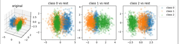
Furthermore, multi-class problem can be difficult for feature extraction based on linear SVM models. The usual approach dealing with multi-class problem is One-versus-Rest (OvR) ensemble [11]. Through this approach, akclass problem leads tokdecision func-tions, i.e.,kweight vectors andkcorresponding intercepts, each of them represents the model for each “one class versus the rest of classes” problems. Obviously averaging the weight vectors, as in the linear models, brings little benefits in terms of generalisation. In RST the i-th(i ∈[ 1,k]) projection matrix is learnt from thei-th weight vectors in the ensemble. Thus upon training a classifier, thei-th sub-classifier in the OvR ensemble learns on data set that has been transformed by thei-th projection matrix, see Fig. 2 for illustration. Upon predicting an unknown sample, RST transforms the sample will be by thekprojection matrices intoktransformed samples for the ensemble to predict.

Methods

Evaluation procedures

The experiments runs for 32 iterations. At each iteration the data set is randomly split with train-test ratio of 3:2. Transformations are learnt by RST, linear discriminant analysis (LDA) [14] and PCA on the training set, then both of the training and testing set are trans-formed with the learnt transformer. RST runs for 6 recursions. Transformation learnt from each recursion were benchmarked. For comparison the number of output features from PCA and LDA is set the same as the number of dimensions of each transformed data set by RST. Due to the nature of LDA, the number of features after dimensionality reduction is strictly less than the number of classes.

The values of data sets has been scaled to [0, 1] without any centering, no missing values or outliers (within +-1.5 IQR) present. Random forest classier and Linear SVM classifier withL2norm penalty and hinge loss is used as the benchmark classifier.

We evaluate the classification performance via multi-class logarithmic loss [15]:

logloss= −1 N

N

i=1 C

c=1

yi,clog(pi,c) (5)

where N is the number of samples being tested, C is the number of classes,logis the natu-ral logarithm,yi,cis 1 if observationiis in classcand 0 otherwise, andpi,cis the predicted probability that sampleiis in classc. This metric takes into account the uncertainty of the classifier’s prediction according to how much it varies from the actual class label. That

(6)

is, lower log loss indicates higher confidence that a classifier makes a correct prediction. Incorrect predictions or uncertain predictions will yield higher log loss.

However naturally linear SVM does not make probabilistic prediction, we obtained it by calibrating our linear SVM model using Niculescu-Mizil’s method [16] via a 3-fold cross-validation.

Data sets

Eight data sets are used to evaluate the proposed method:

1. otto group classification [17] (61878 samples, 93 dimensions, 9 classes) 2. mnist digits recognition [18] (70000 samples, 784 dimensions, 10 classes) 3. olivetti faces recognition [19] (400 samples, 4096 dimensions, 40 classes)

4. sonar: rock vs mine sensory readings [20] (207 samples, 60 dimensions, 2 classes) 5. hand written digits [21] (1797 samples, 64 dimensions, 10 classes)

6. hand written letter recognition [22] (20000 samples, 16 dimensions, 26 classes) 7. glass identification [23] (214 samples, 9 dimensions, 6 classes)

8. iris [24] (150 samples, 4 dimensions, 3 classes)

Results

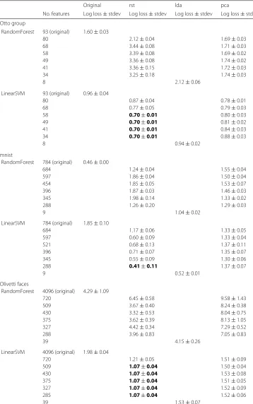
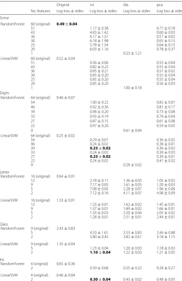
The comparison of Random Forest and SVM performance on original datasets, linear discriminate analysis (LDA) transformed data sets, PCA transformed data sets and RST transformed data sets is in Tables 1 and 2.

Discussion

Among all the transformer (original - no transformation, RST, LDA, PCA) + classifier (Random Forest, Linear SVM) combinations, SVM combined with RST transformation has the best classification performance (lowest logarithmic loss) over all other combi-nations on all the data sets except for sonar andletter. It is noteworthy to mention that none of the transformations improves the classification performance over the origi-nal (un-transformed) data set. While onletterdata set RST+SVM performs better than original+SVM by a small margin but being outperformed by original+RandomForest.

Generally RST works better with linear SVM classifiers than with the non-linear Ran-dom Forest classifiers. With non-linear RanRan-dom Forest Classifier RST, along with other two feature transformers even deteriorates the classification performance. This is not sur-prising since Random Forest’s feature extraction techniques is to use multiple random feature subspaces, i.e. multiple random splits over features; if the set of extracted fea-tures are optimised to be useful and compact, its random subspace is surely a less useful representation.

In most of the cases RST reduces the dimensionality and steadily reduces the log loss at the same time, up to a point where the log loss stops to decrease or starts to increase. Therefore in practice is preferable to add a sub set of data to validate the feature trans-former learnt by RST while training RST so that RST stops learning when not seeing any improvement over log loss.

Conclusion

(7)

Table 1Cross validated (32 runs of 3:2 train-test split) linear SVM and random forest performance on original datasets, RST transformed data sets, LDA transformed data sets and PCA transformed data sets

Original rst lda pca

No. features Log loss_±stdev Log loss_±stdev Log loss_±stdev Log loss_±stdev Otto group

RandomForest 93 (original) 1.60±0.03

80 2.12±0.04 1.69±0.03

68 3.44±0.08 1.71±0.03

58 3.39_±0.08 1.69_±0.02

49 3.36±0.08 1.74±0.02

41 3.36±0.15 1.72±0.03

34 3.25±0.18 1.74±0.03

8 2.12_±0.06

LinearSVM 93 (original) 0.96_±0.04

80 0.87±0.04 0.78±0.01

68 0.77±0.05 0.79±0.03

58 0.70±0.01 0.80±0.03

49 0.70_±0.01 0.81_±0.02

41 0.70±0.01 0.84±0.03

34 0.70±0.01 0.88±0.03

8 0.94±0.02

mnist

684 1.24±0.04 1.55±0.04

597 1.86±0.04 1.50±0.04

454 1.85_±0.05 1.53_±0.07

396 1.87_±0.03 1.46_±0.03

345 1.98±0.14 1.33±0.02

288 1.26±0.20 1.29±0.03

9 1.04±0.02

LinearSVM 784 (original) 1.85±0.10

684 1.17±0.06 1.33±0.05

597 0.60_±0.09 1.33_±0.04

521 0.68±0.13 1.37±0.11

396 0.71±0.07 1.35±0.07

345 0.55±0.09 1.30±0.06

288 0.41_±0.11 1.37_±0.07

9 0.52±0.01

Olivetti faces

RandomForest 4096 (original) 4.29_±1.09

720 6.45±0.58 9.58±1.43

509 3.67±0.40 8.24±0.38

430 3.32±0.53 8.04±0.75

375 3.62_±0.39 8.13_±1.05

327 4.42±0.34 7.29±0.52

288 3.96±0.83 7.05±0.83

39 4.15±0.26

720 1.21±0.05 1.51±0.09

509 1.07_±0.04 1.50_±0.04

430 1.07±0.04 1.53±0.08

375 1.07±0.04 1.51±0.05

327 1.07±0.04 1.52±0.09

285 1.07_±0.04 1.52_±0.06

39 1.53±0.07

(8)

Table 2Cross validated (32 runs of 3:2 train-test split) linear SVM and random forest performance on original datasets, RST transformed data sets, LDA transformed data sets and PCA transformed data sets

Original rst lda pca

No. features Log loss_±stdev Log loss_±stdev Log loss_±stdev Log loss_±stdev Sonar

RandomForest 60 (original) 0.49_±0.04

51 1.17±0.38 0.77±0.18

43 4.83±1.42 0.60±0.03

36 6.17±1.31 0.57±0.02

30 6.18_±1.98 0.65_±0.15

25 5.78±1.54 0.64±0.15

20 6.03±1.16 0.78±0.37

1 9.23±1.21

51 0.56±0.06 0.55±0.04

43 0.82±0.22 0.55±0.04

36 0.85±0.21 0.57±0.02

30 0.85_±0.20 0.55_±0.04

25 0.85±0.20 0.55±0.04

20 0.85±0.20 0.56±0.03

1 1.00±0.18

Digits

54 1.00±0.22 0.82±0.07

46 0.92±0.36 0.81±0.17

39 0.98_±0.20 0.73_±0.08

33 0.93±0.19 0.74±0.04

27 0.87±0.15 0.61±0.08

22 0.97±0.20 0.59±0.05

9 0.61_±0.04

54 0.29±0.01 0.36±0.02

46 0.24±0.02 0.38±0.01

39 0.23_±0.02 0.36_±0.03

33 0.24_±0.02 0.39_±0.03

27 0.23±0.02 0.39±0.01

22 0.24±0.02 0.41±0.02

9 0.28±0.02

Letter

12 2.78±0.11 1.36±0.05 1.05±0.02

9 7.17±0.05 1.61±0.05 1.20±0.03

5 7.08_±0.05 2.28_±0.07 1.96_±0.06

2 7.12±0.16 4.11±0.07 4.98±0.09

12 1.33±0.01 1.62±0.02 1.45±0.01

9 1.37_±0.01 1.89_±0.02 1.66_±0.01

5 1.33±0.03 2.20±0.04 2.05±0.02

2 1.28±0.01 2.51±0.01 2.44±0.01

Glass

RandomForest 9 (original) 2.43_±0.83

5 4.33±1.61 3.53±0.83 2.44±0.88

2 5.80±0.45 3.82±0.61 3.18±1.15

5 1.23_±0.04 1.20_±0.03 1.18_±0.03

2 1.10±0.04 1.22±0.03 1.21±0.05

Iris

2 0.39_±0.68 0.25_±0.22 0.28_±0.27

2 0.30±0.04 0.43±0.02 0.48±0.05

(9)

experiments. However it is performance is not up to the state-of-art. For instance, in Otto Group Classification Challenge data set [17], our result is only comparable to the results from the second quartile, which is typically from gradient boosted tree models with feature engineering.

It is noteworthy to mention that three major limitations of RST needs further improvement. Firstly, the process of feature selection via SVM weights is not a smooth process, thus optimising RST via efficient numeric methods, for instances, stochas-tic gradient descent, is infeasible. Secondly, RST algorithm essentially stacks multiple linear transformations. Although fitting data with linear models are fast and effi-cient, stacked linear transformations are still not capable enough capture the non-linearity in the feature space. Thirdly, RST embeds discriminative information into the input space (feature space) from the output space (class labels). If some outputs (classes) are similar [25] or some samples are mislabelled, RST will make less ideal transformations.

Abbreviations

LDA: Linear discriminate analysis; RFE: Recursive feature elimination; RST: Recursive selective feature transformation; SVM: Support vector machine; PCA: Principle component analysis

Acknowledgments Not applicable.

Funding

This research is supported by Jiangsu Provincial Science and Technology under Grant No. BK20131182, China.

Availability of data and materials

All the data are available from online open data repositories:

1. iris[24]

https://archive.ics.uci.edu/ml/datasets/iris 2. hand written letter recognition[22]

https://archive.ics.uci.edu/ml/datasets/letter+recognition 3. glass identification[23]

https://archive.ics.uci.edu/ml/datasets/glass+identification 4. sonar: rock vs mine sensory readings[20]

http://archive.ics.uci.edu/ml/datasets/connectionist+bench+(sonar,+mines+vs.+rocks) 5. hand written digits[21]

http://scikit-learn.org/stable/modules/generated/sklearn.datasets.load_digits.html 6. mnist digits recognition[18]

http://yann.lecun.com/exdb/mnist/ 7. olivetti faces recognition[19]

http://www.cl.cam.ac.uk/research/dtg/attarchive/facedatabase.html 8. Otto Group Product Classification Challenge[17]

https://www.kaggle.com/c/otto-group-product-classification-challenge/data

Authors’ contributions

Conception and design of study: XZ, SS-UG. Experiment: XZ. Drafting the manuscript: XZ. Revising the manuscript critically for important intellectual content: Xuan Zhao, Steven Sheng-Uei Guan. Both authors read and approved the final manuscript.

Ethics approval and consent to participate Not applicable.

Consent for publication Not applicable.

Competing interests

The authors declare that they have no competing interests.

Publisher’s Note

Springer Nature remains neutral with regard to jurisdictional claims in published maps and institutional affiliations.

(10)

References

1. Hastie T, Simard PY. Metrics and models for handwritten character recognition. Stat Sci. 1998;13(1):54–65. doi:10.1214/ss/1028905973.

2. Tomasi C, Kanade T. Shape and motion from image streams under orthography: a factorization method. Int J Comput Vis. 1992;9(2):137–54.

3. Markovsky I. Low Rank Approximation London: Springer London; 2012. doi:10.1007/978-1-4471-2227-2. http://link. springer.com/10.1007/978-1-4471-2227-2.

4. Bengio Y, Courville A, Vincent P. Representation learning: A review and new perspectives. IEEE Trans Pattern Anal Mach Intell. 2013;35(8):1798–828.

5. Vapnik VN, Vol. 1. Statistical Learning Theory. 1998.

6. Weston J, Elisseeff A, Schölkopf B, Tipping M. Use of the zero-norm with linear models and kernel methods. J Mach Learn Res. 2003;3:1439–61.

7. Gysels E, Renevey P, Celka P. Svm-based recursive feature elimination to compare phase synchronization computed from broadband and narrowband eeg signals in brain–computer interfaces. Signal Process. 2005;85(11):2178–89. 8. Louw N, Steel S. Variable selection in kernel fisher discriminant analysis by means of recursive feature elimination.

Comput Stat Data Anal. 2006;51(3):2043–55.

9. Jolliffe I. Principal Component Analysis. New York: Springer-Verlag; 2002.

10. Tajiri Y, Yabuwaki R, Kitamura T, Abe S. Feature Extraction Using Support Vector Machines Vol 6444, LNCS. 2010. p. 108–15.

11. Rocha A, Goldenstein SK. Multiclass from binary: Expanding one-versus-all, one-versus-one and ecoc-based approaches. IEEE Trans. Neural Netw Learn Syst. 2014;25(2):289–302.

12. Chapelle O. Training a Support Vector Machine in the Primal. Neural Computation. 2007;19(5):1155–78. doi:10.1162/neco.2007.19.5.1155. http://www.mitpressjournals.org/doi/10.1162/neco.2007.19.5.1155.

13. Fan RE, Chang KW, Hsieh CJ, Wang XR, Lin CJ. LIBLINEAR: A Library for Large Linear Classification. J Mach Learn Res. 2008;9(2008):1871–4. doi:10.1038/oby.2011.351.

14. Yu H, Yang J. A direct LDA algorithm for high-dimensional data – with application to face recognition. Pattern Recogn. 2001;34(10):2067–70. doi:10.1016/S0031-3203(00)00162-X.

15. Rosasco L, Vito ED, Caponnetto A, Piana M, Verri A. Are Loss Functions All the Same? Neural Comput. 2004;16(5): 1063–76. doi:10.1162/089976604773135104.

16. Niculescu-Mizil A, Caruana R. Predicting good probabilities with supervised learning. In: Proceedings of the 22Nd International Conference on Machine Learning. ICML ’05. New York: ACM Press; 2005. p. 625–32.

doi:10.1145/1102351.1102430. http://doi.acm.org/10.1145/1102351.1102430.

17. Kaggle. Otto Group Product Classification Challenge. 2015. https://www.kaggle.com/c/otto-group-product-classification-challenge/data. Accessed 05 June 2017.

18. LeCun Y, Cortes C, Burges CJC. Mnist handwritten digit database. AT&T Labs. 2010;2. [Online]. Available: http://yann. lecun.com/exdb/mnist.

19. Ahonen T, Hadid A, Pietikäinen M. Face recognition with local binary patterns. Computer vision-eccv 2004. 2004;469–481. doi:10.1007/978-3-540-24670-1_36. http://link.springer.com/10.1007/978-3-540-24670-1_36. 20. Gorman RP, Sejnowski TJ. Analysis of hidden units in a layered network trained to classify sonar targets. Neural

Netw. 1988;1(1):75–89.

21. Denker JS, Gardner W, Graf HP, Henderson D, Howard R, Hubbard WE, Jackel LD, Baird HS, Guyon I. Neural network recognizer for hand-written zip code digits. In: NIPS. 1988. p. 323–31.

22. Frey PW, Slate DJ. Letter recognition using holland-style adaptive classifiers. Mach Learn. 1991;6(2):161–82. 23. Evett IW, Spiehler EJ. Rule induction in forensic science. In: Knowledge based systems. Halsted Press; 1988. p.

152–60. http://www.cs.ucl.ac.uk/staff/W.Langdon/ftp/papers/evett_1987_rifs.pdf.

24. Hertz Ja, Krogh AS, Palmer RG, Weigend AS. Introduction to the Theory of Neural Computation. Artificial Intelligence. 1993;I(June):1–17.

25. Zhao X, Guan S, Man KL. An Output Grouping Based Approach to Multiclass Classification Using Support Vector Machines. In: Advanced Multimedia and Ubiquitous Engineering. 2016;389–395. doi:10.1007/978-981-10-1536-6_51. http://link.springer.com/10.1007/978-981-10-1536-6_51.

• We accept pre-submission inquiries

• Our selector tool helps you to find the most relevant journal

• We provide round the clock customer support

• Convenient online submission

• Thorough peer review

• Inclusion in PubMed and all major indexing services

• Maximum visibility for your research

Submit your manuscript at www.biomedcentral.com/submit