Study of sluice gate flow using the finite element method.

(1)

University of Windsor University of Windsor

Scholarship at UWindsor

Electronic Theses and Dissertations Theses, Dissertations, and Major Papers

3-1-1970

Study of sluice gate flow using the finite element method.

C. Y. Li

University of Windsor

Follow this and additional works at: https://scholar.uwindsor.ca/etd

Recommended Citation Recommended Citation

Li, C. Y., "Study of sluice gate flow using the finite element method." (1970). Electronic Theses and Dissertations. 6618.

https://scholar.uwindsor.ca/etd/6618

This online database contains the full-text of PhD dissertations and Masters’ theses of University of Windsor students from 1954 forward. These documents are made available for personal study and research purposes only, in accordance with the Canadian Copyright Act and the Creative Commons license—CC BY-NC-ND (Attribution, Non-Commercial, No Derivative Works). Under this license, works must always be attributed to the copyright holder (original author), cannot be used for any commercial purposes, and may not be altered. Any other use would require the permission of the copyright holder. Students may inquire about withdrawing their dissertation and/or thesis from this database. For additional inquiries, please contact the repository administrator via email

(2)

INFORMATION TO USERS

This manuscript has been reproduced from the microfilm master. UMI films

the text directly from the original or copy submitted. Thus, some thesis and

dissertation copies are in typewriter face, while others may be from any type of

computer printer.

The quality of this reproduction is dependent upon the quality of the

copy submitted. Broken or indistinct print, colored or poor quality illustrations

and photographs, print bleedthrough, substandard margins, and improper

alignment can adversely affect reproduction.

In the unlikely event that the author did not send UMI a complete manuscript

and there are missing pages, these will be noted. Also, if unauthorized

copyright material had to be removed, a note will indicate the deletion.

Oversize materials (e.g., maps, drawings, charts) are reproduced by

sectioning the original, beginning at the upper left-hand corner and continuing

from left to right in equal sections with small overlaps.

ProQuest Information and Learning

300 North Zeeb Road, Ann Arbor, Ml 48106-1346 USA 800-521-0600

(3)

(4)

STUDY OF SLUICE GATE FLOW USING

THE FINITE ELEMENT METHOD

A Thesis

submitted to the F a c u l t y of Graduate Studies

in partial fulfilment of the requirements

for the degree of

Master of Applied Science

in the Department of Civil Engineering

University of Windsor

by

C. Y. Li, B.Sc.E,

Windsor, Ontario

March, 1970

(5)

UMI Number: EC52812

d>

UMI

UMI Microform EC52812

unauthorized copying under Title 17, United States Code.

ProQuest Information and Learning Company 789 East Eisenhower Parkway

P.O. Box 1346 Ann Arbor, Ml 48106-1346

(6)

APPROVED BY

(7)

AC KNOWLEDGEMENTS

The author ivishes to express his sincere thanks to

Prof. J.A. McCorquodale for patient guidance offered

throughout this work, and to Dr. S.P. Chee for helpful

advices during this study. The author also wishes to say

his thanks to Mr. H. NG, Mr. P. Feimer and Mr. G. Michalczuk.

The author is grateful to Dr. J.F. Leddy, President,

University of Windsor and the National Research Council for

the financial support given.

(8)

ABSTRACT

This paper presents the results of a numerical analysis

and an experimental study of the irrotational gravity affected

flow under sluice gates.

A finite element procedure is presented for the numerical

analysis part of the study. The contraction coefficient,

discharge coefficient and downstream water surface profile

are the main parameters obtained. The flow field is discretized

by triangular elements and the ouflow free surface is

represented, by a portion of an ellipse. The downstream free

surface profile is satisfied by choosing the major and minor

axes of the ellipse, that minimize the deviation from the

constant energy requirement. An iterative successive

overrelaxation procedure was used to solve the unknown nodal

values of the stream function.

Vertical gates with 0.47 inches thickness for 0°, 15°» 30°

gate lips were used for the numerical analysis and experimental

study. Vertical gates with 2.0 inches thickness for 15

°,

30°,

45° gate lips were also used f o r .experimental study.

It was found that the computer results compare

satisfactorily with analytical and experimental data.

(9)

i i i

CONTENTS

Page

List of tables v

List of figures vii

List of photographs xi

Nomenclature xii

1 Introduction 1

2 Survey of literature 3

3 Theoretical study 10

3.1 Basic idea of finite element method 10

3.2 Two-dimensional formulation 11

3.3 Slope matrix

14-4- Application of finite element method to the

sluice gate 15

5 Experimental equipment 26

5.1 Facilities 26

5.1.1 Flume set up 26

5 . 1 .h sluxce gate set up 2c

5.1.3 Auxiliary equipments 29

5.2 Experimental procedures 35

5.2.1 Downstream water surface profile

measurement 35

5.2.2 The measurement of coefficient of

contraction 35

6 Numerical results 38

6.1 Computed coefficients of contraction 38

6.2 Computed coefficients of discharge 39

6.3 Contour map 4-0

6.4- Downstream free surface profile 4-0

7 Experimental results 55

7.1 Downstream free surface profile measurement 55

7.2 Measurement of coefficients of contraction 55

7.3 Coefficient of discharge 57

(10)

iv

Page

8 Discussion

104-8.1 The choice of elements

104-8.2 Comparison of energy method and momentum

method 106

8.3 The difference between experimental results

and computed results 106

8.4- Comparison of different theoretical

solutions 108

8.5 Contour map. 108

8 . 6 The accuracy of experimental readings 109

8 . 7 The accuracy of results 111

9 Conclusion 123

Reference 125

Appendix 1 128

Appendix 2 135

Vita auctoris 14-9

(11)

LIST OF TABLE

Table Page

2 . 1 Coefficients of contraction by Benjamin 6 6 . 1 Some parameters used in the numerical solution 38

6 . 2 Computed

CQ

and by energy principle 41

6.3 Computed C and C-p by momentum principle 42

7.1 Experimental downstream free

for sharp edged g a t e (1=24")

surface profile

58

for sharp edged gate(D=1 5")'

surface profile

59

for sharp edged gate(D=7.5")

surface profile

60

for 15° bevelled g a te(B=24")

surf ac e profile

61

for 15° bevelled gate(D=1 5")

surface profile

62

7.6 Experimenatl downstream free surface profile

for 15” bevelled gate(D=7.5" ) 63

for 30° bevelled gate(D=24")

64

for 30° bevelled gate(D=1 5")

65

7.9 Experimental downstream free surface profile

for 30_{° bevelled gate(D=7.5" )} 66

7 . 1 0 Experimental downstream free surface profile

for 15° bevelled g a t e (3=24", t =2.0") 67

7.11 Experimental downstream free surface profile

for 15° bevelled gate(D=15'Vt=2.0") 68

7 . 1 2 Experimental downstream free surface profile

for 15° bevelled vgate(D=7.5" ,t =2.0") 69

7.13 Experimental downstream free surface profile

for 30° bevelled gate(D=24",-o=2.0") 70

(12)

vi

Table Page

7.14 Experimental downstream free surface

for 30° bevelled g a t e ( D =1 5‘’ ,t=2.0" )

profile

71

7.15 Experimental dov/nstream free surface

for 3 0° bevelled g a t e ^ D ^ * 5”

• >

t =2.0" )

profile

72

for 45° bevelled gate(D=24",t=2.0")

profile

73

7-17 Experimental downstream free surface

for 45° bevelled gate(D=15",t=2.0")

profile

74

for 45° bevelled gate(D=7.5 "1t = 2 . 0 " )

profile

75

7.19 Experimental

CQ

and for sharp edged gate 76

7 . 2 0 Experimental C and C-r. for 30° bevelled gate 77

7 . 2 1 Experimental

GQ

and for 15 bevelled gate 78

7 . 2 2 Experimental C and for 30° bevelled gate

Ct=2.0") 79

7.23 Experimental C and for 15° bevelled gate

(t=2.0") 80

7.24 Experimental Cc and for 45° bevelled gate

(t=2.0") 81

7.25 Experimental Cc and for sharp edged gate

(G=6.016") 82

7.26 Experimental Cc and for sharp edged gate

(G = 1 .023") 83

8.1 Eo. of elements along u pstream side of the gate 105

8.2 Percentage error of C 114

8 . 3 The scatter of experimental results 115

(13)

v i i

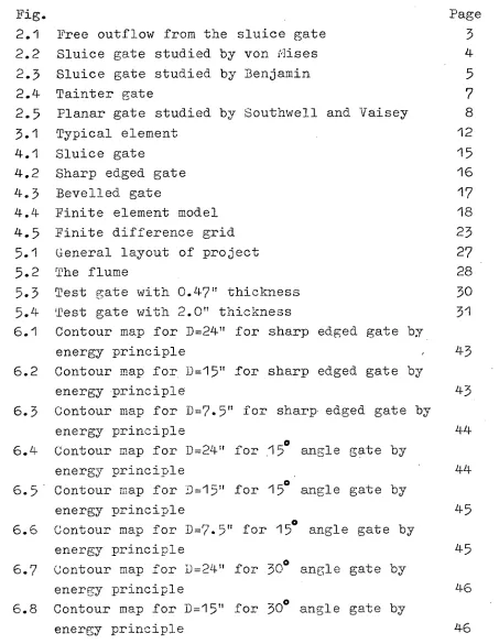
LIST OP-FIGURES

Fig.

Page

2.1 Free outflow from the sluice gate 3

2.2 Sluice gate studied by von Mises 4

2.3 Sluice gate studied by Benjamin 5

2.4 Tainter gate 7

2.5 Planar gate studied by Southwell and Vaisey 8

3.1 Typical element 12

4.1 Sluice gate 15

4.2 Sharp edged gate 16

4.3 Bevelled gate 17

4.4 Finite element model 18

4 . 5 Finite difference grid 23

5.1 General layout of project 27

5.2 The flume 28

5.3 Test gate with 0.47" thickness 30

5.4 Test gate with 2.0" thickness 3i

6.1 Contour map for D=24" for sharp edged gate by

energy principle , 43

6.2 Contour map for D=15" for sharp edged gate by

energy principle 43

6.3 Contour map for D=7.5" for sharp- edged gate by

O

6.4 Contour map for 0=24" for .15 angle gate by

_ o

6.5 Contour map for 0 = 13" for 15 angle gate by

O

6 . 6 Contour map for 0=7.5" for 15 angle gate by

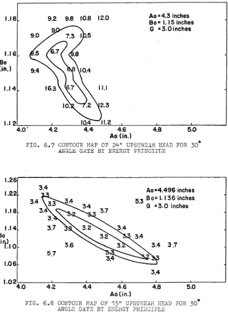
6.7 Contour map for 0=24" for 30° angle gate by

6 . 8 Contour map for D=15" for 30° angle gate by

(14)

viii

Fig. 6.9

6.10

6.11

6.12

6.13

6.14 6.15 6.16 6.17 6.18 6.19

6.20

6.21

7.1 7.2 O

Contour map for D=7.5" for 30 angle gate by

energy principle

Contour map for D=24" for sharp edged gate by

momentum principle

Contour map for D=15" for sharp edged gate by

Contour map for 0=7.5" for sharp edged gate by

O

Contour map for D=24" for 15 angle gate by

O

Contour map for 0=15" for 15 angle gate by

O

Contour map for D=7.5" for 15 angle gate by

o

Contour map for 0=24-" for 30 angle gate by

Contour map for 0=15" for 30° angle gate by

Contour map for 0=7.5" for 30° angle gate by

Theoretical coefficients of discharge for sharp

edged gate

O Theoretical coefficients of discharge for 30

angle gate

Theoretical coefficients of discharge for 15°

angle gate

Experimental coefficients of contraction for

sharp edged gate(G=6.016")

Experimental coefficients of contraction for

sharp edged gate(G=3.016")

Page

4-7 4-8 4-8 4-9 4-9 50 50 51 51 52 53 54-55 84 85

(15)

ix

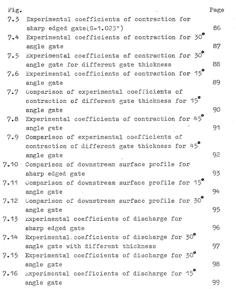
Fig.

Page

7-3 Experimental coefficients of contraction for

sharp edged g a t e (.G = 1 .023" ) 86

o 7.4- Experimental coefficients of contraction for 30

angle gate 87

o 7.5 Experimental coefficients of contraction for 30

angle gate for different gate thickness 88

O 7.6 Experimental coefficients of contraction for 15

angle gate 89

7.7 Comparison of experimental coefficients of

o

contraction of different gate thickness for 15

angle gate 90

°

7.8 Experimental coefficients of contraction for 45

angle gate ' 91

7.9 Comparison of experimental coefficients of

_o contraction of different gate thickness for 45

angle gate 92

7.10 Comparison of downstream surface profile for

sharp edged gate 93

o

7-11 Comparison of downstream surface profile for 15

angle gate 94

O

7.12 Comparison of downstream surface profile for 30

angle gate 95

7.13 Experimental coefficients of discharge for

sharp edged gate 96

7.14 Experimental.coefficients of discharge for 30°

angle gate with different thickness 97

7.15 Experimental coefficients of discharge for 30°

angle gate 98

O

7-16 experimental coefficients of discharge for 15

angle gate 99

(16)

Pig. 7.17 7.18 7.19

7.20

.

8.1

8.2

8.3 8.4 8.5

8.6

8.7 x o Experimental coefficients of discharge for 15

angle gate with different thickness

O Experimental coefficients of discharge, for 45

angle gate

Experimental coefficients of discharge for

sharp edged g a t e (G=6.016")

Experimental coefficients of discharge for

sharp edged g a t e ( G = 1 .023")

Coefficients of contraction for sharp edged gate

for different gate opening 116

Theoretical coefficients of contraction for

sharp edged gate by different methods 117

Comparison of experimental results with

-theoretical results for sharp edged gate 118

Comparison of experimental coefficients of

contraction wi t h theoretical coefficients of

contraction for 3 0° angle gate 119

Comparison of theoretical coefficients of

contraction for 3 0° angle gate 12 0

Comparison of experimental results with

theoretical results for 1 5° angle gate 121

Percentage error of coefficients of discharge 122

Page

100

101

102

103

(17)

LIST OP PHOTOGRAPH

P h o t o . . Page

5.1.a Test gate of 1 5° and 30° ' 32

5.1.b Test gate of 4-5° 33

5.2 Electric point gauge

34-5.3 Magnetic flow meter 35

(18)

NOMENCLATURE

[a ] Coefficient matrix,

a Height of the axis of Tainter gate.

A0 Major axis of ellipse.

B0 Minor axis of ellipse.

CC Downstream water depth where the water

surface is parallel to the floor.

C c Coefficient of contraction.

CD Coefficient of discharge.

D Upstream depth.

E Downstream total energy.

G Gate opening,

g Gravitational acceleration.

H Upstream head on gate.

hQ , h Depth of water infinitely far upstream,

[h] Coefficient matrix,

i, j, k Indices referring to nodes.

P Force on the gate.

Pe Percentage erro of Cp.

'Q Discharge,

q Discharge per unit width.

(19)

X I 11

Radius of Tainter gate

Error summation.

Sj_j Stiffness matrix.

t,t' Gate thickness.

U Upstream w ater velocity.

U Downstream xrater velocity.

|vTj Constant' matrix.

(x, y) Rectangular coordinates.

9 Angle of inner gate force with vertical line.

$ Angle of inner gate force with horizontal line.

A / .A.

Stream function.

A Area o f triangular element.

A . Discrepancy in C c for Gj_.

{ ^ } Stream function corresponding to element.

£ Deviation of energy.

& Boundary layer thickness.

\J Kinematic- viscosity,

k) Over-relaxation factor.

(20)

1

CHAPTER 1

INTRODUCTION

The purpose of this project is the study of gravity

flow under sluice gates? this problem has been investigated

by a number of researchers using methods which will be

described the next chapter. These methods include conform el

mapping, finite differences,, infinite series, complex function

analysis and a combination of conformal mapping and. Riemann.--

Hilbert.

In channels, the d ep th-d.ischarge relationships are

often determined by the control mechanisms operating within

it, There are different kinds of control mechanism, which

can indicate what the depth must be for a given discharge

and vice versa. One of these control mechanisms is the sluice

gate which is discussed here.

Water area at the section downstream from the gate is

contracted due to the presence of the sluice gate. The ratio

of this contracted area at the downstream section, where the

water surface is horizontal, to the water area at the gate

opening is called the coefficient of contraction, Once this

ratio is known, the water area at the downstream section can

be obtained and the discharge of water can be estimated.

The determination of coefficients of contraction for

different types of sluice gate lips is a major part of this

work. Sharp crested gates and gates with 15°» 30° , ^5°

(21)

bevelled lips of 0.5 inch thicknesses are studied

theoretically and experimentally. Also 15° » 30° » !+5° angle

gates with 2.0 inch thicknesses are studied‘experimentally.

The theoretical approach of this work is based on the

finite element method , in which the stream functions and

coordinates at some selected points in the flow are to be

determined. The computer programme for of the finite element method

uses an iterative procedure to determine the final answer to

the desired degree of accuracy. By adjusting the two parameters

Ao and Bo of an ellipse, the downstream surface profile can be

determined. The elliptical equation with the A o , Bo which

gives the minimum deviation can be used to express the downstream

surface profile and vena contracts..

The experimental results were obtained by measuring the

downstream tailwater depth at a sufficient distance downstream

from the gate v?ith an electric point gangs. Bets of readings

are obtained for different flow conditions and different types

of gates.

The experimental and computed results are c o m p a r e d . These

are also compared with the results of previous investigators.

T h e f i n i t s cT^rn^ni" sol i o n s svTH6*s d o vj s c o s i t v dD.T d o

SDD'f'cXCO t O D s ^ o D i n tti0 flul-T « A T so T h e v- o s A n o citt v o T o c i t y

h e a d is c o n s i d e r e d i n t h i s s t u d y . A c o r r e c t i o n o f u p s t r e a m

d e p t h i s m a d e a t t h e b e g i n n i n g o f t h e c o m p u t e r p r o g r a m m e . T h e

coefficients of contraction and the parameters Ao,Bo are printed

‘'out in the computer programme for different heads and different

typos of gate lips.

(22)

3

CHAPTER 2

SURVEY OF LITERATURE

In

1876

, Rayleigh (1) found the solution of the problem

•) from the sluice gate (Pig, 2,1) of free outflow

The dorr.stream free surface satisfied the equation

CC

1 _ s m e

where 9 is the downstream water surface slope tar * (dy/dx),

which ranres between 0 and- jr_

2

>.nd CC is the downstream water

depth where writer surface is horizontal.

In the corresponding .gravity problem, vrhere F is very

large, the equation

CC

1 —

_{tan 0 ,}

_(G<Sd)

_{__ (2.2)}

can be used; thence two equations give nearly the same results.

(23)

4-R. Von Kises (2) dealt with flow under a sluice

;izzz'z;z.z.z./--z:z

CC

X

Fig. 2 . 2

. ’-To assumed that in the region B, the flow is little

,-cted ly gravity,since the acceleration o f . the flow particle:

,ai there, The free surface of Fig, 2,2 was given by the

CC 2D-CC

71 m

-I

V7jh X* 0

2 D'CC

- Iv

in © )

-CC CC TC m

G is the gate opening;

© is the anrular slore of the profile ,,, (2.3)

The first investigator dealing.analytically with a sluice

gate flow under the influence of gravity appears to have been

Pajer (3) in 1937. He assumed an ellipse could be used in the

hodogreph plane in the conforms! mapping method. The fixed

free stream line, and the boundary condition of constant

;r assure were not verified. The resulting line

was correct at the end points, and

(24)

nearly correct at points in between.

In 1946, Southwell and Vaisey (4) assumed the conditions

of Pig. 2.1, where D=12 and h =11 length units, and the CC

calculated from the continuity and Bernoulli equations was

3.854 length unit. The Froude number used was 2.055* They

included the upstream free surface and solved the Laplace

equation for a sluice gate by substituting a finite difference

equation for the partial differential equation and applying

a relaxation procedure. In their ifork, viscosity effects were

not taken into consideration. They found C c= O.6 0 8 for

CC/H = 0.312.

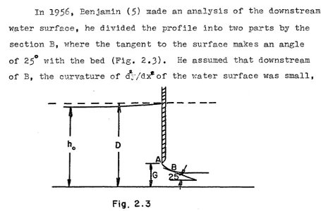
In 1956, Benjamin (5) made an analysis of the downstream

water surface, he divided the profile into tx?o parts by the

section B, where the tangent to the surface makes an angle

of 25° with the bed (Fig. 2.3), He assumed that downstream

of B, the curvature of d2y/dx*of the water surface was small,

Fig. 2,3

and that all higher derivatives of y were of rapidly diminishing

order. In the region A B this assuption is no longer valid.

An approximate solution was found by taking Von M i s e s1

(25)

6

solution for the non-gravity case and superimposing on it an

allowance for the variation of surface velocity between A and 3,

The two solutions were fitted together at the section B, the

results are given in the following table 2,1.

Table 2.1

G

/3

0 0.1 0.2

0.3

0. b

_0.5

rp 0.611 .0 Sp. £ 0,602 0.60

₀

.

59

S

0,598

Perry (6) in 1957 improved the holograph method by an

infinite series method, The pressure can be made constant at .

a finited number of points by including more terms of the infinite

series. In actual application of the mappings he took a finite

number of terms in the series and carry through the complete

calculation to find the vertical coordinate of the free

streamline y in terms of the N arbitrary coefficients b..

In pi’actice the numerical wor k can be reduced somewhat by noting

, and the rest of bn * s are small compared to unity,

Fangmeier and Strelhoff (?) In

1968

, avoided using

holograph plane and- employed complex function theory to evaluate

a nonlinear integral equation for this problem, from which the

solution is deduced. They considered fully both the Influences

of gravity and the upstream free surface, however, their

method, apparently requires extensive computer time.

In the laboratory, sluice gates are usually sharp edged,

because of structure reasons and difficulties of sealing at

(26)

complete closure, this is not always practical for field

conditions,

In 19 3 3 f Mueller(8) made the lip profile elliptical at

the entrance and exit sections.

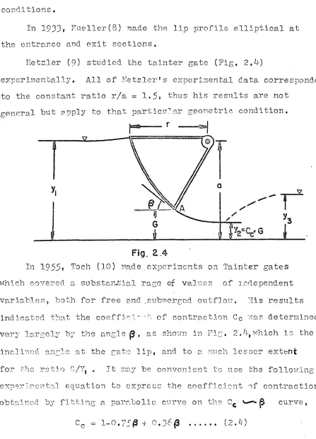
Ketzler (Q) studied the tainter gate (Pig, 2,4)

experimentally. All of Metzler’s experimental data corresponded

to the constant ratio r/a = 1.5* thus his results are not

general but apply to that particular geometric condition.

-SL

1 Fig. E.4

In 1955, Tech (10) m a d e .experiments on Tainter gates

which cornered a su.bstan.tial rage of values of independent

variables, both for free and. .submerged, outflow. His results

indicated, that the coefflei t of contraction C c was determined

very largely by the angle p , as shown in Fig, 2,4, which Is the

inclined angle at the gate lip, and to a much lesser extent

for the ratio 0/Y, . It may be convenient to use the following

experimental equation to express the coefficient of contraction,

obtained by fitting a parabolic curve on. the Cc v— * ft curve,

1-0.75(3 + 0.36(3 (2.4)

(27)

Where the unit of

(3

is taken as 90° • Equation (2.*)-)

gives results which are accurate to

±5%,

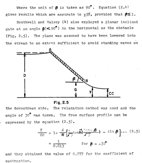
provided that ^ < 1.

Southwell and Vaisey (^) also employed a planar inclined

gate at an angle £(<.90°) to the horizontal as the obstacle

(Fig. 2.5). The plane was assumed to have been lowered into

the stream to an extent sufficient to avoid standing waves on

CC

Fig. 2.5

the downstream side. The relaxation method was used and the

angle of 30° was taken. The free surface profile can be

expressed by the equation (2.5)»

CC

for

p

= - 3 0

0.813

and they obtained the value of

0.777

for the coefficient of

contraction.

In 1969» Larock (11) developed a solution for any arbitrary

gate inclination

p

(0 < 0 < T C ) , in such a way that an extension

to the analytical consideration of curved (radial and Tainter)

gates appears feasible. He combined the conformal mapping and

(28)

Riemann-Hilbert solution to a mixed boundary condition problem

to solve the problem of gravity- affected flow from planar

sluice gates of arbitrary inclination.

(29)

1 0

CHAPTER 3

THEORETICAL STUDY

3.1 Basic Idea of Finite Element Method

According to Zienkiewicz (12), problems of potential

distribution in a continuous medium can be solved by using

the finite element method. The procedure for solution is

summarized as follows:

a) The continuum is isolated by imaginary lines or

surfaces into a number of finite divisions or regions,

b) The elements are assumed to be interconnected at a

discrete number of nodal points situated on their

boundaries. The characteristic values of these nodal

points will be the basic unknown parameters of the

problem.

c) A function is chosen to define uniquely the state of

the dependent variables within each "finite element"

in terms of its nodal values.

d ) The function now defines uniquely the state of potential

within an element in terms of the nodal values. These

potentials together with any initial potentials and

the characteristic properties of the material will

define the state of energy throughout the element and,

hence, also on its boundaries.

e ) A stiffness or geometric relationship is developed

to solve the problem.

(30)

1 1

3.2 Two Dimensional Formulation

t

For irrotational, incompressible flow, the two demensional

formulation to specify the energy function is

where

is the unknown stream function, assumed to

be single valued,

is the energy function.

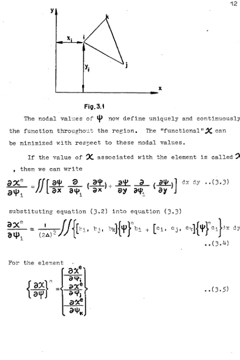
Consider now the region divided into triangular elements.

Let the nodal values of 4^ define the function of dependent

variables within each element. For a typical triangle ijk

(3.D

(Fi

(3.2)

in which

a i= x jy k - y jx k

b i= yj - y k = y jk

Ci= x k - x ji= x k - x j = x kj

1 3Ci y i T_{_L}

2A= det i x j ^j = 2 ( area of triangular ijk)

1 x k y k

(31)

1 2

y

Fig. 3.1

The nodal values of Ip now define uniquely and continuously,

the function throughout the region. The " f u n c t i o n a l " ^ can

be minimized with respect to these nodal values.

If the value of associated with the element is called

, then we can write

a X

a f .

=//[-a t

3 , a t \

/

<sT

v ^

a t

o'r

9 f

q

/ o r

\

ax dy ..(3.3)

**ax aq> v a x ; * ©y**

vay

substituting equation (3-2) into equation (3*3)

d i p- = 7^ / / { [ b 11 b 3 * bk]{l,f b i + [0 1 ' °J- c '0 H ”O i } ax d y

..(3.^)

For the element

e

{

f

T

-a x

a4>;

a x e

a x e

..(3.5)

(32)

13

Therefore

. .

(3*6)

noting again

/ / dx dy = A

this leads to the stiffness matrix,

hi m = M =

_h.A1

V i b k b i"

1 ° i c i c jc i ck c i

b kbj

+ A C.C. i J C • C • 3 3 k 3^ ■?

_bibk b j b k _{b k b k} _{,c i ck} _{c jck} _{ck ck_}

..(3.7)

The final equation of the minimization procedure requires

the assembly of all the differentials o f X and the equating

of these to zero

a x _y a x e ; 0

9 ^ ..(3.8)

The summation in equation (3.9) being taken over all

elements and nodes i.e.

= = o ..(3.9)

where m is a dummy index.

(33)

1 4

3.3 Slope Matrix

In some situations the quantity of interest is the

gradient o f ^ . The two components of the gradient can be

obtained from equation (3.10).

■jgrad l|>

d x

'b i b ^ b kV

< > = — — <

2 A

> <

* 3 >

a y

c i c k

-*■ o V k

..(3.10)

(34)

1 5

CHAPTER

APPLICATION OF FINITE ELEMENT METHOD

TO THE SLUICE GATE

When flow changes from subcritical (V</gjF) to supercritical

(V>/sy) through a controlled section, the Froude number is the

most important governing factor, i,e. this flow is under the

influence of gravity. The downstream flow is said to be free,

if the issuing jet of supercritical flow is open to atmosphere

i.e. it is not submerged by tailwater (Fig. *Kl).

“T

Fig. 4 .1

In this study, the finite element method is used to

solve the problem of flow from sluice gates under the influence

of gravity.

At the downstream water surface, there are two tangent

conditions at points A, 3 on the outflow water surface profile;

one is at the gate lip A and the other is the point B on the

downstream water surface where the depth of water is equal

(35)

1 6

to the tailwater depth and water surface approaches horizontal.

The water surface profile between points A, B is a smooth

curve. In general, the direction of flow at the gate lip

is tangent to the inner surface of the gate lip which may

be

vertical or at an angle. The direction of flow at the other

point, i.e, where the depth of water is equal to tailwater

depth is parallel to the floor. Owing to above characterisics,

it is assumed that the profile can be approximated by part

of an ellipse equation as shown in Fig. 4.2 and Fig. 4.3.

If the gate lip is vertical and sharp-edged, the profile

can be expressed by equation (4.1) and as shown in Fig. 4.2.

If the gate lip is bevelled, the profile can be expressed

by equation (4.2) and as shown :n Fig. 4.3.

(4.1)

D

x

Fig. 4.2

(36)

17

pro f :

prooe

where

p

.

CC = G +

/

'■_{Bo +Ao tan}— ■" ■ ni

p

— - ' O

DD = A02tanj

/

h / i - A ^ t a n ^ 90

-/ / / / / / / / /

vfl Ao !

\

xr - *r --- /■

X D D ^ C C -SawK

Fig. 4.3

The coordinates of the points on the downstream free surface

ile are based on equation 4,1 and equation 4,2, The

:dure for setting up the finite element method is as follows:

(a) Sketches a few streamlines through the region of

interest. Both upstream and downstream boundaries

should be located to make sure that the flow at these

sections nearly parallel flow as shown in Fig. 4,4.

The upstream free surface js first assumed to be

h o r i z o n t a l , and downstream surface is assumed to be

-elliptical based on equation (4.1) ana equation (4.2)

Line ABCG and line FF 3 n F3 p. 4.4 are employed as two

bo undary strcaml3n o s .

(37)

1 8

t=0.47 inches

Ellipse

=Q

H > = 0

OUTFLOW SECTION

TYPICAL ELEMENT

TOTAL ENERGY LINE

GATE PRESSURE

FIG. 4.4 FINITE ELEMENT MODEL

(38)

19

The stream function at the upstream, AP, and

downstream, DE, boundaries are based on the ratio of

the depth to total depth times the total flow.

(b) Several triangular elements are drawn between

adjacent streamlines, all the nodes of the elements

are located on the approximated streamlines,

(c) The coordinates of each node and the approximate

value of stream function

(HO

on each node are

determined. The values of stream function (IfO on

the boundary streamlines are assumed to be known.

(d) Substitute the coordinates and the values of the

nodal stream functions into the equation (3*9)•

= 0

..(3.9)

>

where

"b Ib i b Jb i V Di’ c ic i c jc i o rk o H*

1

b ^

5 ~ j b .b-.J .1 b, b .k .] 1

2 A

c.c. n r»

j'M ck°j

b lb k b kb k ° ic k c jc k c kc k

..(3.7)

If there are N unknown nodes, N simultaneous equations

will be obtained.

(39)

2 0

(e) The extrapolated Liebmann method. (13) »(1*0 also

known as the ’extrapolated Gauss-Seidal1 and

'Successive overrelaxation' method is used, to solve

these linear simulaneous equations (eq. 3*9),

the iterative procedure can be written in the form.

Dnew =U0UL + (l-*»<p

_{. A 1}

_.3)*

Where Ut is the value calculated by the Liebmann

or the Gauss-Seidel method. The parameter a) is known

as the relaxation parameter and for overrelaxation

the value of lO lies between 1 and 2. When a suitable

value oftO is chosen the best rate convergence can be

attained. After a certain number of iteration, the

value of each unknown differs from its repective

value obtained by the preceding iteration by an

amount less than a selected tolerance. The

calculation for the value oflp is then complete.

(f) The velocity head of downstream surface elements is

calculated in terms of the real value of on

each node.

[grad<|j] =,

d P

d x

d y

]_ b j_ bj bk

Xll

T i

2 A <% '

C . C - C,

1 3

V : J

vH = y ( » t . ) 2+

a x _{a y}

(40)

2 1

(g) (1') The upstream stagnation point depth was used

as the total energy head. Calculate the

differences of the energy head and the local

energy head (elevation head and velocity head)

of each donwstream surface elements, then sum

the square of the difference of all of the

donwstream surface elements.

(2) The momentum principle was developed to calculate

the downstream total e n e r g y head and the same

procedure as step (1) was used to obtain the

summation of squares of errors.

(h) (1) For different pairs of A 0 , B0 different ,

summations of squares of errors were obtained.

All the summations of squares of erros correspon

ding to pairs of A 0 , B0 were plotted on a graph

of the major axis of the ellipse vs. the minor

axis of the ellipse, and a contour map of

summation of squares of errors was acquired.

The.pair of Ao» Fo which are the major and the

minor axes of an ellipse, corresponding to

the minimum value of summation of squares of

errors defines the best outflow curve.

The procedure was repeated and the answer was

obtained for different types of gates under

different upstream heads.

(41)

2 2

(2) Besides the contour map method, another method

employing a Taylor's series expansion and finite

difference method (15) was used, A function was

set to express the summation of the square of

the energy difference of all the downstream

surface elements.

s = £ € 2

..(^.5)

This function S has two parameters (Ao» Bo), the

major and the minor axes of an ellipse.

The Taylor's series expansion is as follows:

^ J — ~ 9 Q ' ’ 9 “ O q ' --O q ' • ' " ' w ' Q 9 / * - w ^ 0 '

+ - | - [ sA o ,Ao^A o0 ,Bo0 ^ A o“A o0 ) +2SAo ’Bo ^Ao0 'Bo0 ^ A o'A o<J ^Bo*

+ Bb o»Bo (Aq ,B0 )(Bo -B0 )

1

+ ---- ..(^.6)

where

S^Q is the derivative of S with repect to A0 ,

SBo is tBie derivative of S with respect to B0 ,

®Ao,Bo*s derivative of S with respect to

A o , E o •

Eliminate the higher derivatives and let A0-A0o= da*

Bn-Bn =db. Then ^ 0, — -— = 0 are the

0 d A 0 a Bo

necessary conditions to make S to be minimum.

(42)

(3Ao ^ o

<sBo>o

~2~ 3Ao »Ao ^ o^a+ ^ 3Bo ~ ®

~Z~

^ ^Ao *Bo^.o^a + ^ ^ B o ' B o ^ o ^ J = ®

23

. .(4.7a)

..(4.7b)

da =

' sAo sA o , Bo

'3 Bo SB o , Bo

SAo,Ao SAo,Bo

3A o , Bo 3B o «Bo

3Ao ,A o “ ®Ao

S

db = A o , Bo

-S Bo

... (4.8)

A o , Ao A o , Bo

3Ao , Bo SBo , Bo

The finite difference grid is shown in Pig, 4.5,

Bo

Fig. 4.5

(43)

Referring to Pig. 4.5» the derivatives in equation

(4.8) are expressed as follows:

(SAo)o= ■ ^ ~ ^3 2h

• •(^.9)

(s ^ - S 6 ) - (s b-s7 )

4hl

A n arbitrary pair of Ao» Bo was substituted into

the finite element programme, a summation of

squares of errors SD was obtained. The pair of

A 0 , B0 was shifted to eight surrounding grid

points of different pairs of A 0 , BQ as shown in

Fig. 4.5, then these pairs were substituted into

the finite element programme, eight additional

summations of squares of errors corresponding to

eight different pairs of A 0 , B0 were obtained.

Through equations (4.9) and (4.8), da, db were

obtained by using the values of S of the nine

grid points. Set Aon+ 1 =Aon+ d a n , Eon+2_=Bon +dbn .

This procedure was repeated by using the new pair

of A0 , B0 . After several times, the nine grid

(44)

25

points will remain in a certain region. The

pair of A c , B

0

corresponding to the centre of thi

grid is the correct answer,

fhe only difference between the plane vertical

sharp edged gate and the bevelled gate is the

assumption of the downstream surface profile.

For the sharp edged gate, the assumption-of the

downstream surface profile is based on the major

axis and minor axis of the ellipse whcih is

expressed in equation b»l and shown in Fig, h-,2.

For the bevelled gate (Fig, ^.3) » the assumption,

of downstream surface profile is based on the

angle of the gate lip, the major axis and the

minor axis of the ell5r«c 'which is expressed in

equation k,?.. The rest of the celculstion is the

s a m e ,

(45)

26

E X P E R I M E N T A L E Q U I P M E N T

> per linen tal determination of the coefficient of

/ for sluice gates was carried out in the Hydraulic

la> • •• ~r -L 'v of University of Windsor, The tests were made in

,a i_p... •_ . -•ride,

36

-inch high horizontal flume. The test gate

v/t; '• ’

,11

in the grooves on the flume wall and tightened by

t h . 'clump;; on each side. At the downstream side, an electric

1

v i a . , was used to measure the profile of the free suricce,

■fee •. a v ' m e n t a l apparatus is shown in Fig, 5*1 amd Fig, 5*2,

0»1 s ]. F I u m e s e t - uid

The upstream section of the flume (Fig. 5*2) was

connected to an aluminum head tank, which is 5f high,

9

T longj^l-’ wide contracted gradually to the same width

as the flume. The end of the flume was connected to a

return channel which discharges the water back into the

sumo. The floor and the frame of the flume are made of

aluminum, the vial Is are made of plexiglass.

*1.1.2 Ul U X C r£ to sc t — u P

There were four kinds of gates (each 3 6" high,

18

1

wide, g" thick): (a) vertical sharp edged

0

°, (b)

15

°,

(c) 3 0 °, (d) E50(Fig. 5.3) employed for the first group

Of r'XT>27' 'tcil I'CSt^s Tr'T't

-‘

2

"f

1

O — 3 of VJltM H C I'o O. F

2

n

thickness of 2 inches and with lip angles of 15° , 30°, E50

(46)

2 7

or I— L. UJ o g CD LU— 3 _ J O < LlICL O

JIG. 5.1 GENERAL LAYOUT OF PROJECT

(47)

2 8

o> 3 O O

o CL

O txl

in

<

i

<

z

o

p o

Ui

co

V

<

o.

e

3 <0

FIG. 5-2 THE FLUME

(48)

2 9

(Fig. 5.4) were used for another group of experimental

tests. The angle indicates the deviation between the

upstream face of the gate lip and vertical.

The gate was sealed with plastiqene to prevent the

leakage and was tightened by a long clamp on both sides

at the top of the flume.

The gates are shown in Photo ( 5 * U Pig* 5*3

and Fig. 5*4.

5.1.3 Auxiliary equipment

(a) The centrifugal pump used in the experimental

study has a maximum speed of 1450 R.P.M.,

a minimum speed of 1100 R.P.M., a maximum head

of 22 ft. and a maximum discharge of 3500

U.S.G.P.M,

(b) The electric point gauage (Photo,5*2) was

employed to measure the depth of downstream

water surface and downstream surface profile.

(c) The magnetic flow meter (Photo.5.3) was used

to measure the steady discharge through the

sluice gate.

(d) A baffle to dissipate turbulent fluctuations

in the head tank was placed 2 5" upstream

from the end of contracted tank as shown in

Fig. 5*2.

(49)

36"

_ t= 0 .4 7

^ 0 . 7 5 "

1.5"

Reinforce Bar

V

-18.75'

K 16

0=45

SHARP EDGED GATE AND 45° BEVELLED GATE

18.75 Q=%0

id ± 0.75

36 _{Reinforce Bar}

0=15

30° BEVELLED GATE AND 15° BEVELLED GATE

FIG. 5.3 TEST GATE WITH 0.47 IN. THICKNESS

(50)

18.75 t'=0.47

II

36

6.25 **0*30**

15° BEVELLED GATE AND 30° BEVELLED GATE

t'=0.47

36

18.75

0 s 4 5 l

---A j

3 1 5 ________

45° BEVELLED GATE

FIG. 5.4 TEST GATE WITH 2.0 IN. THICKNESS

(51)

3 2

PHOTO. 5.1.a TEST GATE OE 15 AND 30

(52)

3 3

PHOTO. 5.1.b TEST GATE OF 45

(53)

34

PHOTO. 5.2 ELECTRIC POINT GAUGE

(54)

3 5

PHOTO. 5.3 MAGNETIC FLOW METER

(55)

5.2 Experimental Procedures

5.2.1 Downstream water surface -profile measurement

For each type of gate, the profile was determined

as follows

(a) The gate opening was measured and recorded.

The reference reading by using the electric

point gauge to measure the downstream water

depth was read and recorded before the flow

was run.

(b) The pump was then started and water was

delivered to the contracted head tank which

is shown in Fig. 5«1 and Fig. 5*2. Different

flow rates (Q) corresponding to different

upstream heads were run. The magnitudes of

flow rates were read and recorded from the

magnetic flow meter; the upstream heads were

read from the scale on the wall of the flume

and recorded.

(c) The electric point gauge was placed at several

sections downstream from the gate to measure

the depth of water. The maximum, the minimum

and the estimated average readings were read

.and recorded at each station.

(d) The experiment was repeated for all gate types.

5.2.2 The measurement of coefficients of contraction

The step in measuring the coefficient of contraction

(56)

3 7

are described as

follows:-(a) The same procedures described in the section

a and section b above were performed.

(b) The electric point gauge was moved downstream

to a sufficient distance from the gate. At

a section where the depth of water is almost

the same as the tailwater depth and almost

parallel flow, the maximum, the minimum and

the estimated average readings were obtained

and recorded. The readings were taken at the

place where the water surface is nearly flat

across the flume (i.e. no side effects).

(c) A set of readings was obtained for each

different upstream head.

(d) After completing one type of gate, the above

procedures were repeated by another type of

g a t e .

(57)

3 8

CHAPTER 6

NUMERICAL RESULTS

The first step of the numerical method is the drawing

of the flow pattern and triangular finite elements on graph

paper. Then the coordinates and the estimated values of

stream function for all the nodes are set. Approximate

initial values of A Q and BQ are selected for use in the

computer programme.

Some of the parameters which were used in the computer

programme are shown in Table 6.1.

Table 6.1 Some Parameters Used in the Numerical Solution

Gate

opening

G ( i n .)

Tolerance

of the

value of

l|>(

/

s ec}

Gate thickness

t

(in.)

U / s head

D

(i n.)

e

3.0 G .0001 0 .47

24.0

1 5 . 0

7.5

1.2

1.1

o .15 ,3 0

6.1 Computed Coefficients of Contraction (Cr )

The coefficients of contraction for both the energy method

and momentum method were computed in the computer programme.

All the computed values of Cc are shown in Fig. 8.1 to

Fig. 8.6 and referred to Tables 6.2 and 6.3.

(58)

6.2 Computed Coefficients of Discharge (CD )

3 9

The coefficient of discharge (CQ ) was calculated from the

equation given by Rouse (1*0.

1 CD = Cc

1 + Cc .G/h^

..(6 .1)

where

h is the depth of water infinitely far upstream.

Cc was calculatedby using energy method and

momentum method in the finite element method.

G is the gate opening.

All the computed values of are shown in Fig. 6.19,

Fig. 6.20, and Fig. 6.21 and also referred to Tables 6.2

and 6.3.

(59)

4-0

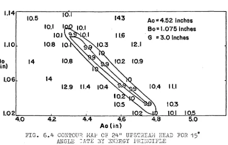
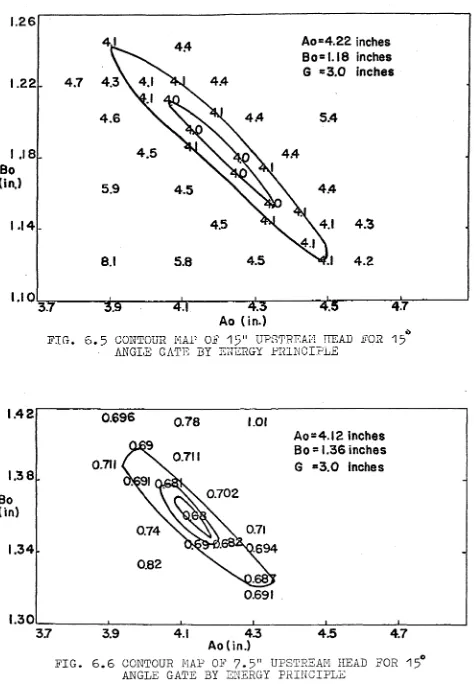
6,3 Contour Maps

The summation of squares of energy deviations along the

downstream surface elements for each pair-of (A0 » B0 ) was

plotted on a graph of A Q vs B and a contour map was drawn

for many pairs of. (A0f B0 ), From the closed contour map,

a pair of (A0 , B0 ) corresponding to the minimum summation of

squares of energy deviations was obtained.

The contour maps for the various types of gates and various

upstream heads are shown in Fig. 6.1 to Fig. 6.18.

6.4- Downstream Free Surface Profile

The calculation of donwstream free surface profile was

based on the pair of (Ao. Bo) which gave the minimum error in

the finite element method.

All the graphs of downstream free surface profiles are

shown in Fig. 6.10, Fig. 6.11 and Fig. 6.12.

(60)

T A B L E 6 . 2

4 1

COMPUTED C c AND C D BY ENERGY METHOD

No.

of

run 0

Total

No.of

ele

ments

Total

No. of

unk

nown

nodes U/S

head

(IN)

u>

No. of

iter

ation

No. of

D/S

sur

face

ele

ments

6 *

A o B o C c C D

1 0° 61 18 24.0 1.2 ₁₃ 6 _{6.4oo 3 . H 7} 1 . 1 7 0 _{0.610 0.5‘}

2 0° 61 18 15.0 1.2 ₁₃ 6 3 . 1 0 0 3.130 1.200 0 . 6 0 0 _o.5<

3 0° 61 18 7.5 1.2 13 6 0 .I89 3.130 1.197 0 . 6 0 1 0.5:

4

i f

93 28 24.0 1.2 16 10 8 . 9 0 0 4.520 1.075 0.664 0 .6;

5

I f

93 28 15.0 1.2 15 10 4.000 4.220 1.180 0 . 6 3 6 o.5(

6

i f

91 28 7.5 1.2 15 10 0 . 6 8 0 4.120 1 . 3 6 0 0.58? 0.5:

7 30° 93 28 24.0 1.2 15 10 6 . 5 0 0 4.300 1.150 0 . 6 7 6 0.

6!

8 30° ₉₃ 28 15.0 1.2 14 10 3.200 4 . 4 9 6 1.136 0.679 0.6;

9 00° 93 28 7.5 1.2 16 10 0.530 4.570 1.210 0 . 6 5 8 0.5!

(61)

T A B L E 6 . 3

COMPUTED C c AND CD BY MOMENTUM METHOD

4 2 No. of run 9 Total No. of ele ments -Total No .of unk nown nodes u/s head (IN) U> No.of iter ation: No. of D/S sur face ele ments