Volume 2006, Article ID 90716, Pages1–9 DOI 10.1155/ASP/2006/90716
Eigenspace-Based Motion Compensation for
ISAR Target Imaging
D. Yau, P. E. Berry, and B. Haywood
Electronic Warfare and Radar Division, Department of Defence, Defence Science and Technology Organisation (DSTO), Australian Government, Edinburgh, South Australia 5111, Australia
Received 8 June 2005; Revised 17 October 2005; Accepted 24 November 2005
A novel motion compensation technique is presented for the purpose of forming focused ISAR images which exhibits the robust-ness of parametric methods but overcomes their convergence difficulties. Like the most commonly used parametric autofocus techniques in ISAR imaging (the image contrast maximization and entropy minimization methods) this is achieved by estimating a target’s radial motion in order to correct for target scatterer range cell migration and phase error. Parametric methods generally suffer a major drawback, namely that their optimization algorithms often fail to converge to the optimal solution. This difficulty is overcome in the proposed method by employing a sequential approach to the optimization, estimating the radial motion of the target by means of a range profile cross-correlation, followed by a subspace-based technique involving singular value decomposi-tion (SVD). This two-stage approach greatly simplifies the optimizadecomposi-tion process by allowing numerical searches to be implemented in solution spaces of reduced dimension.
Copyright © 2006 D. Yau et al. This is an open access article distributed under the Creative Commons Attribution License, which permits unrestricted use, distribution, and reproduction in any medium, provided the original work is properly cited.
1. INTRODUCTION
Imaging of targets using inverse synthetic aperture radar (ISAR) exploits the large effective aperture induced by the relative translational and rotational motion between radar and target and has the ability to create high-resolution im-ages of moving targets from a large distance. The technique is independent of range if rotational motion is significant, and it therefore has good potential to support automatic tar-get recognition. A tartar-get image is formed by estimating the locations of target scatterers in both range and cross-range but the scatterer motion needs to be compensated for in or-der to avoid image blurring which can occur due to scatterer migration between range cells and scatterer acceleration.
The common autofocusing methods can be categorized into parametric and nonparametric approaches. Computa-tionally, nonparametric methods are much more efficient and easy to implement. The compensation for translational motion normally comprises two separate steps: range cell realignment and phase-error correction. Range cell realign-ment is considered to be routine and is based upon, for in-stance, the correlation method (see Chen and Andrews [1]) or the minimum-entropy method (see Wang and Bao [2]). Phase autofocus is more stringent in its requirements and many nonparametric methods have been proposed, most of
which track the phase history of an isolated dominant scat-terer (prominent point processing (PPP), see Steinberg [3]) or the centroid of multiple well-isolated scatterers (multiple scatterer algorithm (MSA), see Carrara et al. [4], Haywood and Evans [5], Wu et al. [6], Attia [7]). The phase-gradient algorithm (PGA, see Wahl et al. [8]) is another popular non-parametric technique, which iteratively estimates the residual phase by integrating over range an estimate of its derivative (gradient). Because nonparametric methods are based on the assumption of well-isolated dominant scatterers, they do not perform satisfactorily in many practical situations. On the other hand, parametric methods (Berizzi and Corsini [9], Xi et al. [10], Wu et al. [11], and Wang et al. [12]) are much more robust but more numerically intensive.
Common parametric techniques that use a polynomial model to approximate the target’s translational motion and use an image focus criterion to estimate the model parame-ters are the image-contrast-based technique (ICBT, see [13]) and entropy-based technique (EBT, see [10,14]). The chal-lenge for autofocus is to devise algorithms which not only focus adequately for target recognition but are also both ro-bust and efficient. This generally involves a tradeoff, between efficiency and effectiveness.
image focus quality which is formulated as an objective func-tion. Depending on the order of the model, the search is nor-mally carried out over a two- or three-dimensional space. One major drawback of these methods is that the optimiza-tion algorithm (minimizaoptimiza-tion/maximizaoptimiza-tion routine or op-timizer) often converges to a suboptimal solution if the ob-jective function is highly multimodal or has a large number of local minima/maxima. Moreover, most deterministic op-timization methods, such as Newton, gradient, and so forth, are constrained by the fact that the objective function has to be continuously differentiable.
In summary, a successful convergence to the optimal so-lution and the numerical efficiency of the method very much depend on various factors in relation to the nature of the objective function, such as differentiability and continuity, number of local minima/maxima, as well as the robustness of the optimization algorithm, for example its sensitivity to the initial guessed value.
The motion compensation technique described in this paper is a parametric method that does not depend upon the assumption of prominent scatterers but estimates the target’s radial velocity based upon the composite of all of the target scatterers. It uses this to correct the data for the slant-range and cross-range phase errors due to the translational motion of the target, thereby significantly improving image quality.
In the proposed optimization procedure, the first-order and higher-order parameters of the target’s radial motion are estimated sequentially by means of a range profile cross-correlation and a subspace-based technique involving eigen-decomposition. By decoupling the first- and higher-order pa-rameter searches, the technique allows the optimizers (min-imization/maximization routines) to be implemented over spaces of lower dimension, and thus reduces the likelihood of converging to a suboptimal solution as encountered with other parametric methods. An overview of autofocus meth-ods is given by Xi et al. [10] and Li et al. [14], and a recent survey is presented by Berizzi et al. [15].
2. PROBLEM FORMULATION
Consider a target with complex reflectivity functionζ(r) in the imaging plane of the target’s frame of reference, that is, in slant-rangexand cross-rangey(seeFigure 1). The target motion with respect to the radar line of sight (RLOS) can be decomposed into radial motion of an arbitrary reference pointOon the target and rotational motion about the ref-erence point. LetR0(t) denote the radial distance ofOfrom the radar at timetthenOmay be chosen to be the origin of the target’s coordinate system (seeFigure 1).
If the radial motion of the target’s reference pointO(due to translational motion) is defined by the initial velocityv0r
and constant accelerationar, and if the target is rotating at
an angular velocity ofΩaboutO, then the distance from an arbitrary scatterer (xk,yk) on the target to the radar at timet
can be written as
Rk(t)=R0(t) +ΔRk(t), (1)
whereR0(t)=R0(0) +v0rt+art2/2 andΔRk(t)=xkcosΩt−
yksinΩt.
Scatterer on the target
Point of reference
Target RLOS
Radar
y
vt(t)
(x,y) x
r(t)
Ω
O
R0(t) R(t)
Figure1: System geometry.
Let us define the transmitted RF signal for a coherent processing interval (CPI) of periodTas the real part of
z(t)=u(t)e2π j f0t, (2)
where f0is the carrier frequency andu(t) is the complex en-velope of the waveform given byu(t)=A(t) exp{jφ(t)}, and with Fourier transformU(f), where A(t) andφ(t) are the amplitude and phase modulation of the signal, respectively. Then the received signal after demodulation and downcon-version to baseband can be written as
sR(t)= K
k=1 ζku
t−τk(t)
exp−j2π f0τk(t)
, (3)
whereK is the number of scatterers on the target,ζkis the
reflectivity of thekth scatterer which has local coordinates of (xk,yk) with respect toOand is of distanceRk(t) from the
radar,τk(t) is the delay function given byτk(t)=2Rk(t)/c,
andcis the velocity of light.
IfΩis small in comparison toT and the target’s radial displacement is negligible for the duration of fast time sam-pling, then we can write the Fourier transform of the received signal as
S(f,t)=U(f)
K
k=1 ζkexp
−2π j f τk(t)
, (4)
wheretnow refers to slow time, that is, pulse-to-pulse. The Fourier transform of the range profile, following the devel-opment in [9,16], is therefore
SR(f,t)=S
(f,t) U(f) =
K
k=1 ζkexp
−2π j f τk(t)
Nowτk(t)=2Rk(t)/c=(2/c)[R0(t) +ΔRk(t)], hence
SR(f,t)
=exp
−4π j f R0(t) c
K
k=1 ζkexp
−4π j fΔRk(t)
c ,
(6)
whereΔRk(t) ≈ xk−ykΩt, from which we see that phase
changes occur in slow time for each scatterer but that the phase changes associated with radial target motion are sep-arate from those associated with target rotation. The phase changes associated with the radial motion of the reference scatterer may therefore be corrected for by making the phase adjustment 4π j f R0(t)/cto each pulse in the frequency do-main. SinceR0(t)=R0(0) +v0rt+art2/2, we need to estimate
v0randarfor the reference scatterer.
The corrected range profile Fourier transform is then
SR(f,t)=exp
4π j f R0(t)
c SR(f,t)
=
K
k=1 ζkexp
−4π j fΔRk(t)
c ,
(7)
from which the realigned and phase-compensated range pro-file may be recovered by means of an inverse FT. Frequency estimation may then be performed in each range cell for cross-range velocity estimation. In a radar system, f andt take the digitized forms of f = fm (m = 1,. . .,M) and
t=pT(p=1,. . .,N), where fmis themth sample in the
fre-quency domain andTis the pulse repetition interval (PRI); MandNare the number of frequency samples and Doppler pulses, respectively.
The radial motion of the target has the effect of causing scatterers to migrate between range cells, and hence smear-ing of the image in the range dimension; whereas the 1/2art2
term alone causes nonlinear phase variation in slow time, and hence smearing of the image in the cross-range dimen-sion. If the length of the burst is sufficiently small compared with the rotation rate of the target, then the ykΩt term is
approximately linear and provides the Doppler information necessary for cross-range imaging.
3. VELOCITY AND ACCELERATION CORRECTION TECHNIQUE
The purpose of the present paper is to estimate the ra-dial velocity and acceleration so as to determine the de-layτ and hence correct for the phase in the data. The op-timization procedure comprises maximizing the objective functionsFv(v0r) and Fa(ar) separately for the single
vari-ablev0randarspaces, respectively, whilst keeping the other
motion parameter fixed. The objective functions are formu-lated in a way such that Fv(v0r)/Fa(ar) is relatively
invari-ant to the changes of the fixed parameterar/v0r. This not
only allows the optimization to be implemented solely in one-dimensional space, but also guarantees a fast conver-gence rate. The two-stage estimation technique procedure is
Initialize v0r&ar
Compute z(m,p)
ComputeFv(v0r) to estimatev0r
Fv(v0r) maximized?
Compute z(m,p)
ComputeFa(ar) to estimatear
Fa(ar) maximized?
Recompute z(m,p)
Successive estimates within error
bound?
Completed Yes
Yes
Yes No
No
No
Figure2: Flowchart showing the procedure for estimating velocity and acceleration.
summarized inFigure 2and as follows: initial estimation of velocity using a cross-correlation technique followed by es-timation of acceleration using a subspace-based approach. Further refinement is achieved as required by repeating the previous steps although in practice, at most only three itera-tions are required.
Denote the matrix of complex radar signals organized ac-cording to range cell and pulse, respectively, byz(m,p). For assumed values ofv0randar, the previously described
pro-cedure for range realignment and phase compensation is ap-plied to the recorded data of (6) . The range profilez(m,p) produced for range cellsm = 1,. . .,M and Doppler pulses p =1,. . .,Nis written as the inverse discrete Fourier trans-form of (6) after being adjusted for phase errors as follows:
z(m,p)=IDFTξv0r,a0r,pT
SR
fm,pT
, (8)
where ξ(v0r,a0r,p) = exp{−j4π f R0(v0r,a0r,pT)/c} is the
data, andR0is the corresponding radial range displacement of the target at timet=pTgiven some estimates of velocity and acceleration (v0r,a0r). In the following, it is shown how
the objective functions are formulated separately in terms of the parametersv0randa0rfor optimization.
The measure of how well the range realignment and phase compensation have been achieved is to compute the cross-correlation function r1,p(0) between the first range
profile (i.e., for the first pulse) and each of the remaining range profiles, and summing their moduli, thus
Fv
v0r
=
N
p=2
r1,p(0), (9)
wherer1,p(0)= M
m=1z∗(m, 1)z(m,p). The velocity estimate is that value ofv0r (given the correcta0r) which maximizes
the objective functionFv(v0r), either by a blind search
proce-dure or by formal optimization.
Following the improvement in the estimate of v0r, the
range realignment and phase compensation procedure are repeated. The accelerationaris estimated as follows. The
ac-celeration estimation technique exploits the fact that there will be many scatterers within the range cells occupied by the target to be imaged, which have a very similar radial ve-locity, although there will be a relatively small spread due to the superimposed varying cross-range rotational veloci-ties. Because we are concerned with estimating a radial ve-locity which changes within the duration of a burst, we take a fixed window within which it is assumed that the radial ve-locity is approximately constant and fit a linear model to all of the range cells. This produces a covariance matrix which is averaged over range cells. This has the advantage of incor-porating all of the energy from the target’s scatterers rather than having to find and depend upon one of a small number of prominent scatterers. As a general criterion for spectral estimation techniques, the size of a fixed window of pulses should be chosen to be greater than or equal to the size of the signal subspace.
A data matrix is constructed from range profiles taken within a window superimposed on the pulses in slow time, thus
Zi= ⎡ ⎢ ⎢ ⎣
z1,ni
· · · z1,ni+Nd−1
..
. . .. ... zM,ni
· · · zM,ni+Nd−1
⎤ ⎥ ⎥
⎦, (10)
where the window begins with thenith pulse and containsNd
pulses. Then the covariance matrixRi =(1/M)ZHi Zifor the
ith window is formed by averaging over the range cells. Sub-space theory tells us that the principal eigenvectors span the same subspace as the signal vectors. In general, we will not know the dimensions of these subspaces (except that their sum isNd), but it is sufficient for our purposes to identify the
dominant signals associated with the signal subspace through eigendecomposition.
Therefore, the covariance matrix is subject to the eigen-decomposition
Ri=ViΛiVHi , (11)
where the Λi = diag(λ1,λ2,. . .,λNd) is the diagonal ma-trix of eigenvalues with λ1 ≥ λ2 ≥ · · · ≥ λNd and Vi = [vi,1 vi,2 · · · vi,Nd] is the matrix containing all the corre-sponding eigenvectors.
Computationally, singular value decomposition (SVD) is a more practical approach to computing the set of eigenvec-tors directly from the data matrixZi = UiΣiVHi , whereUi
is anM-by-Munitary matrix,Σiis a diagonal matrix of the
formΛi=diag(σ1,σ2,. . .,σNd), andσk(1,. . .,Nd) are the sin-gular values which are related to the eigenvalues byλk =σk2.
The diagonal matrixΣi(Λi) is always full rank because of
re-ceiver noise. The noise power is small in comparison to the signal power, and thus the signal subspace can be determined by examining the singular values.
The assumption behind the method is that the principal eigenvectors contain the Doppler information for the dom-inant scatterers on the target for theith window. All of the scatterers will be subject to phase changes between pulses: one component will be a linear phase shift due to the com-mon initial velocityv0r and the other nonlinear phase shift
due to acceleration ar. This may be seen from the range
response function ζ0e−4π j f0/c(R0+v0rt+1/2art2) for the reference scatterer. The Doppler information implicit in two data ma-trices taken from different time intervals, sayZiandZi+j, will
differ by an amount proportional to the change in the veloc-ity or accelerationar. In mathematical terms, this difference
corresponds to the “rotation” of the signal subspace with re-spect to the origin of the vector space. However, when the acceleration has been correctly adjusted, the signal subspace or the principal eigenvectors associated with the windows should coincide (within an arbitrary phase).
We suppose that only two windows are chosen. A mea-sure of how well the principal eigenvectors coincide between the first and second windows of the burst is the sum of the moduli of their respective inner products:
Fa
ar
=
Np
k=1
vH
1,kv2,k, (12)
whereNpis the number of principal eigenvectors chosen to
represent the signal subspace. This objective functionFa(ar)
is to be maximized over ar. For simplicity, we choose the
eigenvector which corresponds to the largest eigenvalue for each window so thatFa(ar)= |vH11v21|. In fact, the number of windows chosen is arbitrary and is always a compromise be-tween accuracy and efficiency. For example, if we chooseNw
windows and use the first window as the reference, then the objective function is reformulated asFa(ar)=
Nw
i=1|vH11vi1|. It can be easily shown that the number of computer op-erations required for calculatingFv(v0r) isM(N−1) and for
Fa(ar) is approximately 4MNp2−4N3p/3 (the number of
op-eration required for SVD).
4. RESULTS
Table1: Radar parameters.
Pulse compression Stepped frequency
Number of sweeps 64
Number of transmitted frequencies 64
Centre frequency 10 GHz
Frequency step 2.34 MHz
Bandwidth 150 MHz
PRF 74.46 kHz
x y
4
4
4
4 3 3
3 3 3
3 2
2
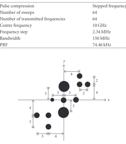
Figure3: Simulated target point reflector configuration.
the circles in the drawing. The relative sizes are 0.5, 1 and 2, respectively. The target is travelling towards the radar with an initial velocity of 5 m/s and with constant acceleration of 2 m/s2, with self-induced rotation of 0.16πrad/s.
Our technique is compared to Haywood-Evans MSA [5] and PGA [8] motion compensation techniques with a signal-to-noise ratio (SNR) of 20 dB. The results are shown in
Figure 4and it can be seen that the present technique gen-erates a better focused image than the other techniques. Us-ing our technique, v0r andar are estimated to be 5.15 m/s
and 2 m/s2, respectively. For a detailed examination of the behavior of the objective functions, Fv andFa are plotted
against v0r and ar in Figures 5(a) and5(b). The objective
functions are also plotted with respect to fixed parameters in Figures6(a)and6(b). It can be seen that their variation is rel-atively insignificant as compared to the previous figures. An-other similar set of data but with lower signal-to-noise ratio (SNR=10 dB) was tested and used for comparison between the different techniques. The resulting images are shown in
Figure 7. Again our technique outperforms MSA and PGA. In computing these plots, the subspace technique was implemented using two windows of size 8. Only the eigen-vector which corresponds to the largest eigenvalue was used to maximize Fa(ar). The computation time taken was less
than 1 second on a Pentium IV 2.5 GHz computer and took roughly 10 times longer than the PGA method. This is com-parable to the ICBT and EBT methods as stated in [15]. The algorithm was run on Matlab and the maximization was implemented by a toolbox function calledfminbnd(used to minimize the negative of the objective functions). It took
only two iterations for the optimization algorithm (Figure 2) to converge to the desired results. On average, it required about 10 iterations forfminbndto maximize each objective function.
Next, we show an experimental example of a Boeing 737 (Figure 8) ISAR image reconstructed using MSA and the proposed subspace algorithm in Figure 9. The radar is at ground level and the parameters are lowest frequency = 9.26 GHz, frequency step = 1.5 MHz, range resolution =0.78 m, PRF/sweep rate=20 kHz/156.25 Hz; and the size of the data matrix is 64 by 64. Again it is seen that the pro-posed technique produces a much better image.
5. CONCLUSIONS
This paper has proposed a new parametric autofocus method for simultaneously realigning range and compensating for phase by estimating radial velocity and acceleration using a combination of range profile correlation for velocity estima-tion and subspace eigenvector rotaestima-tion for acceleraestima-tion esti-mation. The method does not suffer from the limitation of assuming the existence of prominent scatterers as in other nonparametric methods.
45 40 35 30 25 20
Range (m) −15
−10 −5 0 5 10 15
Do
p
p
le
r
fr
eq
u
en
cy
(Hz)
−15 −12 −9 −6 −3 0 dB
(a)
60 50 40 30 20 10 0
Range (m) −30
−20 −10 0 10 20 30
Do
p
p
le
r
fr
eq
u
en
cy
(Hz)
−24 −19.2 −14.4 −9.6 −4.8 0 dB
(b)
45 40 35 30 25 20
Range (m) −15
−10 −5 0 5 10 15
Do
p
p
le
r
fr
eq
u
en
cy
(Hz)
−15 −12 −9 −6 −3 0 dB
(c)
Figure4: Range-Doppler image of simulated target (SNR=20) using (a) MSA technique [5]; (b) PGA technique [8]; (c) proposed subspace technique.
10 9 8 7 6 5 4 3 2 1 0
v0r 30
35 40 45 50 55 60
Fv
(a)
4 3.5 3 2.5 2 1.5 1 0.5 0
ar 0.1
0.2 0.3 0.4 0.5 0.6 0.7 0.8 0.9 1
Fa
(b)
4 3.5 3 2.5 2 1.5 1 0.5 0
ar 30
35 40 45 50 55 60
Fv
(a)
10 9 8 7 6 5 4 3 2 1 0
v0r 0.1
0.2 0.3 0.4 0.5 0.6 0.7 0.8 0.9 1
Fa
(b)
Figure6: Plots of objective functions against the fixed parameters (a)Fvversusar(v0r=5.15 m/s2) and (b)Faversusv0r(ar=2 m/s2).
45 40 35 30 25 20
Range (m) −15
−10 −5 0 5 10 15
Do
p
p
le
r
fr
eq
u
en
cy
(Hz)
−15 −12 −9 −6 −3 0 dB
(a)
60 50 40 30 20 10 0
Range (m) −30
−20 −10 0 10 20 30
Do
p
p
le
r
fr
eq
u
en
cy
(Hz)
−24 −19.2 −14.4 −9.6 −4.8 0 dB
(b)
45 40 35 30 25 20
Range (m) −15
−10 −5 0 5 10 15
Do
p
p
le
r
fr
eq
u
en
cy
(Hz)
−15 −12 −9 −6 −3 0 dB
(c)
Figure8: Schematic of a Boeing 737 (top view).
60 50 40 30 20 10 0
Range (m) −30
−20 −10 0 10 20 30
Do
p
p
le
r
fr
eq
u
en
cy
(Hz)
−24 −19.2 −14.4 −9.6 −4.8 0 dB
(a)
60 50 40 30 20 10 0
Range (m) −30
−20 −10 0 10 20 30
Do
p
p
le
r
fr
eq
u
en
cy
(Hz)
−24 −19.2 −14.4 −9.6 −4.8 0 dB
(b)
Figure9: ISAR image of a Boeing 737: (a) MSA technique [5] (3 reference cells used); (b) proposed subspace technique.
REFERENCES
[1] C.-C. Chen and H. C. Andrews, “Target-motion-induced radar imaging,”IEEE Transactions on Aerospace and Electronic Systems, vol. 16, no. 1, pp. 2–14, 1980.
[2] G. Wang and Z. Bao, “The minimum entropy criterion of range alignment in ISAR motion compensation,” in Proceed-ings of the IEEE International Radar Conference, pp. 236–239, Edinburgh, UK, October 1997.
[3] B. D. Steinberg, “Microwave imaging of aircraft,”Proceedings of the IEEE, vol. 76, no. 12, pp. 1578–1592, 1988.
[4] W. C. Carrara, R. S. Goodman, and R. M. Majewski,Spotlight Synthetic Aperture Radar: Signal Processing Algorithms, Artech House, Boston, Mass, USA, 1995.
[5] B. Haywood and R. J. Evans, “Motion compensation for ISAR imaging,” inProceedings of Australian Symposium on Signal Processing and Applications (ASSPA ’89), pp. 113–117, Ade-laide, Australia, April 1989.
[6] H. Wu, D. Grenier, G. Y. Delisle, and D.-G. Fang, “Transla-tional motion compensation in ISAR image processing,”IEEE Transactions on Image Processing, vol. 4, no. 11, pp. 1561–1571, 1995.
[7] E. Attia, “Self-cohering airborne distributed arrays on land clutter using the robust minimum variance algorithm,” in Pro-ceedings of IEEE Antennas and Propagation Society Interna-tional Symposium (APS ’86), vol. 24, pp. 603–606, June 1986. [8] D. E. Wahl, P. H. Eichel, D. C. Ghiglia, and C. V. Jakowatz
Jr., “Phase gradient autofocus—a robust tool for high reso-lution SAR phase correction,”IEEE Transactions on Aerospace and Electronic Systems, vol. 30, no. 3, pp. 827–835, 1994. [9] F. Berizzi and G. Corsini, “Autofocusing of inverse synthetic
aperture radar images using contrast optimization,” IEEE Transactions on Aerospace and Electronic Systems, vol. 32, no. 3, pp. 1185–1191, 1996.
[10] L. Xi, L. Guosui, and J. Ni, “Autofocusing of ISAR images based on entropy minimization,”IEEE Transactions on Aerospace and Electronic Systems, vol. 35, no. 4, pp. 1240–1252, 1999. [11] H. Wu, D. Grenier, G. Y. Delisle, and D.-G. Fang,
“Transla-tional motion compensation in ISAR image processing,”IEEE Transactions on Image Processing, vol. 4, no. 11, pp. 1561–1571, 1995.
[13] F. Berizzi, E. Dalle Mese, and M. Martorella, “Performance analysis of a contrast-based ISAR autofocusing algorithm,” in
Proceedings of the IEEE International Radar Conference, pp. 200–205, Long Beach, Calif, USA, April 2002.
[14] J. Li, R. Wu, and V. C. Chen, “Robust autofocus algorithm for ISAR imaging of moving targets,”IEEE Transactions on Aerospace and Electronic Systems, vol. 37, no. 3, pp. 1056–1069, 2001.
[15] F. Berizzi, M. Martorella, B. Haywood, E. Dalle Mese, and S. Bruscoli, “A survey on ISAR autofocusing techniques,” in Pro-ceedings of IEEE International Conference on Image Processing (ICIP ’04), vol. 1, pp. 9–12, Singapore, October 2004. [16] D. A. Ausherman, A. Kozmer, J. L. Walker, H. M. Jones, and
E. C. Poggio, “Developments in radar imaging,”IEEE Trans-actions on Aerospace and Electronic Systems, vol. 20, no. 4, pp. 363–400, 1984.
D. Yaureceived the B.E. degree in electrical engineering from The University of Sydney, Sydney, Australia, and the M.Eng.Sc. and Ph.D. degrees in electrical engineering from The University of Queensland, Queensland, Australia. He is currently working as a Re-search Scientist at DSTO, Australia. His re-search interests include radar imaging and signal processing.
P. E. Berry works in the Electronic War-fare and Radar Division of DSTO and has interests in estimation, optimization, and control applied to microwave radar engi-neering. He has previously worked in re-search laboratories in the UK’s electricity supply industry on problems of computa-tional physics and power system optimiza-tion and control.
B. Haywood received a Bachelor of Engi-neering (with honours) degree in 1984 and a Master of Engineering Science degree in 1988, both from the James Cook University, North Queensland Townsville. In 1988, he started studying for a Ph.D. degree at the University of Newcastle, NSW, which he was awarded in 1992. Since 1988, he has been with the Electronic Warfare and Radar Di-vision (and its predecessors) of the Defence