Isogeometric Analysis Method for Solving Parabolic PDEs by Using Bivariate Spline

(1)

2019 International Conference on Information Technology, Electrical and Electronic Engineering (ITEEE 2019) ISBN: 978-1-60595-606-0

Isogeometric Analysis Method for Solving Parabolic PDEs by Using

Bivariate Spline

Kai QU* and Jia-wei XUAN

College of Science, Dalian Maritime University, Dalian, China

*Corresponding author

Keywords: Bivariate spline, Finite element, Parabolic pdes, Isogeometric analysis.

Abstract. In this paper, we study isogeometric analysis method for solving parabolic Pdes by using bivariate spline finite elements on domains defined by NURBS. We constructed bivariate spline proper subspace of S42,3((mn2)) which satisfies homogeneous boundary conditions on type-2 triangulations and quadratic B-spline interpolating boundary functions. A numerical test is solved to assess the accuracy of this method.

Introduction

Solving the parabolic pdes is much important and has recently been studied by several schorlars. There are lots of literatures devoted to it. Researchers can referred to [1] for excellent surveys. We review some methods referred in this paper.

Recent works indicate that isogeometric analysis method have added yet another dimension to spline’s use, especially the simulation and numerical modelling [2-4].Because of a strategy that can increase the regularity of functions through the mesh’s interfaces, and also to reduce the number of degrees of freedom, the isogeometric analysis method is undoubtedly the emergence [5]. More attempt show that the isogeometric analysis method which use geometric transformations and non uniform splines is much simpler for the other approaches [6]. Modern finite element techniques for parabolic pdes rely on ideas from differential geometry and more precisely on the existence of discrete spaces [7].Adaptive mesh refinement with spline method is not as straightforward which ideas have been proposed in [8]. This problem arises in more and more branches of science. In particular, plasma physics, heat conduction process, electrochemistry, semi-conductor modeling, control theory, inverse problems and biotechnology [9]. The analysis, development and implementation of numerical methods for the solution of suchparabolic pdes has received wide attention in the literature [10].

The organization of this paper is as follows. In Section 2, we construct the bivariate spline space. We write an solution to the general parabolic peds in a weak form in Section 3. Also in Section 3, we propose isogeometric analysis method for solving the weak solution. In Section 4, a numerical examples are given, also included in Section 4 is the comparison of the Isogeometric analysis method and other methods. A conclusion is drawn in Section 5.

Bivariate Spline Space

Splines are polynomials which are piecewise and have certain smoothness. The space of bivariate splines with degree kand smoothnessover is defined by

 :



 | | , 1, ,



i

k k

S   s C  sP i M

Here, the partition  of the domain is carried out by using a finite number of irreducible algebraic, and1,…, M , indicate cells of . We call type-2 triangulations are uniform type-2

(2)

[image:2.595.218.339.72.166.2]

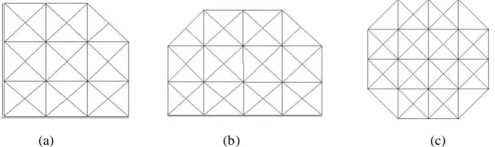
Figure 1. Uniform type-2 triangulation, m=4, n=4.

Now, we would like construct the locally supported splines in 2 (2)

4( mn)

S  which are consist of three

classes of _C2_{quartic B-spline bases. Also,}

) ( (2)

3 , 2 4 mn

S  can be costructed by adding the following two

continuous conditions: (i) s is _C2_{continuous on the rectangle grid segments; (ii)}_s_is_C3_continuous

on the diagonal grid segments. Next, we discuss locally supported splines in proper subspace of

) ( (2) 3 , 2 4 mn

S  with homogenous boundary conditions on type-2 triangulations. The basic idea is to use the

linear combination of B(x, y) in 2,3( (2))

4 mn

S  and their translations.

Let

, ( , ) ( , )

i j

B x y B mx i ny j .

Define the basis functions Bi y, ( , y)x as follows:

1,1 1,1 1,1 1, 1 1, 1 1,1 1,1 1,1 1, 1 1, 1 1, 1 1, 1 1, 1 1, 1 1, 1

1, 1 1,

( , ) ( , ) ( , ) ( , ) ( , )

( , ) ( , ) ( , ) ( , ) ( , y)

( , )

m m m m m

n n n n n

m n m n

B x y B x y B x y B x y B x y B x y B x y B x y B x y B x y B x y B x y B x y B x y B x B x y B

                                 

 1( , )x y Bm1,n1( , )x y Bm1,n1( , )x y Bm1,n1( , )x y       _ _ _  (1)

,1 ,1 , 1

, 1 , 1 , 1

1, 1, 1,

( , ) ( , ) ( , ), 2, 3, , 2

i i i

i m i m i m

j j j

n j n j n j

B x y B x y B x y i m

B x y B x y B x y j n

                          _ _ _ _  (2)

, ( , ) , ( , ), 2,3, , 2, 2,3, , 2

i j i j

B x y B x y i m j n (3)

B-spline functions in Equation.(1)-(3) are called corner, side and interior B-spline bases,

respectively. Their supports are shown in Figure 2. The B-spline functions are 1

C across the single

marked mesh lines and 0

C across the double marked mesh segments.

(a) (b) (c)

Figure 2. (a) Corner B-spline Basis (b) Side B-spline Basis (c) Interior B-spline Basis

It can be proved that B_{i j}_, ( , y)x : 1  i m 1,1  j n 1can only span the proper subspace of S₄2,3((2)_mn) with

homogenous boundary conditions on type-2 triangulations ( 2,3;0 (2)

4 ( mn)

S  for short).

Isogeometric Analysis Method for Solving Parabolic PDEs

[image:2.595.126.479.558.663.2]

(3)

y xx

u u  f , in, t0 (4)

0

u , on,t0 (5)

0 ( , 0)

u  u , in (6)

Eq.(4)-Eq.(6) can be given the following equivalent weak formulation: Find u:R_ H₀1( ) such that

( , ) (u v_t    u, v) ( , )f v , v H₀1( ) ,t0

0 ( , 0)

u  u

The Isogeometric Analysis Method is defined as follows: Let 0  t₀ t₁  t_l be a (not necessarily) partition of the positive t-axis R_into subintervals I_l (t_l_₁, ]t_l , and define with q a

nonnegative integer the corresponding set of piecewise polynomials of degree at most q in t with

values in H₀1

 

 by

1

. , 0

0

{ : | , ( ), 0,1, , , 1, 2, }

l

q i I i l i l

i

W v v a t a H i q l



 



    .

In this note we shall consider only the case q0, it means that the solution of problem Eq.(4)-Eq.(6) in each subintervals I_l (for some suitable) is not changed.

1

( , ) ( , ) ( , )

l

l l l l

I

U U _ v k U  v



f v dt,  v H₀1( ) ,l 1, 2, ,

0 0

U u ,

where k_l  t_l t_l_₁ is the length of the subinterval I_l. U_l is the numerical solution of Eq.(4)-Eq.(6) when tI_l.

Since 2,3;0

 

(2) 4 mn

S  can be embedded into H₀1

 

 , we can select it as the testing function space.

To find a solution 2,3;0

 

(2)

4

l mn

U S  such that

1

( , ) ( , ) ( , )

l

l l l l _I

U U_ v k U  v



f v dt,  v S₄2,3;0

 

(2)_mn .

It is equivalent to the following formula:

~ ~ ~

, , ,

1

( , ) ( , ) ( , )

l

s t s t s t l l l l _I

U U_ B k U B 



f B dt,

 

~

2,3;0 (2) , ₄

s t _mn

B S

   . (7)

By using the B-spline bases on S₄2,3;0

 

(2)_mn , we can write

 

1 1 ~

, , , 1 1 , m n i j l i j l

i j

U  B x y

 

 





,

and insert to Eq.(7), we have the following linear system

1 1 ~ ~ 1 1 ~ ~

, , ,

, , , , ,

1 1 1 1

~ ~

, ₁ ,

( , ) ( , )

( , ) ( , ), 1 1,1 1

l

m n m n

s t i j s t i j l i j l i j n

i j i j

s t _l s t I

B B k B B

f B dt U B s m t n

                      





(8)

Therefore, the coefficients _{i j l}_{, ,} can be determined by the system of linear equations Eq.(8).

Numerical Test

(4)

Let =（0, 1）（0, 1 ）, consider the linear parabolic equation 0,

y xx

u u  0 x 1, y0, with the following initial and boundary conditions:

( , 0) 1,

u x  0 x 1,

(0, ) (1, )

u y u y , y0,

Here, we choosem and n are 32 in spline space 2,3;0 (2)

4 ( mn)

S  . The exact solution ( , )u x y , the

approximate solution u x yˆ( , ) by using the isogeometric analysis method, the approximate solution ( , )

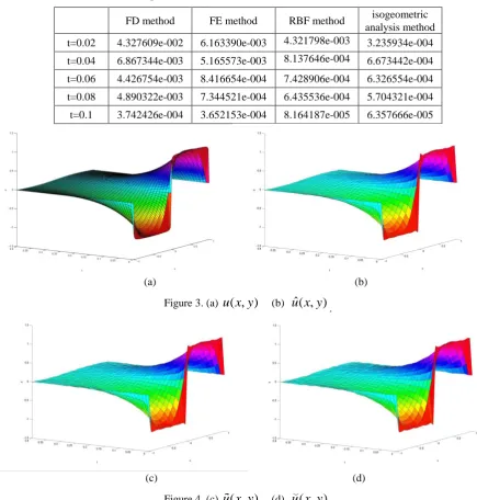
u x y by the finite difference method and the approximate solution ( , )u x y by using RBF method proposed are shown in Figure 3 and Figure 4.

[image:4.595.71.507.335.792.2]

The comparison of the numerical solutions by using the isogeometric analysis method, the RBF method, the finite difference method (FD method) and the finite element method (FE method) with its exact solutions at t=0.02, 0.04, 0.06, 0.08, 0.1 are displayed in Table 1, where x(0,1). Here, we enumerate the 2-norm errors between the exact solutions and the numerical solutions obtained from some methods. From Table 1, we can see that the GBC method and RBF method have fine accuracy. However, we have to choose 33 points to calculate the numerical solutions if we use the RBF method, it says, we should solve a system with the size of 33 33 .

Table 1. Comparison of numerical and exact solutions of numerical test.

FD method FE method RBF method isogeometric

analysis method

t=0.02 4.327609e-002 6.163390e-003 4.321798e-003 3.235934e-004

t=0.04 6.867344e-003 5.165573e-003 8.137646e-004 6.673442e-004

t=0.06 4.426754e-003 8.416654e-004 7.428906e-004 6.326554e-004

t=0.08 4.890322e-003 7.344521e-004 6.435536e-004 5.704321e-004

t=0.1 3.742426e-004 3.652153e-004 8.164187e-005 6.357666e-005

(a) (b)

Figure 3. (a) u x y( , ) (b) u x yˆ( , )_.

(c) (d)

(5)

Summary

In this paper, an isogeometric analysis method based on bivariate spline has been proposed to solve the general parabolic pdes. Here, bivariate spline proper subspace of 2,3

 

 2

4 m,n

S  satisfying

homogeneous boundary conditions on type-2 triangulations and quadratic B-spline interpolating boundary functions are primarily constructed. We could get the numerical solutions of parabolic pdes by using the spline in 2,3

 

 2

4 m,n

S  . The feasibility of the method is shown by a numerical test and the

approximated solutions are found to be in good agreement with the known exact solutions.

Acknowledgement

The authors acknowledge the National Natural Science Foundation of China (Grant: 11601056), the Science and Technology Foundation of Liaoning Province (201602076), the Fundamental Research Funds for the Central Universities (3132018229).

References

[1] M. Tatara, M. Dehghan, A method for solving partial differential equations via radial basis functions: Application to the heat equation. Engineering Analysis with Boundary Elements, 2010 34(3) 206-212.

[2] Buffa Annalisa, Giannelli Carlotta. Adaptive isogeometric methods with hierarchical splines: error estimator and convergence. Math. Models Methods Appl. Sci., 2016 26(1) 1–25.

[3] Buffa Annalisa, Garau Eduardo M.. Refinable spaces and local approximation estimates for hierarchical splines. IMA J. Numer. Anal. 2017 37(3) 1125–1149.

[4] Buffa Annalisa, Giannelli Carlotta. Adaptive isogeometric methods with hierarchical splines: Optimality and convergence rates. Math. Models Methods Appl. Sci., 2017 27(14) 2781–2802.

[5] Buffa Annalisa, Hernandez Vázquez Rafael, Sangalli Giancarlo, Beirão da Veiga Lourenço.

Approximation estimates for isogeometric spaces in multipatch geometries. Numer. Methods Partial Differential Equations, 2015 31(2) 422–438.

[6] Bressan Andrea, Buffa Annalisa, Sangalli Giancarlo. Characterization of analysis-suitable

T-splines. Comput. Aided Geom. Design, 2015 39 17–49.

[7] Toshniwal Deepesh, Speleers Hendrik, Hiemstra René R., Hughes Thomas J. R.. Multi-degree

smooth polar splines: a framework for geometric modeling and isogeometric analysis. Comput. Methods Appl. Mech. Engrg., 2017 316 1005–1061.

[8] Toshniwal Deepesh, Speleers Hendrik, Hughes Thomas J. R. Smooth cubic spline spaces on unstructured quadrilateral meshes with particular emphasis on extraordinary points: Geometric design and isogeometric analysis considerations. Comput. Methods Appl. Mech. Engrg., 2017 327 411–458.

[9] Kamensky David, Hsu Ming-Chen, Yu Yue, Evans John A., Sacks Michael S., Hughes Thomas J.

R.. Immersogeometric cardiovascular fluid-structure interaction analysis with divergence-conforming B-splines. Comput. Methods Appl. Mech. Engrg., 2017 314 408-472.

[10]Kruse R., Nguyen-Thanh N., De Lorenzis L., Hughes T. J. R. Isogeometric collocation for large