Efficient Generation of Power In Medium Voltage Direct Current Systems: Variable Speed Operation and Rectifier Considerations

University of South Carolina

Scholar Commons

Theses and Dissertations

2013

Fault Location in Power Networks Using

Synchronized Phasor Measurements

Cuong Nguyen

University of South Carolina

Follow this and additional works at:https://scholarcommons.sc.edu/etd

Part of theElectrical and Computer Engineering Commons

This Open Access Thesis is brought to you by Scholar Commons. It has been accepted for inclusion in Theses and Dissertations by an authorized administrator of Scholar Commons. For more information, please [email protected].

Recommended Citation

Nguyen, C.(2013).Fault Location in Power Networks Using Synchronized Phasor Measurements.(Master's thesis). Retrieved from

F

L

P

N

S

P

M

by

Cuong Nguyen

Bachelor of Science

Hanoi University of Science and Technology, 2009

Submitted in Partial Fulfillment of the Requirements

For the Degree of Master of Science in

Electrical Engineering

College of Engineering and Computing

University of South Carolina

2013

Accepted by:

Charles Brice, Director of Thesis

Enrico Santi, Reader

ii

iii

A

I would like to express my deepest appreciation to my advisor, Dr. Charles Brice.

Without his guidance and support, my graduate studies at University of South Carolina

would not have been completed. I would like to thank Dr. Enrico Santi for serving as my

thesis committee member and for the knowledge he provided during his classes and

during my thesis preparation. I would also like to thank Dr. Yong-June Shin for his

support throughout the course of my studies.

I would like express my gratitude to my fellow graduate students and friends in Power

and Energy group. Much appreciation also goes go to faculty and staff members at

Department of Electrical Engineering, University of South Carolina.

Finally, I would like to thank my parents and my brother whose love, support and

iv

A

Faults in electric power systems can lead to cascading power outages which cause

tremendous loss to the economy and affect people’s lives. Technical reports of recent

blackout events in the United States pointed out the lack of situational awareness as one

of the main causes of widespread outages. Time synchronized phasor measurement is

recommended as a technology that can improve the monitoring of power system

condition. By knowing exactly where a fault occurs, necessary actions can be taken in a

timely manner and thus, damage caused by that fault can be limited. In this thesis, first, a

method for precise frequency and phasor measurement is proposed. This novel method

bases on the linear combination of selected Discrete Fourier Transform terms and is able

to eliminate estimation error at off-nominal frequency. Second, the thesis presents a

method to locate fault in power network using voltage and current phasor measurements.

This fault location method involves the calculation of impedance matrix when network

topology changes during fault and fault location is found by matching the calculated

values of voltage and current phasors with its real world measurements. The proposed

method is implemented in MATLAB and is demonstrated in three example networks

simulated in PSCAD.

v

T

C

ACKNOWLEDGEMENTS ... iii

ABSTRACT ... iv

LIST OF TABLES ... vii

LIST OF FIGURES ... viii

CHAPTER1:INTRODUCTION ... 1

CHAPTER2:TIME SYNCHRONIZED PHASOR MEASUREMENTS ... 4

2.1 PHASOR MEASUREMENT UNIT ... 4

2.2 PHASOR ESTIMATION USING DISCRETE FOURIER TRANSFORM ... 7

2.3 FREQUENCY ESTIMATION ... 11

CHAPTER3:NOVEL METHOD FOR PRECISE FREQUENCY MEASUREMENT ... 15

3.1 FOURIER SERIES OF A PERIODIC CONTINUOUS TIME SIGNAL AT OFF NOMINAL FREQUENCY ... 16

3.2 DISCRETE FOURIER TRANSFORM AT OFF NOMINAL FREQUENCY ... 18

3.3 LINEAR COMBINATION OF DISCRETE FOURIER TRANSFORM TERMS ... 19

3.4 SELECTION OF DISCRETE FOURIER TRANSFORM TERMS ... 22

vi

4.1 OVERVIEW OF FAULT LOCATION IN POWER SYSTEM ... 28

4.2 NETWORK IMPEDANCE MATRIX CALCULATION ... 33

4.3 FINDING FAULT AS A NON-LINEAR LEAST SQUARES PROBLEM ... 39

CHAPTER5:TEST CASES IN PSCAD AND RESULT ... 45

5.1 6BUS NETWORK CASE ... 45

5.2 SINGLE CIRCUIT LINE CASE ... 51

5.3 DOUBLE CIRCUIT LINES CASE... 60

CHAPTER6:CONCLUSION AND FUTURE WORK ... 66

6.1 CONCLUSION ... 66

6.2 FUTURE WORK ... 67

vii

L

T

Table 3.1 Selection of DFT terms ... 24

Table 5.1 Voltage sources in 6 bus system ... 46

Table 5.2 Load in 6 bus system ... 46

Table 5.3 Line parameters... 47

Table 5.4 Fault location and fault resistance... 51

Table 5.5 6 bus system fault location result ... 51

Table 5.6 Single circuit line case ... 53

Table 5.7 Single circuit line case model ... 59

Table 5.8 Single circuit line fault location result ... 60

Table 5.9 Double circuit lines case ... 61

Table 5.10 Equivalent model of the double circuit lines case ... 64

viii

L

F

Figure 2.1 Configuration of a Phasor Measurement Unit... 5

Figure 2.2 Phasor Measurement Units in North American Power Grid ... 6

Figure 2.3 Phasor diagram ... 7

Figure 3.1 Maximum error of different frequency estimation methods ... 25

Figure 3.2 Maximum error of different frequency estimation methods ... 26

Figure 3.3 Frequency estimations of transient signal ... 27

Figure 4.1 Circuit diagram of faulted line ... 29

Figure 4.2 Lattice diagram for fault on transmission line ... 31

Figure 4.3 Faulted line ... 35

Figure 4.4 Faulted system ... 38

Figure 4.5 Data fitting using linear least square ... 40

Figure 4.6 Solving non-linear equations ... 41

Figure 5.1 6 bus system ... 46

Figure 5.2 Instantaneous current in line 1 – 2 ... 48

Figure 5.3 Voltage and current phasors at bus 1 ... 49

ix

Figure 5.5 Single circuit case ... 52

Figure 5.6 Stages of a fault ... 54

Figure 5.7 Voltage and current phasors at bus A ... 58

Figure 5.8 Voltage and current phasors at bus B ... 58

Figure 5.9 Double circuit lines test case ... 61

1

CHAPTER

1

1.

I

Electric power systems have been changing to meet the growing need of electricity.

The growth of electric energy consumption in the United States is 2.1% per year from

1980 to 2000 [4].While the energy demand is increasing, the transmission systems is

stressed harder since adding new transmission lines is difficult. Legal issue, concern

about environmental impact, land availability and others make the expansion of

transmission network a complicated process. At the same time, the aging of grid

infrastructure increases the system’s vulnerability to failure. Strengthening the U.S. grid

is now an urgent need as its failure can cause tremendous loss to the economy and affect

people life. The Northeast blackout of 2003 affected approximately 50 million people,

caused disruption in power generation, water supply, transportation, communication and

other industries. The cascading outage was initiated in Ohio amid high electrical demand.

Investigation stated that a transmission line went out of service due to tree contact and

highlighted the inadequate situational awareness as one of the causes lead to the blackout

[1].

The spread of cascading outage in future can be limited by correcting its direct causes:

the lack of situational awareness. Technical analysis of the Northeast blackout of 2013 by

North American Electric Reliability Council recommended installing additional

2

monitoring of power system condition. As the number of phasor measurement units

deployed is increasing, numerous algorithms have been proposed to utilize the

information obtained. Synchrophasor measurements can be used in applications such as

state estimation, disturbance monitoring, post disturbance analysis, adaptive protection,

real time automated grid control, etc. [5].

Dealing with fault in transmission and distribution lines is always a part of power

system’s operation. Faults are caused by many reasons such as lightning, rain, short

circuit caused by insulation break down, tree touching, etc. When a fault occurs,

protection devices will response to the disturbance created by that fault and faulted line

may be taken out of service. Protection devices are coordinated in the way that provides

maximum sensitivity to fault and undesirable conditions but their operation on

permissible conditions have to be avoided, as mentioned by Blackburn in [6]. A fault

locator that provides the exact location of fault can enhance the operation of protection

system. Series circuit breaker trips that lead to blackout in large area can be prevented if

fault location is identified quickly. For long transmission lines, fault locator can reduce

the labor required for maintenance and restore the service quicker since patrol is not

needed. An effective fault locator can help minimize the damage caused by a fault and

improve the quality of service for the customer.

Performance of fault location devices currently used in power system can be enhanced

with the new data provided by phasor measurement units. In this thesis, chapter 2 and

chapter 3 will discuss synchrophasor measurements and chapter 4 and chapter 5 focus on

the using of synchrophasor measurements to find fault location. Chapter 2 of this thesis is

3

measurement unit and its phasor and frequency estimation algorithms is discussed. The

presented estimation algorithms are based on calculation of Discrete Fourier Transform

term at fundamental frequency. In chapter 3, limitation of the classical frequency

estimation method is analyzed. Mathematic derivation of Discrete Fourier Transform

explains the error of classical method for input signal at off-nominal frequency. Base on

the analysis, a novel frequency estimation method using linear combination of Discrete

Fourier Transform terms at selected frequencies is proposed. The idea of this method is to

calculate the coefficients of the linear combination in order to reduce the error caused

when input signal’s frequency is not nominal. Chapter 4 discusses the issue of fault

location in power systems. First, an overview of fundamental fault location techniques is

provided. Then, we present the method to locate fault at power network level using

voltage and current phasor measurements. The principle of this method is to match the

calculated values of voltage and currents at certain buses and lines with the real world

measurements of these voltages and currents. This fault location method involves the

calculation of impedance matrix when network topology changes and matching problem

is solved by non-linear least squares. This method is applied to three example cases in

chapter 5. The three example cases are 6 bus system, single circuit line and double circuit

lines. The proposed algorithms are tested using PSCAD simulations. This chapter also

presents the calculation of equivalent model for the case of single circuit line and double

4

CHAPTER

2

2.

T

S

P

M

Voltage and current phasor information are important to power system monitoring and

control. A change in magnitude or phase angle can indicate a fault on transmission line,

generator loss, load change, etc. However, as measurements in power systems are

transmitted to operation centers from various locations across a large geographical area,

the report delay caused by communication decrease the accuracy of obtained information.

Using voltage and current phasors without knowing exactly the moment it is measured

can lead to the wrong interpretation of the data and it can diminish the ability to take

control action when an event happens. Fortunately, with the development of Global

Positioning System (GPS), high performance micro-processor and high bandwidth

communication, the phasor and other information can be synchronized with the accurate

time frame and transmitted to across the long distance. Phasor measurement unit (PMU)

was invented in 1988 by A.G. Phadke and J.S. Thorp at Virginia Tech. The device

measures real-time phasors of electrical waveforms in power systems using a common

time source (GPS) for synchronization [15]. In this chapter, PMU and its applications

will be briefly discussed. Following it is the basic algorithms for phasor and frequency

estimation used in PMU.

P

M

U

2.1.

5

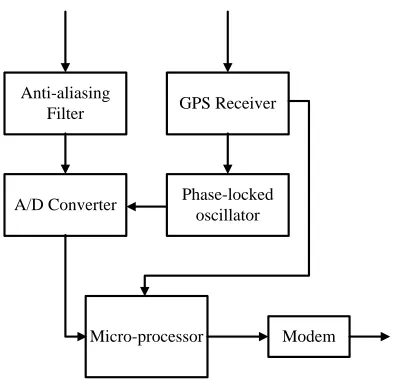
instrument transformers which convert the magnitude of signals to the working range of

the PMU. Before the analog signal is converted to digital form, it is pre-processed by the

anti-aliasing filter. The anti-aliasing filter ensures that input of A/D converter has

maximum frequency smaller than haft the sampling rate, which is the Nyquist frequency.

Using the anti-alias filter will minimize the effect of high frequency noise in the digital

signal.

Anti-aliasing Filter

A/D Converter

Micro-processor

Phase-locked oscillator GPS Receiver

Modem

Figure 2.1: Configuration of a Phasor Measurement Unit

The sampling clock is synchronized with GPS clock pulse. GPS stands for Global

Positioning System which is the system of satellites that provides precise location and

time information. GPS information has been used widely in both military and civilian

applications. Application utilizes location information provided by GPS can be seen daily

like cell phones and cars. For the PMU, the GPS satellites provide the one pulse per

second. Signal from the satellites is received by the GPS Receiver and it will convert the

6

numbers represent the input waveforms are stamped with the time frame synchronized

with GPS clock pulses. The phasors of input signals are then computed by the

micro-processor. The classical method for phasor estimation is described in the next section.

The estimates are time stamped and are transmitted to higher level of monitoring system

through the modem. Frequency, rate of change of frequency, flag (to indicate bad data)

can also be included.

Figure 2.2: Phasor Measurement Units in North American Power Grid

The number of PMUs installed in North American power grid has been increasing. The

deployment of PMUs across the network enables a better way to monitor modern power

systems, called Wide Area Monitoring (WAMS). In supervisory control and data

acquisition system (SCADA) which monitors traditional power system, measurements

7

and other important information are updated to the center once every two to four seconds

[16]. In Wide Area Monitoring system, measurements from PMUs can be updated at a

rate of once every one or two cycles, which is equal to 30 or 60 updates a second. This

higher rate of report enables the monitoring system to record faster dynamic behavior in

power systems.

P

E

D

F

T

2.2.

𝐴 2

𝜔0𝑡 + 𝜑0 Imaginary

axis

Real axis

𝐴

2𝑐𝑜𝑠 𝜔0𝑡 + 𝜑0

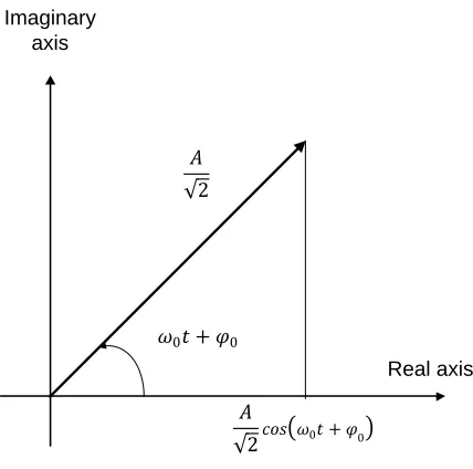
Figure 2.3: Phasor diagram

The term phasor was first introduced by C. P. Steinmetz in 1893. Phasor is the vector

representing a sinusoidal function whose frequency and amplitude are time invariant.

Phasors are used to represent current and voltage signals in power systems. Signal

𝑡 𝐴𝑐𝑜𝑠 𝜔 𝑡 𝜑 can be represented by a vector in complex coordination with

amplitude

and phase angle 𝜔 𝑡 𝜑 (Figure 2.3). Phasor can be expressed in polar

form

𝜔 𝑡 𝜑 or exponential form

8 form

𝑐𝑜𝑠 𝜔 𝑡 𝜑 𝑠 𝜔 𝑡 𝜑 . When the phasor is referred to not in a

specific time, the time dependent part of the phase angle can be neglected. It can be

simply written as

𝜑 in polar form. Now the phasor becomes a time invariant vector,

assuming the system is in steady state. This makes the calculation much easier compared

to the using of instantaneous voltage and current signals. In this thesis, however, the

phasor is referred to as a time varying quantity because it is intended to be used in power

system monitoring.

2.2.1. PHASOR ESTIMATION OF NOMINAL FREQUENCY SIGNAL

Consider the input of the estimator is an ideal sinusoidal signal at nominal

frequency . Angular frequency is 𝜔 .

𝑡 𝐴𝑐𝑜𝑠 𝜔 𝑡 𝜑 (2.1)

The signal is sampled at a sampling frequency which is a multiple of nominal

frequency . For current and voltage waveforms of electric grid, the nominal

frequency is 50Hz in most part of the world and is 60 Hz in the United States. This

allows PMU designers to select sampling frequency for each system. The sampled data of

input signal is:

𝐴𝑐𝑜𝑠 𝜔 𝜑

𝐴𝑐𝑜𝑠 ( 𝜑 ) (2.2)

Consider the first cycle of input signal, which is the first N samples from

to . The fundamental component of this data window is computed using

9

∑

𝐴

∑ (𝑐𝑜𝑠 ( 𝜑 ) 𝑐𝑜𝑠 ( ) 𝑐𝑜𝑠 ( 𝜑 ) 𝑠 ( ))

𝐴

∑ (𝑐𝑜𝑠 (

𝜑 ) 𝑐𝑜𝑠 𝜑 𝑠 ( 𝜑 ) 𝑠 𝜑 )

(2.3)

Because the summation ∑ 𝑐𝑜𝑠 ( 𝜑 ) and ∑ 𝑠 ( 𝜑 ) are equal to

zero, (2.3) becomes:

𝐴 (2.4)

As the phasor representation is defined in 2.1, we need to adjust equation (2.3) to

calculate the phasor representation of data window or 𝑡 [ ].

∑

(2.5)

The phasor representation of the sampled signal can be calculated using the above

formula simply by moving the data window on time domain. This is called non-recursive

update method. For this method, phasor representation of each data window is calculated

independently. As a result, error of estimation does not accumulate.

∑

(2.6)

Another method is recursive updates. For this method, phasor representation of a data

10 formula can be derived from (2.6):

∑

( ∑

)

( )

(2.7)

Using recursive update method can reduce the computation burden as there is no need

to calculate the loop . However, because the error is

added in each update, the phasor estimation obtained by this method is not reliable. This

accumulated error can be reduced by calculating a new phasor representation using

non-recursive method after repeat the non-recursive updates a certain times.

2.2.2. PHASOR ESTIMATION OF OFF-NOMINAL FREQUENCY SIGNAL

Now, consider the input of the phasor estimator is an ideal sinusoidal signal with

frequency . Angular frequency is 𝜔 .

𝑡 𝐴𝑐𝑜𝑠 𝜔 𝑡 𝜑 (2.8)

The signal 𝑡 is sampled with frequency . This means

𝐴𝑐𝑜𝑠 𝜔 𝜑 (2.9)

Using non-recursive method described in 2.2.1, the estimated phasor representation of

11 𝐴 ∑ 𝐴 _∑ ( ₎ 𝐴 _∑ ( ₎ (2.10) with ∑ ( ) ∑ ∑ ( ) ∑

Assuming the frequency 𝜔 is estimated accurately, and can be computed. In

(2.10), is known ( is calculated using non-recursive update method (2.5)). What we

need to do is to find phasor . (2.10) is re-written as:

{ _(2.11)

From (2.11), phasor is obtained as:

(2.12)

F

E

2.3.

12

governor at each generator will response to changes in the network to balance the input

mechanical power and the generated power. As a result, events like fault on transmission

lines, load changes, generator loss, etc. can be characterized by looking at the frequency

waveforms.

Historically, frequency in power systems is measured using mechanical speed sensor.

Devices are installed at power plants to measure speed of rotation of generators. This

limits the frequency measurement at the generator site. In modern power systems,

frequency can be measured at any point throughout the network. Instantaneous voltage

waveforms are recorded at high sampling rate and there are many different methods to

estimate the frequency digitally. Frequency estimation method using phasor angle is

described in this section.

Using non-recursive update method, the phasor is estimated from a data window which

has length equal to one cycle of nominal frequency using (2.6). The estimated phasor

obtained from (2.6) depends on the input signal’s frequency 𝜔 and the sampling

rate , which is related to the nominal frequency

𝐴

𝐴

(2.13)

is summation of two addends, one is proportional to and the other is

13

(2.14)

(2.15)

(3.1) and (3.2) shows that when the frequency of input signal approaches nominal

frequency, approaches the accurate value of phasor representation

_.

Define is the angle of complex number , we have the approximation:

𝜔 𝜑 _(2.16)

For the set of samples with , the angle of is:

𝜔 𝜑 (2.17)

From (2.16) and (2.17), the system frequency can be computed with 𝜔 , or:

𝑡 (2.18)

In commercial phasor measurement units (e.g. from ABB, SEL), rate of change of

frequency is estimated also:

𝑡 𝑡 (2.19)

One issue with this method is the existing of ripple caused by the component

proportional to in . To reduce the error, a digital filter may need to be

applied. The simplest filter can be used is an average filter. In [9], IEEE standard

C37.118.1-2011 defines two performance classes: P class and M class. Phasor

14

minimal report delay. P class on the other hand required fast response therefore mandates

no explicit filter. Comparison of maximum error of frequency estimated by different

15

CHAPTER

3

3.

N

M

P

F

M

As discussed in 2.2.2, the estimated phasor can be compensated assuming frequency is

known or is estimated accurately. Now, the accuracy of phasor measurement units

depends on how precise the frequency estimation is. In this section, the classical method,

using phase angle analysis, has been presented. Beside this method, many other

algorithms have been proposed to measure frequency in power system, includes least

square estimation, leakage coefficient measurement [10], Kalman filtering [13], Neural

Network [12] , Wavelet analysis [14], etc.

Most of the frequency measurement techniques use Discrete Fourier Transform at

fundamental frequency (nominal frequency of power system) and then using different

method to remove error caused by off nominal frequency and noise. Because the first step

is to calculate DFT component at nominal frequency, the accuracy of the above methods

decreases significantly when signal is highly off-nominal and especially under transient

condition.

In [10], instead of using DFT term at fundamental frequency only, the authors used the

leakage coefficient to calculate the variation of signal from nominal frequency:

∑ | | | |

| |

16

(3.2)

Since the relation in (3.2) is correct only if the signal is sinusoidal and the data window

starts from phase . As a result, a zero crossing detector must be applied. This makes the

method sensitive to noise.

In this chapter, the frequency components of an input signal at off nominal frequency

will be analyzed. Our analysis shows that by using several DFT terms in a linear

combination, the phase angle of input signal is estimated with smaller error. This also

means frequency estimate is more accurate.

F

S

P

C

T

S

O

3.1.

N

F

To measure the frequency which may be time variant, we will truncate the signal by a

rectangular window with length equal to nominal period and then, slide the window over

time. Without loss of generality, the signal was considered in one nominal period [ ].

Assume that in this time interval, the signal is an ideal sinusoidal function.

(3.3)

The rectangular window:

_{[ ]} { [ ] [ ]

(3.4)

Fourier transform of windowing function:

{ [ ] }

( ₎

17

According to modulation theorem, Fourier transform of truncated signal is:

{ 𝑡 𝑐𝑡[ ] 𝑡 }

𝐴 ( 𝜔 𝜔 )

𝜔 𝜔

𝐴

( 𝜔 𝜔 ₎

𝜔 𝜔 (3.6)

Consider ̃ 𝑡 is a periodic signal:

̃ 𝑡 𝑡 𝑐𝑡_{[ ]} 𝑡 𝑡 [ ] 𝑡 (3.7)

Fourier series of ̃ 𝑡 :

{ ̃ } { 𝑡 𝑐𝑡[ ] 𝑡 }_|

𝐴𝑠 ( 𝜔 𝜔 )

( )

( 𝜔_𝜔 )

𝐴

𝑠 ( 𝜔 𝜔 )

( )

( 𝜔_𝜔 ) _(3.8)

Note that the function ̃ 𝑡 is obtained by repeating the truncated part of 𝑡 in time

interval [ ]. Because the period of 𝑡 is , the function ̃ 𝑡 is not sinusoidal.

The Fourier series of a continuous signal cannot be computed in digital micro-processor.

However, as it will be shown in the following section, Fourier series expressed in (3.8) is

closely related to the discrete Fourier transform which can be computed from a set of

discrete samples.

18

𝑠 ( ) ( )

( ) has phase angle 𝜑

and the second term

𝑠 ( ) ( )

(

)

has phase angle (𝜑 ). When , the

magnitude of second term becomes 𝑠 ( )

(

)

which is nearly zero

since 𝑠 ( ) when is small. If the second term is equal to zero, the frequency

can be calculated simply from the phase angle of { ̃ }. However, depending on the

frequency of input signal, the second term still changes the phase angle of the summation

from 𝜑 . A method to eliminate the second term is discussed in the following

section.

D

F

T

O

N

F

3.2.

The signal 𝑡 in equation (3.3) is sampled with sampling frequency where

is nominal frequency.

𝐴𝑐𝑜𝑠 𝜔 𝜑 (3.9)

In discrete time domain, the periodic signal ̃ 𝑡 mentioned in (3.7) becomes

̃ [ ] (3.10)

Discrete Fourier Transform of ̃ :

̃ ∑

(3.11)

When (3.11) becomes the formula to calculate the phasor mentioned in previous

19 Substitute to (3.11):

̃ ∑ (𝐴 𝐴 ₎

(3.12)

Substitute 𝜔 and 𝜔 𝜔 𝜔 , after several steps of derivation we get:

̃ 𝐴

𝑠 ( 𝜔

𝜔 )

(

( ( ) )

𝑠 (( 𝜔_𝜔 ) ₎

( ( ) ₎

𝑠 (( 𝜔_𝜔 ) ))

(3.13)

(3.13) will become Fourier series of ̃ when the number of samples per cycle goes

to infinity . (3.13) is modified to obtained the form which is similar to the Fourier

series (3.8).

̃ ̃

𝐴

𝑠 ( 𝜔 𝜔 )

(

( ( ) )

𝑠 (( 𝜔_𝜔 ) ₎

( ( ) ₎

𝑠 (( 𝜔_𝜔 )

)) (3.14)

L

C

D

F

T

T

3.3.

From the equation (3.13) or (3.14), it can be seen that ̃ and ̃ are linear

combinations of two complex conjugates. This section will discuss how the combination

20

components; hence reduce the frequency estimation errors. The algorithm is basically

based on the following problem:

𝑐

𝑐

𝑐

𝑐 (3.15)

Find coefficient 𝑐 so that can be expressed as:

(3.16)

Generally, the numerator of S is a polynomial .

We need to find {𝑐 } so that and .

The solution for this problem is:

[ 𝑐 𝑐 𝑐 𝑐 ] [ ( ) ( ) ( ) ( ) ( ) ( ) ( ) ( ) ( ) ( ) ( ) ( ) ] [ ( ) ( ) ( ) ] (3.17)

Note that when is small, the value of is proportional to which is much very

small and can be considered zero. This characteristic will be used to eliminate the term

with phase angle (𝜑 ( ) ) in (3.14).

Suppose we select the set { }. Then we have the set of modified

discrete Fourier transform components { ̃ ̃ ̃ ̃ }. From the

definition of discrete Fourier transform, must be integer. A linear combination of

21

̃ ̃ ̃ with (3.18)

Substitute (3.14) to (3.18):

𝐴

𝑠 ( 𝜔

𝜔 )

(3.19)

with

𝜑 ( 𝜔 𝜔 )

(3.20)

𝑐

𝑠 (( 𝜔_𝜔 ) ₎

𝑐

𝑠 (( 𝜔_𝜔 ) ₎

𝑐

𝑠 (( 𝜔_𝜔 ) ₎ (3.21)

𝑐

𝑠 (( 𝜔_𝜔 ) ₎

𝑐

𝑠 (( 𝜔_𝜔 ) ₎

𝑐

𝑠 (( 𝜔_𝜔 ) ₎ (3.22)

To reduce the negative angle component in (3.20), should be minimized. Using the

result from (3.17) with 𝑠 (

22

Now, the frequency is calculated from phase angle of vector . Call is phase angle

of , the frequency estimate is:

𝑡 (3.24)

S

D

F

T

T

3.4.

This section will discuss the selection of discrete flourier transform terms (selection

[ 𝑐 𝑐 𝑐

𝑐 ] 𝑐𝑜𝑠 ( )

[

𝑐𝑜𝑠 ( )

𝑐𝑜𝑠 ( )

𝑐𝑜𝑠 ( )

𝑐𝑜𝑠 ( )_]

[

𝑐𝑜𝑡 ( ) 𝑐𝑜𝑡 ( ) 𝑐𝑜𝑡 ( )

𝑐𝑜𝑡 ( ) 𝑐𝑜𝑡 ( ) 𝑐𝑜𝑡 ( )

𝑐𝑜𝑡 ( ) 𝑐𝑜𝑡 ( ) 𝑐𝑜𝑡 ( )

𝑐𝑜𝑡 _{( ) 𝑐𝑜𝑡 ( ) 𝑐𝑜𝑡 (}

)_]

[

𝑐𝑜𝑡 ( )

𝑐𝑜𝑡 ( )

𝑐𝑜𝑡 ( )

𝑐𝑜𝑡 _{( )} ]

23

of { }) to archive accurate estimation. As described in section 3.3, with a set of DFT

terms selected, coefficient for each term can be found using (3.23) so that the

component in (3.19) is small and can be neglected. If is equal to zero then

there is no error caused by the off-nominal frequency. However, in reality, the accuracy

of frequency estimate depends on how small is in comparison with . Hence,

the selection of set { } has to consider the value of | |.

From practical point of view, the error of frequency estimate does not only come from

the off-nominal frequency of input signal but also from measurement noise or harmonic

components of voltage and current waveform. When there is noise, each DFT term

calculated by (3.14) will have an error added. Assuming the error added for each DFT

term is equal, the total error added to in (3.19) is proportional to sum of absolute value

of coefficients ∑ |𝑐|. Because we only need to calculate the phase angle of

component , the error of the estimation is proportional to ∑ | |.

The “normalized” values of | | and ∑ | | for some sets of { } is shown in Table 3.1.

“Normalized” here means values of | | and ∑ | | are divided to the corresponding value

when only the DFT term at fundamental frequency are used . Depending on each

particular application that the device is intended to be used, the designer may select the

appropriate set { }.Some applications may have better instrument transformer so the

noise is not a big problem. Other application may have higher noise level so the error

caused by noise in input signal is a concern. In addition, the burden of computation needs

to be considered as well. Including more DFT terms in the estimation also means higher

24

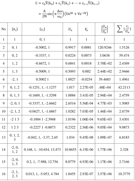
Table 3.1:Selection of DFT terms

̃ ̃ ̃

(

)

No { } {𝑐 } | | ∑ | 𝑐 |

1 1 0, 1 1 1 1 1

2 0, 1 -0.5002, 1 0.9917 0.0081 120.9246 1.5126

3 0, 2 -0.3337, 1 0.0224 0.0073 3.0638 59.474

4 1, 2 -0.6672, 1 0.6841 0.0018 3.70E+02 2.4369

5 1, 3 -0.5009, 1 0.5093 0.002 2.44E+02 2.9466

6 -2, 1 0.5002 1 1.0027 -0.0254 39.4683 1.4961

7 0, 1, 2 -0.1251, 1, -1.1237 1.017 2.27E-05 .48E+04 42.2113

8 0, 1, 3 -0.1669, 1, -1.3298 1.0084 3.41E-05 2.96E+04 2.4759

9 -2, 0, 1 -0.3337, 1, -2.6662 2.6516 5.56E-04 4.77E+03 1.5085

10 -2, 1, 2 -0.0627, 1, -1.6867 1.0282 7.03E-05 1.46E+04 2.6739

11 -2 1 3 -0.1004 1 -2.3968 1.0196 1.06E-04 9.65E+03 3.4301

12 1 2 3 -0.2227 1 -0.8873 0.2322 2.56E-06 9.05E+04 9.0873

13 0, 1, 2,

3 -0.042, 1, -3.37, 2.65 1.034 9.45E-08 1.09E+07 6.8183

14 -2, 0,

1, 2 0.168, 1, -10.654, 13.473 10.8655 6.15E-06 1.77E+06 2.328

15 -2, 0,

1, 3 0.2, 1, -7.988, 12.756 8.0779 6.93E-06 1.17E+06 2.7166

16 -2, 1,

25

In Table 3.1, for { } { }, | | which is very large while ∑ | |

which is relatively small compare to other choices. The frequency estimation

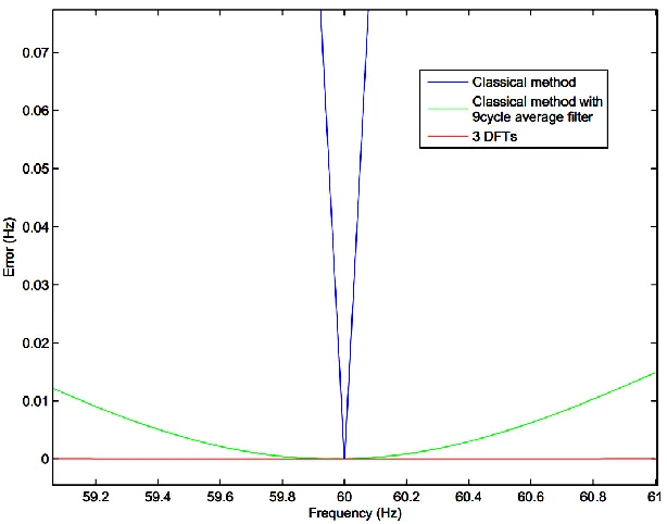
result with selected DFT terms { } { } is shown in Figure 3.1, Figure 3.2 and

Figure 3.3.

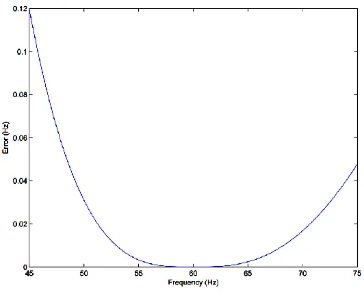
Figure 3.1: Maximum error of different frequency estimation methods

Figure 3.1 is the maximum error of frequency estimated by classical method with a 9

cycle average filter, classical method without filter and the proposed method using three

DFT terms. The result is our proposed method can estimate the frequency very accurately

even though no additional filter is applied. For the frequency range from 59Hz to 61 Hz,

the maximum error is almost zero. For the classical method, an average filter can reduce

the error significantly as discussed in chapter 2.

In Figure 3.2, the maximum error of frequency estimated by the proposed method using

26 0.2 Hz in this range.

Figure 3.3 is the frequency estimate when input signal’s frequency is varying. This can

happen when the power system is transient. Figure shows that the proposed method is

able to estimate the time varying frequency precisely. The error for classical method is

much higher when no filter is used. When an average filter is used to reduce the error, it

still cannot track the frequency accurately because the filter distorts the shape of its input

waveform.

27

28

CHAPTER

4

4.

F

L

P

S

N

I

M

C

O

F

L

P

S

4.1.

The problem of fault location is closely related to power system protection. The

function of protection devices is to isolate the faulted parts from the rest of the system

while the function of fault locator is to find the location of fault accurately. The aim of

both fault location and protection devices is to reduce or prevent damage caused by a

fault, increase the quality of service and reduce overall cost of energy delivery. Fault

locator and protection device both process measurements from instrumental transformers.

Because of these similarities, some commercial protective relays in the market have fault

location function.

When the fault occurs, there will be transient in voltage and current on the faulted line.

Depending on the setting of protective relays, circuit breakers may disconnect the faulted

section. Analyzing an event of fault always need to consider the operation of protection

devices. In [18], the author uses breaker-clearing transient to determine fault location. For

the fault location method that we will discuss in following sections of this chapter,

information from protection devices such as status of circuit breakers (on/off) can assist

the fault location algorithms.

29

four main categories for fault location methods: method using current and voltage

waveforms’ fundamental frequency components, method using current and voltage

waveforms’ high frequency components, method using travelling waves created by fault

and knowledge based methods such as neural networks, fuzzy logics, genetic algorithms,

etc.[8].

In [8], the author described fault location method using measurements of fundamental

frequency current and voltage at one terminal of the line. This method considers circuit

model of line before and during fault to formulate the calculation of distance from fault to

one line terminal. Figure 4.1 is the circuit diagram of faulted line. Using Kirchhoff's law,

the relation between current and voltage measured at terminal A and fault current is:

sA _sB

A B

_line 1 _line

𝐀 𝐁

𝐼_sA

𝐼_A

A

𝐼_sB

𝑅_F

Fault

Figure 4.1: Circuit diagram of faulted line

(4.1)

Fault current distribution factor is defined as:

| |

(4.2)

30

𝐼 𝐼 (4.3)

Substitute (4.3) to (4.1)

𝐼 𝑅 𝐼

| |

(4.4)

(4.4) is equivalent to:

_𝐼

𝐼 𝐼 𝑅 | 𝐼 |

| |

(4.5)

Since 𝑅 | _| |_| is real number, the location of fault is found by taking the imaginary part

of (4.5). Assuming the fault current distribution factor is a real number, fault location can

be determined without knowing source impedances and .

𝐼 𝐼 𝐼

(4.6)

This method is simple and can locate the fault with low resolution measurements.

However, the accuracy of this method decreases when fault current distribution factor is

not a real number. Also, if the fault is clear after a very short time, this method may not

be able to locate fault accurately.

In [17], fault is located by precisely determined the arriving time of voltage or current

travelling waves. Assuming the resistance of transmission line is negligible, voltage and

current are described by partial differential equations:

𝑡

𝑡

𝑡 (4.7)

𝑡

𝑡 𝑡

31

Using the above partial different equations, both voltage are current are derived as

combination of two travelling waves which propagate in opposite directions.

𝑡 (𝑡 ) (𝑡 ) (4.9)

𝑡 [ (𝑡 ) (𝑡 )] (4.10)

where

is the velocity of propagation and √ is the characteristic

impedance or surge impedance.

A F B

t1

t2

1+

1

2 +

2 +

Figure 4.2: Lattice diagram for fault on transmission line

When a fault occurs in a transmission lines, it generates voltage and current transient

waves. From the fault location, these transient waves travel toward two terminals of the

32

transient are illustrated by lattice diagram in Figure 4.2.

The arriving time of transient waves at two terminals are 𝑡 and 𝑡 . Knowing the time

difference, the line’s length and the velocity of wave propagation

, the distance

from fault location to bus A can be determined.

𝑡 (4.11)

High frequency components of voltage and current transients can be used for fault

location. One of the techniques to analyze a transient waveform in frequency domain is

using Fourier transform (4.12).

𝜔

∫ 𝑠 𝑡 𝑡

(4.12)

The author of [18] describes the way voltage waveforms are used to locate fault.

Voltage waveforms at two terminals in a selected time interval that fault occurs are

extracted from original waveforms. The transient components are then obtained by

eliminating the fundamental frequency components (60Hz). After this step is

accomplished, transient waveform are analyzed by Leon Cohen time frequency

distribution. This step can be done by Fourier transform as well. However, time

frequency technique shows a more accurate characterization of transient waveforms.

𝑡 𝜔

∭ 𝑠 ( ) 𝑠 ( )

(4.13)

Transient waveforms of voltages at two terminals of the line have highest magnitudes

at frequencies 𝜔 and 𝜔 . Using (3.13), 𝜔 and 𝜔 can be determined. Location of fault

33

𝜔_𝜔

(4.14)

The limitation of methods using waveforms’ high frequency components or travelling

waves is the requirement of high sampling rate and the availability of communication.

N

I

M

C

4.2.

When a fault happened, network impedance matrix changed. According to [19], the

change that a fault makes in a network can be considered as combination of four basic

cases:

- (1) Add branch from a new bus to ground

- (2) Add a branch connect an existing bus to a new bus

- (3) Add a branch from an existing bus to ground

- (4) Add/remove a branch between two existing buses

When a branch with impedance z is added from a new bus N+1 to ground, the new

network impedance matrix is calculated as:

[

]

(4.15)

When a branch with impedance z is added to connect an existing bus p to a new bus

N+1, the new network impedance matrix is calculated by equation:

[

]

34

When a branch with impedance z is added from an existing bus p to ground, the new

network impedance matrix is calculated by two steps. The first step is to add a branch

with impedance z to a new bus N+1 using the method of case (2). The second step is to

short the new bus N+1 to ground using Kron reduction. New network impedance matrix

has the same size as pre-fault network impedance matrix and is calculated by equations

(4.17) and (4.18).

[

]

(4.17)

(4.18)

Similar to the case (3), calculation of network impedance matrix when a branch with

impedance z is added to connect two existing buses p and q includes two steps. First,

matrix is calculated to represent the new loop. Then Kron reduction was used to

calculate the network impedance matrix of new network.

[

] _(4.19)

(4.20)

Equations (4.19) to (4.20) are calculation of network impedance matrix when a branch

is added to the network but they can also be used when a branch is removed. In that case,

removing a branch with impedance z can be consider as adding a branch with impedance

35

Both open circuit and short circuit event can be calculated using these above basic

cases in combination. Some scenarios will be considered in this section.

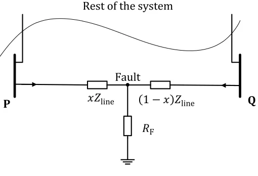
Figure 4.3 is the scenario when three phase fault occurs in transmission line between

bus p and bus q of the network. The distance from fault location to bus p is represented

by variable when fault occurs at bus p and when fault

occurs at bus q. The resistance of fault is 𝑅 .

Before fault occurs, impedance matrix of the system is Z. Impedance of the

transmission line is . The number of nodes is N. The new network during fault

shown in Figure 4.3 can be built by the following steps:

- Remove the branch between two existing buses p and q

- Add a branch with impedance from bus p to new bus N+1

- Add a branch with impedance from bus q to bus N+1

- Add a branch with impedance 𝑅 connecting bus N+1 to ground _{line 1 line}

𝐏 𝐐

Fault

𝑅_F Rest of the system

36

As the result, the network impedance during fault is calculated by the following

equations:

[

]

(4.21)

(4.22)

[

]

(4.23)

[

]

(4.24)

(4.25)

[

𝑅 ]

(4.26)

(4.27)

From (4.21) to (4.27), is the element of impedance matrix at row and

column . is the impedance matrix of faulted system.

Now, we consider the transmission line with two circuit breakers at bus p and bus q. If

37

than the other bus, one circuit breaker will trip before the other. Figure 4.2 shows the

network when the circuit breaker at Q bus trips during fault. The new network impedance

matrix can be built by these steps below:

- Remove the branch between two existing buses p and q

- Add a branch with impedance from bus p to new bus N+1

- Add a branch with impedance connecting bus N+1 to ground

As the result, the network impedance during fault is calculated by the following

equations:

[

]

(4.28)

(4.29)

[

]

(4.30)

[

𝑅 ]

(4.31)

(4.32)

38

For this scenario, the new network impedance matrix can be calculated by simply

removing the branch between bus p and bus q. We will also have the same network for

the case of open fault in transmission line between bus p and q, assuming the line is

inductive and its capacitance can be neglected.

[

]

(4.33)

_{line 1 line}

𝐏 𝐐

Fault

𝑅_F Rest of the system

_{line 1 line}

𝐏 𝐐

Fault

𝑅_F Rest of the system (a)

(b)

Figure 4.4: Faulted system

39

(4.34)

F

F

A

N

-L

L

S

P

4.3.

4.3.1.

L

S

A common problem in engineering is to find parameters of a device or process with

some available measurements. The relation between these parameters that need to be

estimated and the measured variables is known from theoretical study of the object. In

many cases, this problem is over-defined, for example when measurements are taken

multiple times. Least squares method is an approach to solve over-defined equations

where the number of variables is less than the number of equations. Because of the

redundancy, in general case, there is no set of variables that satisfy the system of

equations. Least square method finds the approximate solution that minimizes quadratic

mean of errors made in each equation.

Suppose the relations between unknown variables and measurements are provided as a

set of linear equations:

𝐴 (4.35)

with 𝐴 is a matrix that have more rows than columns, is a matrix with one column,

is the variable. The linear least squares problem is to find solution ̂ to minimize

error ‖ 𝐴 ̂‖.

This is an optimization problem. The solution is

̂ 𝐴 𝐴 _{𝐴 (4.36)}

40

problem that can be solved using least squares. Measurements are taken multiple times at

different points and with each measurement, we have one equation. The set of equations

obtained is: { (4.37)

(4.37) can be expressed in the matrix form (4.35) with

𝐴 [ ] [ _] [ ] (4.38) Figure 4.5: Data fitting using linear least square

0 0.5 1 1.5 2 2.5 3

41

̂ 𝐴 𝐴 _{𝐴 [}

] (4.39)

That means the line in Figure 4.5 is .

4.3.2.N

-

L

S

When the relation between unknown variables and measurements is non-linear,

equation has the form:

(4.40)

Similar to the case of linear least square, solution ̂ has to minimize quadratic mean

error ‖ ̂ ‖.

Figure 4.6: Solving non-linear equations

As a non-linear equation, (4.40) can be solved using iteration. However, because it is

redundant, each steps of the iteration is solved using linear least square. The iteration

process is described in Figure 4.6.

0 1 2 3 4 5

-10 0 10 20 30 40 50

x0

42

The iteration starts at . If variable is has one dimension only, the equation of

tangent line is:

|

(4.41)

Then the first step of the iteration is to find where tangent line (4.41) cuts horizontal

axis ( ).

|

(4.42)

Equation (4.42) can be solved by linear least square method (4.36):

_(4.43)

with

| . When has more than one dimension , H is a

matrix of first partial derivatives of function :

[ |

_|

_| ]

(4.44)

Notice that function may have more than one dimension so matrix H can have more

than one row.

For example, for the equation

[

] [ ]

(4.45)

43

[

]_|

(4.46)

After the solution of (4.43) is found then assign and repeat the process until

the incremental error is small enough ‖ ‖ .

4.3.3.

F

F

L

Consider the location of fault and fault resistance are unknown

variables, the network impedance matrix during fault can be calculated as a function of

by equations (4.21) to (4.27). Then the voltages at all nodes in the network can

be calculated as a function of as well:

[ ] [ 𝐼 𝐼

𝐼

] _(4.47)

with 𝐼 is current injected to bus i.

Currents at all lines in the network then can be calculated from bus voltages and line

impedance data. As a result both bus voltages and line currents 𝐼 can be calculated as

function of :

𝑅 (4.48)

𝐼 𝑅 (4.49)

Consider the network that we have voltage phasor measurements at buses

and current phasor measurement at lines

44

[

𝑅 𝑅

𝑅 𝑅 𝑅

𝑅 _] [ 𝐼 𝐼

𝐼 ]

(4.50)

(4.50) is the set of m+n equation with 2 variables. Using non-linear least square

45

CHAPTER 5

5.

T

C

PSCAD

R

In this chapter, fault location method described in chapter 4 is applied to locate fault in

three test cases: 6 bus network case, single circuit line case and double circuit lines case.

For the 6 bus network case, the fault locator uses model of the of the system and

measurement data obtained from simulation. For the single circuit line case and double

circuit lines case, the system model is estimated from voltage and current measurements,

then this model is used to locate fault. All three test cases are simulated in PSCAD.

6

B

N

C

5.1.

5.1.1.

S

D

The 6 bus system in has two voltage sources and four loads at bus 2, 3, 4 and 5.

Voltage level is 169 kV. Pre-fault system is described in Table 5.1,

Table 5.2 and Table 5.3 . As the length of transmission line is short, line capacitance is

neglected in this test case.

The simulated scenario is a three phase ground fault. Fault occurs in transmission line

that connects bus 4 and bus 5. Location of fault is 125 km from bus 4 which is equal to

85% of total length of the line. The duration of fault is 0.5 s and after fault is clear, the

system is back to normal operation. The fault resistance is 50 Ohm.

46

doesn’t change during the fault. Instantaneous voltages of bus 1 and bus 5 and

instantaneous currents of line 1-2 and line 5-3 are measured.

BUS 1 BUS 2 BUS 3 BUS 5 BUS 6

BUS 4

30 km 75 km 90 km 30 km

100 km 150 km

Figure 5.1: 6 bus system

Table 5.1: Voltage sources in 6 bus system

Voltage source at bus Magnitude

(kV)

Angle (Degree)

1 164.22 1.91

6 164.22 0

Table 5.2: Load in 6 bus system

Load at bus

Real power (MW)

Reactive power (MVAR)

2 20 4

3 100 5

4 10 30

47

Table 5.3: Line parameters

Line Length (km) Resistance

(Ohm)

Inductance (Ohm)

1-2 30 1.5864 12.887

2-3 75 3.9659 32.2175

2-4 100 5.2879 42.9567

3-5 90 4.7591 38.6610

4-5 150 7.9318 64.4351

5-6 30 1.5864 12.8870

5.1.2.

R

The three phase ground fault described in section 5.1.1 is simulated in PSCAD. Three

phase instantaneous voltages and currents are measured and imported to MATLAB.

Figure 5.2 is a close look of instantaneous current in line 1 – 2 at the moment fault

occurs. The increase of current magnitude indicates that the fault is fed from power

source at bus 1.

After instantaneous voltages and currents from PSCAD are imported to MATLAB,

they will be processed by the phasor measurement algorithm mentioned in chapter 2.

Positive sequence voltage and current phasors are estimated. Because a phasor has

complex value, we will have phasor magnitude and phase angle. These magnitude and

phase angle of our selected voltage and current change as the fault occurs.

Figure 5.3 and Figure 5.4 show that there are both changes in current magnitude and

48

Voltage at bus 1 doesn’t change because the power source used in this simulation is ideal.

Figure 5.2: Instantaneous current in line 1 – 2

This observation shows that current phasor is more sensitive to fault and it will be

useful to use current magnitude, current phase angle or both of them to detect the fault.

Certainly, for the case fault impedance is high, the change of current magnitude and

phase angle will be small and as a result, a specified detection method for high

impedance fault detection will need to be used. This issue however is not covered in the

scope of this thesis.

In Figure 5.3 and Figure 5.4, red dots indicate the selected moment which faulted line

is connecting to ground through a resistance. In this case, the moment is 𝑡 s. 𝑡 is

selected so that the system has reached steady state and both circuit breakers are closed.

The fault locator can select this moment by looking at the change in magnitude and phase

angle of current phasors. Also, the state of circuit breakers can be used to improve the

accuracy of the fault location algorithm if there is communication between circuit

breakers and the operation center.

0.94 0.96 0.98 1 1.02 1.04

-2 -1.5 -1 -0.5 0 0.5 1 1.5 2

I12 magnitude

kA

Time (s) Ia

49

Figure 5.3: Voltage and current phasors at bus 1

Figure 5.4: Voltage and current phasors at bus 5

In practice, it can happen that two circuit breakers at two ends of the faulted line trips

quickly after the moment fault occur. From chapter 2, we have concluded that the phasor 0 0.5 1 1.5 2

0 50 100

V1 magnitude

kV

0 0.5 1 1.5 2 0 0.5 1 1.5 I12magnitude kA

0 0.5 1 1.5 2 -6

-4 -2 0 2x 10

-3 _{V1 angle}

Time (s)

ra

d

ia

n

0 0.5 1 1.5 2 -0.45 -0.4 -0.35 -0.3 -0.25 I12 angle Time (s) ra d ia n

0 0.5 1 1.5 2 0

50 100

V5 magnitude

kV

0 0.5 1 1.5 2 0 0.2 0.4 0.6 0.8 I53 magnitude kA

0 0.5 1 1.5 2 -0.25 -0.2 -0.15 -0.1 -0.05 V5 angle Time (s) ra d ia n

50

estimation is reliable only when the data window of the signal is in steady state. Hence, if

the circuit breakers trips before 1 cycle of steady state voltage and current waveforms are

collected, the estimation will not be accurate. In this case, transient monitoring function

can be used to in the selection of 𝑡 .

At moment 𝑡 we have measured value of voltages at bus 1 and bus 5 and currents in

line 1 – 2 and line 5 – 3 𝐼 𝐼 . From (4.48) (4.49) and (4.50), these values can

be calculated from system’s model as a function of fault location and fault resistance,

with assumption that fault occurs on a particular line:

𝑅 (5.1)

𝐼 𝑅 (5.2)

The equation with variable and 𝑅

[

𝑅 𝑅 𝑅 𝑅 ]

[_𝐼 𝐼

] _(5.3)

Table 5.4 is the solutions for fault location and fault resistance.

In Table 5.4, N/A means the iteration process to solve (5.3) doesn’t converge or the

solution found is out of boundary. The constraints for fault location and fault resistance

are and 𝑅 . E is the absolute value of the left side of equation (5.3).

With assumption that fault occurs on line 3-5, the iteration process converses to the

point and 𝑅 46 Ohm. Suppose fault occurs on line 3-5, the iteration

process converses to the point and 𝑅 46.4 Ohm. Now, the error E is

51

answer because it minimizes the absolute value of the left side of equation (5.3).

Table 5.4: Fault location and fault resistance

Assume fault occurs on line

Fault location (%)

Fault Resistance

(Ohm)

Error

1-2 N/A N/A

2-3 N/A N/A

2-4 N/A N/A

3-5 80.96 46 2.8551

4-5 85.6 46.4 0.8779

5-6 N/A N/A

Table 5.5: 6 bus system fault location result

Faulted line Location of fault

Error in percentage of line length

1-2 85.6 % 0.4 %

S

C

L

C

5.2.

Single circuit line is the simplest case of the fault location problem. Now, the fault

locator receives available measurements from this line and uses these data to detect if

fault occurs and the location of fault on this line. The system consists of the line that fault

locator is monitoring and the outside network. The impedance of the line can be

estimated from the line length and cable type. The outside network is unknown.

52 system with an extra link line.

Figure 5.5 is the equivalent model of the single circuit line case. The two terminals of

the monitored line are name A and B. The equivalent network consists of two ideal

voltage sources and and two source impedance and . The extra link line

with impedance represents the flow of current from bus A to bus B through the

outside network. When , the system becomes two-machine system. In many

applications, these values of source impedance are provided for the most typical

operations of the system [8]. However, in modern power system with high penetration of

distributed power generations and load fluctuations, the provided data may not be

accurate. In section 5.2.2, method to obtain the parameters of equivalent model will be

discussed.

5.2.1.

S

D

The single circuit line case is simulated in PSCAD and simulation data is imported to

Matlab for processing. The system consists of voltage sources and impedances listed in

Table 5.6.

sA _sB

A B

_line 1 _line

E

𝐀 𝐁

𝐼_sA

𝐼_A

A B

𝐼_sB 𝐼_sE

Fault