Linking speech enhancement and error concealment based on recursive MMSE estimation

R E S E A R C H

Open Access

Linking speech enhancement and error

concealment based on recursive MMSE

estimation

Balázs Fodor

, Florian Pflug and Tim Fingscheidt

Abstract

Speech enhancement and error concealment have seen a considerable progress over the past decades. Although both fields deal with distorted speech signals, there has rarely been an attempt to relate respective approaches to each other. In this paper, for the first time, a clear synopsis of recursive minimum mean square error (MMSE)

estimation in both fields is provided. Our work intentionally does not propose a certain algorithm furthering the state of the art, nor does it provide simulation results of algorithms. Instead, our aim is threefold: First we revisit the basics of Bayes estimation in a recursive manner, covering both kinds of distortion acoustic noise as well as transmission channel noise. Second, we present recursive MMSE estimation applied to speech enhancement (in the frequency domain, as typical) and applied to error concealment (in the time domain, as typical) in strictly coherent notations and provide respective overview diagrams. Finally, we discuss commonalities and differences between both approaches, identify a particular strength of error concealment in general, and provide possible research directions for speech enhancement. A particularly interesting observation is that noise introduced by error concealment is far from being Gaussian and that additive acoustic noise can be expressed in terms of bit errors in DFT coefficients providing a potential interface to error concealment approaches.

Keywords: MMSE estimation; Speech enhancement; Error concealment

1 Introduction

Minimum mean square error (MMSE) estimation is omnipresent in a wide range of research fields and appli-cations. It belongs to the family of Bayesian estimators which are based on the following model: The unobserv-able quantity to be estimated is considered to be the outcome of a random process such as a speech sam-ple [1,2]. These outcomes can be measured through a channel introducing distortions, resulting in so-called observations. Besides the observations, Bayes estimators usea prioriknowledge about the aforementioned random process and the channel, resulting in improved estimation results [2].

Based on this model, MMSE estimators minimize the estimation error variance conditioned on the observa-tions. As an example, the widely used Wiener filter is

*Correspondence: [email protected]

Technische Universität Braunschweig, Institute for Communications Technology, Schleinitzstr. 22, 38106, Braunschweig, Germany

optimal with respect to the MMSE error criterion [2]. In speech enhancement, it is widely assumed that the observations are statistically independent of each other, therefore, MMSE estimation of speech is carried out sequentially by means of the current observation only [3]. Signal history, such as the last speech estimate, is merely used for smoothing purposes in a practical system (cf. [3], Section V). Assuming, however, a dynamic signal model in the form of an autoregressive (AR) speech process, e. g., in conjunction with the source-filter model [4,5], the optimal MMSE estimator is able to exploit signal redundancy by employing both the current and previous observations [6]. In this case, under certain assumptions, the estimation can be carried outrecursivelyand can be split into two steps typically decreasing computational complexity and relaxing memory requirements [7]. The first step exploits signal history in the form of previous observations providing ana prioriestimate which is sub-sequently corrected in a second step taking into account

also the current observation, resulting in ana posteriori estimate.

In speech enhancement, the following model is widely employed for MMSE estimation: The unobservable speech is distorted by the unobservable acoustic noise, resulting in the observations in the form of noisy speech. The aim of speech enhancement is to estimate the speech by means of some a priori knowledge and the obser-vations. State-of-the-art speech enhancement is often carried out in the short-time Fourier transform (STFT) domain and it is assumed that the discrete Fourier transform (DFT) coefficients of the speech and the acoustic noise are statistically independent. Thus, the

a priori knowledge employed for MMSE estimation is

a specific distribution of the speech (Gaussian [3,8,9], super-Gaussian [10-12]) and the acoustic noise (typi-cally Gaussian). Classical MMSE estimators for speech enhancement under a Gaussian speech assumption are, e. g., the Wiener filter (e. g., [13]), the MMSE short-time speech amplitude (STSA) estimator [3], or the MMSE log-spectral amplitude (LSA) estimator [9]. These estimators mainly differ with respect to the estimation domain, i. e., instead of the complex-valued DFT coefficients, an arbi-trary function of it is estimated (typically its amplitude or the logarithm of its amplitude).

In speech enhancement, the widely used Kalman fil-ter [6] can be employed as arecursiveMMSE estimator. In Kalman filtering, a Gaussian assumption is made for the acoustic noise and the error of the a priori speech estimate. In [14], a Kalman filter was proposed for time-domain speech enhancement. The proposed approach models the speech as an AR process based on a predictor, therefore, the estimation employs the current and the pre-vious observations and, according to Kalman theory, the estimation of the speech is carried out recursively in two steps. A DFT-domain Kalman filter for speech enhance-ment was introduced, e. g., in [15-17]. In [15], the Kalman filter operates on complex-valued DFT coefficients and the speech was modeled as an AR process, while the noise process was assumed to be memoryless. In [16], differ-ent approaches to calculate the prediction coefficidiffer-ents and different estimators for calculating thea posteriorispeech were investigated. Additionally, the memoryless assump-tion for the noise was replaced by an AR noise model in [17].

In error concealment, the following model is widely utilized: On the transmitter side, speech samples or source-coded parameters are quantized and mapped to corresponding bit combinations. These are transmitted over digital error-prone transmission channels and are received as bit-wise log-likelihood ratios (LLRs) compris-ing channel reliability information by the decoder. The aim of error concealment is the disguise of transmission errors which would otherwise lead to an unacceptable

degradation of speech quality on the receiver side. This is achieved by MMSE estimation of unobserv-able speech samples or source-coded parameters, requir-ing a posteriori probabilities. These are proportional to both a likelihood term resulting from the received LLRs and a prior term comprising the available inher-ent signal redundancy as a prioriknowledge at decod-ing time. This approach has been employed for robust source decoding of speech signals [18-23], source-coded audio signals [24,25], and uncompressed audio [26] that exploit signal redundancy in sample values or various source codec parameters (e. g., scaling factors, line spec-tral frequencies (LSFs) vectors, vector-quantized gains, adaptive codebook indices). Thereby, the signal redun-dancy is exploited by a time-variant modeling of the prior either using Markov chains [18-24] or employ-ing approaches based on linear prediction in [25,26]. Typical applications are speech and audio transmis-sion systems such as mobile phones or digital wireless microphones.

The aim of this paper is to reveal links between the fields of speech enhancement and error concealment focusing on recursive MMSE estimation approaches. We will show that the main structure of recursive MMSE estimation is the same in both disciplines which allows for draw-ing interestdraw-ing links between tackldraw-ing acoustic noise and transmission channel noise. In speech enhancement, the well-known Kalman filter can be employed as optimal recursive MMSE estimator which assumes that the acous-tic noise is Gaussian distributed. Transmission channel noise as found in distorted speech signals, however, is far from a Gaussian distribution and — motivated by the nature of digital transmission — is rather modeled on bit level in error concealment which allows for exploit-ing powerful bit reliability information. This extraa pri-ori knowledge can be identified as a definite strength of error concealment compared to speech enhancement. Based on this finding, this paper sketches as outlook new research directions for speech enhancement exploiting bit likelihoods.

2 On recursive MMSE estimation

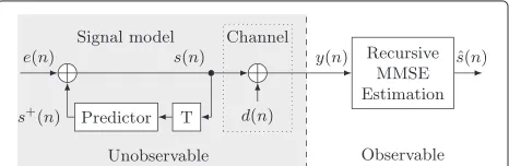
As pointed out in Section 1, the aim of recursive MMSE estimation is to estimate the unobservable speech sam-pless(n), withnbeing the discrete time index, which are transmitted through either an acoustic or a transmission channel. This channel distorts the speech signal by super-imposing unobservable noise samples d(n) being mod-eled as statistically independent, resulting in the observed noisy speech signal (cf. Figure 1)a

y(n)=s(n)+d(n). (1)

The estimation of the clean speech s(n) is carried out by means of all previous and the current observations

yn₀ = y(0),y(1),. . .,y(n−1),y(n)T, with (·)T denoting the transpose operation, as well as by somea priori knowl-edge about the speech signal and the channel, resulting in the clean speech estimateˆs(n)(cf. Figure 1).

The a priori knowledge about the speech includes

the following autoregressive model [14]: The current speech sample s(n) is assumed to be a sum of the predicted speech s+(n) and the prediction error e(n) (cf. Figure 1), the latter being a zero-mean (random) signal which is statistically independent ofs+(n). The pre-dicted speech is generated by a predictor of the order Np ass+(n) = aT · snn−−1Np with s

being the so-called prediction coefficients. Please note that these coefficients are time-variant in practice, there-fore, they need to be estimated. However, assuming a slow time variability,ais treated as a constant for the moment. According to the speech signal model, the current speech samples(n)is statistically dependent not only on the current observation y(n) but also on the previous onesyn₀−1, thus, these are also included in the estimation process [6]. This paper deals with recursive estimation, therefore, the estimation process is typically split into two parts, namely thepropagationstep and the updatestep. The propagation step exploits the previous observations to provide ana prioriestimate of the current speech sam-ple s(n). Since this estimate can yield a relatively high error variance, the update step improves it incorporating the current observationy(n), resulting in thea posteriori

Figure 1Signal model, channel, and recursive MMSE estimation.

speech estimateˆs(n). Hence, the information carried by the previous observations becomes successively part of thea prioriknowledge during the estimation process.

2.1 The estimator

The recursive MMSE estimation with the underlying sig-nal model as in Figure 1 yields

ˆ

with E{·} being the expectation operator, p(·) being a probability density function (pdf ), and p(s(n)|y(n),y₀n−1) = ps(n)|yn₀being the so-called pos-terior. Usually, the posterior is computed by means of Bayes’ rule, therefore, (2) can be rewritten as

ˆ

likelihood, the prior, and the evidence, respectively. Please note that the evidence is typically calculated by marginal-izing the pdf product of the numerator in (3).

2.2 The prior

As can be seen above, the prior is a function of the previous observationsyn₀−1. However, the prior can also be determined recursively by marginalization using the signal model in Figure 1 as

ps(n)yn₀−1 =

The first pdf in the integral is a predictor pdf, the second one is the joint pdf of the lastNpposteriors. Therefore, the current prior is obviously dependent on the (distribution of the) lastNpestimates. Moreover, the mean of the prior using the signal model in Figure 1 turns out to be

Es(n)yn₀−1

innovation, e. g., [7]) is orthogonal to the previous speech samples and, therefore, also to the previous observations (e. g., [7,27]). Thus, we obtainE{e(n)|y₀n−1} =E{e(n)} =0. Assuming that this a priori speech estimate ˆs+(n) = fyn₀−1 is a sufficient statistic fors(n), the prior turns out to be

p(s(n)|yn₀−1)=p(s(n)|ˆs+(n)). (6)

This pdf describes the clean speech given the a priori speech estimate, in other words, it is the pdf of the prop-agation errore¯(n) = s(n)− ˆs+(n)which can be written as

ps(n)ˆs+(n)=p¯e

¯

e(n)=s(n)− ˆs+(n). (7)

Using the signal model in Figure 1, the variance of the propagation error turns out to be [28]

E{(s(n)− ˆs+(n))2} =E{e2(n)} +E{(s+(n)− ˆs+(n))2} =σ2

e(n)+σe2+(n)=σ¯e2(n) (8)

withσ_e2(n) = Ee2(n)being the prediction error vari-ance andσ_e2+(n)=E

s+(n)− ˆs+(n)2. Please note that (8) holds independently of the type of the propagation error pdf.

2.3 The likelihood

Thea prioriknowledge about the (acoustic or transmis-sion) channel is contained in the likelihood. This means that the additive noise d(n), which distorts the clean speech s(n) (cf. Figure 1), is modeled by the likelihood py(n)s,yn₀−1 . Assuming a memoryless (acoustic or transmission) channel, meaning that the noise samples d(n), d(n −1),. . . are statistically independent of each other, the likelihood is [29]

p(y(n)|s(n),y₀n−1)=p(y(n)|s(n)) (9)

being the pdf ofy(n)given a specific speech samples(n). Therefore, this is the pdf of the additive noise d(n) = y(n)−s(n)as [3]

py(n)|s(n)=p_dd(n)=y(n)−s(n). (10)

Since the variance of the noiseσ_d2(n)=Ed2(n)cannot be measured directly in practice, it is usually estimated by a noise power estimator or a channel quality estimator.

3 Application to speech enhancement

Assuming that the speech and the noise processes are at least quasi-stationary along the time frames in each frequency bin k and statistically independent of each other, the signal model in Figure 1 is also valid in the STFT domain. Accordingly, the aim of recursive

MMSE estimation in speech enhancement is to esti-mate the clean speech DFT coefficients S(k) which are generated by an autoregressive process as sketched in Section 2: The clean speech S(k) is modeled by the sum of the predicted speech S+(k) and a statisti-cally independent, zero-mean prediction errorE(k), i. e., S(k) = S+(k) + E(k). S+(k) is calculated by a pre-dictor of the order Lp as S+(k) = AH(k) · S−₋1_Lp(k)

with A(k) = ALp(k),ALp−1(k),. . .,A1(k) T

being the complex-valued prediction coefficients and S−₋1_L

p(k) =

S−Lp(k),S−Lp+1(k),. . .,S−1(k) T

. It is assumed that the prediction coefficients change very slowly along the frames and are, therefore, modeled as constants for the moment. The acoustic channel distorts the speech spectrum by superimposing some statistically indepen-dent acoustic noiseD(k), so thatY(k) =S(k)+D(k) withY(k)being the noisy speech DFT coefficients. The estimated speech DFT coefficientsS(k)are calculated by the recursive MMSE estimator employing the underlying observationsY₀(k)=[Y0(k),Y1(k),. . .,Y(k)]Tas (cf. (2))

S(k)=ES(k)Y(k),Y₀−1(k). (11)

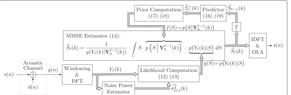
A block diagram of recursive MMSE estimation for speech enhancement assuming a memoryless acoustic channel is given in Figure 2. Please note that the upper signal path is related to the prior computation, the block in the cen-ter is the MMSE estimator (11), and the lower signal path refers to the likelihood computation. Starting in the lower left-hand corner, windowed segments of the noisy speech signaly(n) = s(n)+d(n)are transformed into the DFT domain, followed by the likelihood computation.

3.1 The likelihood

Since a memoryless acoustic channel is assumed, the likelihood turns out to be (cf. (9) and (10))

p

Y(k)S(k),Y₀−1(k) =pY(k)|S(k) =pD

D(k)=Y(k)−S(k). (12)

As can be seen, the likelihood is a function of the noisy speech (cf. Figure 2). Moreover, after computing the like-lihood by means of the current observation Y(k), the likelihood remains a functiong(S)of the unknown speech DFT coefficientS(cf. output of ‘Likelihood Computation’ in Figure 2). Furthermore, as we will see later,Swill be the integration variable of the MMSE estimator (cf. (11)).

Figure 2STFT domain recursive MMSE estimation for speech enhancement assuming a memoryless acoustic channel.

p(Y(k)|S(k))= 1 πσ2

D,(k)·

exp

−|Y(k)−S(k)|2

σ2

D,(k)

(13)

with σ_D2_,(k) being the variance of the quasi-stationary noise processD. Please note that also for non-Gaussian noise pdfs, the likelihood is always a function of the noise powerσ_D2_,(k)(cf. connection between ‘Noise Power Estimator’ and ‘Likelihood Computation’ in Figure 2). Therefore, in practice, its estimate σ_D2_,(k) is calculated by a noise power estimator using the noisy speech DFT coefficients [30-32].

3.2 The estimator

Using the likelihood (12), the clean speech DFT coeffi-cientsS(k)are estimated as (cf. (2), (3), and (11))

S(k)=

C

S·p(S|Y₀−1(k))·p(Y(k)|S)dS

p(Y(k)|Y₀−1(k)) (14)

with the evidence

p(Y(k)|Y₀−1(k))=

C

p(S|Y₀−1(k))·p(Y(k)|S)dS

(15)

and the priorp

SY₀−1(k) . Please note that both the prior and the likelihood are a function of the integration variableS, namelyf(S)(cf. upper signal path in Figure 2) andg(S)(cf. lower signal path in Figure 2), respectively. The estimated clean speech signal ˆs(n) is obtained by taking the inverse DFT (IDFT) ofS(k) from (14) and performing, e. g., an overlap-add (OLA) step.

3.3 The prior

As discussed in Section 2, thea priorispeech estimate is calculated as (cf. (5))

S+(k)=AH(k)·S−₋1_Lp(k). (16)

This step is denoted as ‘Predictor’ in the upper signal path in Figure 2. Please note that the predictor employs previous speech estimates which is reflected by the delay unit denoted by ‘T’ in Figure 2. Assuming that thea pri-orispeech estimateS+(k) is a sufficient statistic for the speech S(k), the prior turns out to be the pdf of the propagation errorE¯(k)=S(k)−S+(k)(cf. (6) and (7))

p(S(k)|Y₀−1(k))=p_E¯(E¯(k)=S(k)−S+(k)). (17)

Employing a specifica priorispeech estimateS+(k), the prior remains a function of the speechf(S) and can be fed into the MMSE estimator (14) (cf. connection between ‘Prior Computation’ and ‘MMSE Estimator’ in Figure 2).

Assuming that the (complex-valued) propagation error is a zero-mean Gaussian process with i. i. d. real and imag-inary parts, the prior is calculated [15,16]

pE¯

_¯

E(k)= 1

πσ2 ¯

E,(k) ·exp

−| ¯E(k)|2 σ2

¯

E,(k)

(18)

withσ2_¯

E,(k) being the propagation error variance which cannot be measured in practice, thus, it has to be esti-mated [15,16].

Since the prediction coefficients A(k) in (16) are not accessible in practice, they need to be estimated as well, e. g., by the widely used normalized least-mean-squares (NLMS) algorithm [7]. Introducing again time variabil-ity, the prediction coefficients for the next frame are calculated recursively as

A+1(k)=A(k)+μ·

E∗(k) ||S−₋1_L

p(k)||

2₊·S −1

−Lp(k) (19)

3.4 The Kalman filter

The estimator (14) requires calculating two integrals over the whole complex plane for each time-frequency unit (,k). Fortunately, this estimator can be obtained in closed form by solving these integrals, reducing the computational complexity for practical implementations. Assuming a Gaussian distribution for both the propaga-tion error (18) and the acoustic noise (13), the MMSE estimator (14) turns out to be a sum of thea priori esti-mate and the update (the derivation can be found in the Appendix) in the form of the Kalman filter equations (cf. [15], Equation 12)

S(k)=S+(k)+E(k) (20)

with

E(k)=K(k)·R(k), (21)

K(k)= ζ(k)

1+ζ(k), (22)

R(k)=Y(k)−S+(k) (23)

where K(k) is the so-called Kalman gain and ζ(k) =

σ2 ¯

E,(k)/σD2,(k)(cf. thea prioriSNR in [3]). The latter can be estimated by [16]

ˆ

ζ(k)=β|E−1(k)|

2

σ2

D,−1(k)

+(1−β)max ⎧ ⎨ ⎩

|R(k)|2 σ2

D,−1(k)

−1, 0 ⎫ ⎬ ⎭ (24)

withβbeing a smoothing factor, typically chosen close to one.

Please note that the recursive nature of MMSE esti-mation is well reflected by (20): The a priori estimate S+(k)utilizing the previous observations is corrected by the termE(k)employing the current observationY(k), resulting in thea posteriorispeech estimateS(k).

4 Application to error concealment

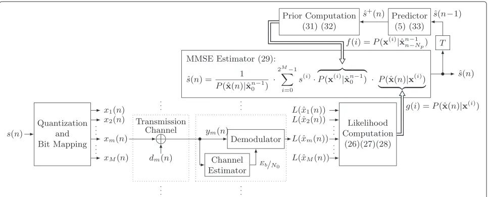
The aim of error concealment is to estimate transmitter-sided (speech) samples, e. g., by a recursive MMSE esti-mator, in order to conceal distortions due to residual bit errors after demodulation or channel decoding. Bit error concealment of PCM audio or speech could the-oretically be carried out by the equations in Section 2 using the hard-decoded receiver-sided samples. However, in order to exploit more information for improved esti-mation results, it is often advantageous to employ error concealment using reliability information on a bit level as in [19,26]. A block diagram of such a soft-decision decod-ing scheme based on recursive MMSE estimation is given in Figure 3. Similar to Figure 2, the likelihood compu-tation is related to the lower signal path, the estimator can be found in the center, and the prior computation is performed in the upper signal path.

4.1 The likelihood

In error concealment, it is assumed that each transmitter-sided sample s(n), being processed as introduced in Section 2, is quantized with M bit and, therefore, can bijectively be mapped to a natural-binary bit combina-tionx(n) = [x0(n),x1(n), . . .,xm(n),. . .,xM−1(n)] (see ‘Quantization and Bit Mapping’ in Figure 3). Assum-ing further binary phase-shift keyAssum-ing (BPSK) modulation, each transmitted bit (BPSK symbol) xm(n) ∈ {−1, 1} is more or less distorted by the channel, modeled by the real-valued channel noise dm(n) (cf. ‘Transmission Channel’ in Figure 3). For the demodulation of the received real-valued noisy symbols ym(n), the so-called energy per bit to noise power spectral density ratioEb/N0 is needed which is calculated by the channel estimator (cf. connection between ‘Channel Estimator’ and ‘Demodula-tor’ in Figure 3). The demodulator then calculates the LLR which is defined as

L(xˆm(n))=ln

P(xˆm(n)|xm(n)= +1) P(xˆm(n)|xm(n)= −1)

(25)

with the hard-decided receiver-sided bit xˆm(n) = sign(ym(n))representing the receiver-sided observation. In practice, the LLR is calculated by means of E_b/N0 and ym(n) (cf. the two inputs of the ‘Demodulator’ in Figure 3)bwhich reflects the likelihood of a possibly trans-mitted bit xm(n). The bit-error probabilities BERm(n) describe the probability that a transmitted bit was dis-torted through the channel and can be calculated by means of the LLRs as [33]

BERm(n)= 1

1+e|L(xˆm(n))|. (26)

Once each transmitter-sided samples(n) is quantized, it assumes a discrete values(i) with i ∈ {0, 1,. . ., 2M−1}. Moreover, eachs(i)can be mapped to one corresponding bit combinationx(i). The bit-wise transition probabilities define thebitlikelihood given bitx(mi)of theith quantiza-tion table entry [19]

P

ˆ

xm(n)x(mi) =

BERm(n), ifxˆm(n)=x(mi), 1−BERm(n), else.

(27)

Assuming that the transmission channel is memoryless and that the bit distortions dm(n) are statistically inde-pendent of each other along the bit indicesm, thesample likelihood is computed as (cf. ‘Likelihood Computation’ in Figure 3 and, e. g., [19])

Pxˆ(n)x(i) =

M−1

m=0

Pxˆm(n)x(mi) . (28)

Figure 3Time domain recursive MMSE estimation for error concealment assuming a memoryless transmission channel.

likelihood (28) and for any further processing, however, the estimator deals with samples again.

4.2 The estimator

The recursive MMSE estimator (3) turns out to be a sum

ˆ s(n)=

2M_!−1

i=0

s(i)·P(x(i)|ˆx₀n−1)·P(xˆ(n)|x(i))

P(xˆ(n)|ˆxn₀−1) (29)

with the evidence

Pxˆ(n)xˆn₀−1 = 2M₋₁

"

i=0

Px(i)xˆn₀−1 ·Pxˆ(n)x(i) , (30)

the samplelikelihood (28), and the prior Px(i)ˆxn₀−1 . Please note that both the prior and thesamplelikelihood are a function of the summation indexi in (29), namely f(i)(cf. upper signal path in Figure 3) andg(i)(cf. lower signal path in Figure 3), respectively. The result of the summation is the speech estimatesˆ(n)(cf. right-hand side of the MMSE estimator in Figure 3).

4.3 The prior

As discussed in Section 2, thea priorispeech estimate is calculated as ˆs+(n) = aT · ˆsn_n−₋1_Np = f

ˆ

xn₀−1 (cf. (5)). This step is carried out in the block ‘Predictor’ in Figure 3. Just as in Section 3, the predictor incorporates the pre-viously estimated speech samples, reflected by the delay unit ‘T’ in Figure 3. Assuming that thea priorispeech esti-matesˆ+(n) is a sufficient statistic fors(i) and using that each bit combinationx(i)can bijectively be mapped to one correspondings(i), the prior turns out to be

P

x(i)ˆxn₀−1 =P

s(i)ˆs+(n) . (31)

However, sinces(i)is a quantized quantity, the probabil-ity of itsith value can be calculated as [34]

P(s(i)|ˆs+(n))=

Ii

pe¯(s− ˆs+(n))ds (32)

withpe_¯(·) being the propagation error pdf and with the PCM sample quantization intervalsIi,i=0, 1,. . ., 2M−1. Employing a specifica priorispeech estimatesˆ+(n), the prior remains a function of summation indexiasf(i)and can be fed into the MMSE estimator (29) (cf. connection between ‘Prior Computation’ and ‘MMSE Estimator’ in Figure 3).

Please note that in [26], the quantity E s+(n)−

ˆ s+(n)2

in (8) was assumed to be zero. Furthermore, assuming that the prediction errore(n)=s(n)−s+(n)is stationary, the propagation error pdf can be determined by a histogram measurement in a training process. More-over, online integration ofpe_¯(·)is not necessary if the inte-grations overIi intervals are performed beforehand and ˆ

s+(n)is quantized withMbits, leading to discrete prob-abilitiesP¯e(·)[26]. Thus, employing a lookup table con-taining the precomputed P¯e(·)values in the block ‘Prior Computation’ in Figure 3, the table entries can be indexed by the quantizeda priorispeech estimateˆs+(i)(n). Hence, the resulting priorP(s(i)sˆ+(i)(n))being a function of the summation indexican be obtained in a computationally efficient way.

ˆ

a(n+1)= ˆa(n)+μ· eˆ(n) ||ˆsn_n−₋1_Np||2₊· ˆs

n−1

n−Np (33)

witheˆ(n) = ˆs(n)− ˆs+(n) as well as withμandbeing the step size constant and the regularization parameter, respectively. Please note that the prediction coefficients can alternatively be obtained by a slightly modified NLMS algorithm [26,35].

5 Links between speech enhancement and error

concealment

So far, we have introduced an application example of recursive MMSE estimation for both speech enhancement and error concealment. In this section, we aim at showing links between the presented estimators.

As can be seen above, while the estimator (14) used for speech enhancement (cf. Figure 2) utilizes continuous distributions, the estimator (29) employed for error con-cealment deals with discrete ones (cf. Figure 3). In error concealment, the samples of the signal to be transmitted are quantized typically by 16 bit or 24 bit and thus are from a finite set of elements, whereas in speech enhance-ment the digital signals are assumed to be quantized fine enough (even though quantization with 64, 32, or 16 bit may take place), therefore, the codomain of the samples is assumed to becontinuous.

5.1 The likelihood

This also influences the channel model. While in speech enhancement, the noise is modeled on asample(or coeffi-cient) level (1), in digital transmission and error conceal-ment the noise occurs on a modulation symbol level or, for BPSK equivalently, on bit level (26), (27): The transmitted binary source bits (BPSK: symbols)xm(n)are distorted by the real-valued channel noisedm(n). Using the received value (symbol) ym(n), the demodulator calculates a cor-responding LLRL(xˆm(n))by means ofEb/N0, which is a normalized SNR measure being a function of the channel noise power. Therefore, the likelihood (28) being com-puted by means of the LLRs (cf. (26), (27), and (28)) is a function of the channel noise power as it is the case in speech enhancement (cf. (13)). Thus, in both speech enhancement and error concealment, the current obser-vation (Y(k)orym(n)) and the channel noise power (den-sity) (σ_D2_,(k)orN0) are needed for likelihood computation (cf. Figures 2 and 3).

However, there remains a distinct difference between speech enhancement and error concealment concern-ing the estimation of the noise power. In speech enhancement, the noise power is estimated by means of the noisy speech often assuming that noise is more stationary than speech. Typical noise power estima-tors are, e. g., approaches based on minimum statistics

(MS) [30], (improved) minima-controlled recursive aver-aging ((I)MCRA) [31,36], or approaches based on speech presence probability [32]. In digital transmission or error concealment, however, the amount of the noise is depen-dent on the distance between the received symbol and all possibly transmitted symbols in the constellation diagram, the latter having fixed positions depending on the mod-ulation scheme. Thus, implicitly, in error concealment one has more information about possible channel inputs which is a clear advantage over speech enhancement.

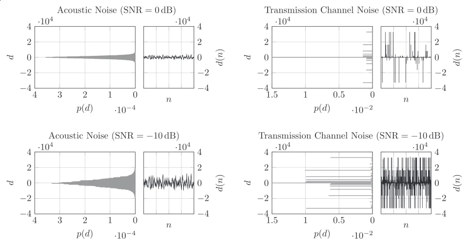
The likelihood in speech enhancement (13) is usually modeled by a common pdf, typically by a Gaussian which is more or less justified by the central limit theorem [3]. In error concealment, however, the noise pdf does not follow any typical distribution and depends on the employed bit mapping. For the further discussion, we define the trans-mission channel noise in error concealment similar to the noise in speech enhancement: The noise d(n) in error concealment will be the difference between the hard-decided speech samples and the transmitted (quantized) one. The histogram of the transmission channel noise turns out to be spiky as can be seen on the right-hand side of Figure 4 for 16 bit uniform PCM quantization, natural-binary bit mapping, and BPSK transmission. The bottom and top spikes in the histograms and the higher ampli-tudes in the waveforms are evoked by bit errors at bit positions close to the most significant bit (MSB).

In the case of acoustic noise, increasing the noise power (decreasing the SNR) naturally results in higher noise sig-nal levels and an increasing width of the time-domain noise histogram (cf. car noise example on the left hand-side of Figure 4). In the case of the transmission chan-nel noise, with increasing noise power (decreasing SNR), more bit errors occur, resulting in higher peaks belong-ing tod = 0 in the histogram on the right-hand side of Figure 4. However, this increase of noise power scales the height of all high spikes in the histogram (referring to sin-gle bit errors) belonging tod = 0 approximately equally (cf. right-hand side of Figure 4). Thus, while in the case of acoustic noise the noise power is typically associated with thewidthof the noise pdf, in error concealment, the noise power can be related to theheightof spikes in the noise histogram belonging to d = 0 (here: for uniform PCM quantization, natural-binary bit mapping, and BPSK modulation).

5.2 The estimator

Figure 4Normalized time domain histograms and waveforms of car noise and transmission channel noise.Left: normalized time domain histograms and waveforms of car noise; right: normalized time domain histograms and waveforms of transmission channel noise applied to 16 bit speech samples with underlying natural-binary bit mapping. The SNR values were calculated by means of a fixed speech signal level of−26 dBov

and respective noise signal levels, both measured according to ITU-T P.56 [37].

distribution for the prior and the likelihood allows for a closed-form solution. Accordingly, a Gaussian assumption for both the prior and the likelihood results in the Kalman filter Eqs. (20), (21), (22), (23) (cf. Section 3).

In error concealment, the clean speech estimator (29) is a sum due to quantization and the respective finite num-ber of transmittable bit combinations. This estimator is computationally complex but manageable in practice due to the one-dimensional pdfs (cf. discrete terms (28), (31)). Thus, the sum (29) can explicitly be computed at run-time [26]. Interestingly, a closed-form solution of the sum cannot be achieved due to the likelihood which cannot be approximated by a common pdf, as outlined in Section 5.1.

5.3 The prior

As can be seen in Section 2, the prior is the pdf of the propagation error (7). In Section 3, it was assumed that the propagation error is Gaussian distributed, therefore, the prior is modeled by a bivariate Gaussian (18) with a complex-valued argument. In [15], the Gaussian assump-tion is justified with the tradeoff between mathematical manageability and pdf model mismatch. It was shown in [16] that the histogram of the propagation error DFT coefficients differ from a Gaussian (cf. left-hand side of Figure 5). Therefore, in [16] the histogram of the prop-agation error was measured and a parametric pdf was trained and then employed as prior. Furthermore, since

the speech estimates strongly depend on the channel, the propagation error also depends on the channel. Accord-ingly, in [38] the SNR dependency of the propagation error histogram was reported and an SNR-dependent estimator was proposed.

Although in [26] the varianceEs+− ˆs+2is assumed to be zero, the non-Gaussianity of the propagation error pdf pe_¯

¯

e=s− ˆs+ was also observed in the context of error concealment. As can be seen on the right-hand side of Figure 5,pe¯in (32), being measured in a training

process, turns out to be rather super-Gaussian. Further-more, in [26] the dependency of pe¯

¯

e=s− ˆs+ on ˆs+ was investigated revealing different shapes and variances dependent on the amplitude ofˆs+, whilesˆ+ = s+ was assumed there.

The propagation error in error concealment is quasi-continuous, while the prior is discrete. Thus, an inte-gration step (32) is needed in order to discretize the propagation error pdf to obtain the prior. Fortunately, this discretization step can be done during a training pro-cess, resulting in a lookup table which nicely reduces the computational complexity [26].

Figure 5Propagation error histograms measured in a speech enhancement system and in an error concealment system.Left: normalized frequency domain histogram of the propagation errorE¯(k)=S(k)−S+(k)measured in a speech enhancement system from Section 3; right: normalized time domain histogram of the propagation errore¯(n)=s(n)− ˆs+(n)measured in an error concealment system from Section 4 assuming thatE{(s+− ˆs+)2}is zero [26].

as reported in [16]. Please note that the propagation error is also dependent on the algorithm for determining the prediction coefficients, therefore, the change of the algo-rithm involves a new propagation error pdf training in both disciplines.

5.4 Outlook

In this section, we briefly sketch further possible research directions for speech enhancement inspired by error con-cealment. Since one of the key success factors in error concealment is that bit reliability information is exploited, the speech enhancement approach from Section 3 could benefit from using bit likelihoods. This means that instead of (13) the DFT coefficient likelihood (12) is calculated by means of bit likelihoods as in error concealment (cf. (27) and (28)).

In the following, we will estimate the real and imagi-nary parts of the complex-valued speech DFT coefficients separately, as in, e. g., [10]. Assuming that the result-ing real-valued real and imaginary parts of STFT-domain quantities are quantized, their natural-binary representa-tion is possible. In the following, we will introduce the processing steps for the real part only, denoted by super-script ‘re’. Of course, the imaginary part can be treated in the same way employing the same processing steps.

In order to be able to employ a bit-level model for the acoustic channel, we assume that the real part of the speech and the noisy speech DFT coefficients are quantized byMbit. Therefore, those quantities can bijec-tively be mapped into the bit combinations Sre(k) = #

S_0,re(k),Sre_1,(k),. . .,Sre_m,(k),. . .,Sre_M−1,(k) $

and Yre(k) = #

Y_0,re(k),Y_1,re(k),. . .,Y_mre_,(k),. . .,Y_Mre_−1,(k)$, respectively. Due to the fact that speech is distorted by acoustic noise while passing through the acoustic channel, the observed bit combinations at the acoustic channel output Yre(k) may differ from those at the channel input Sre(k).

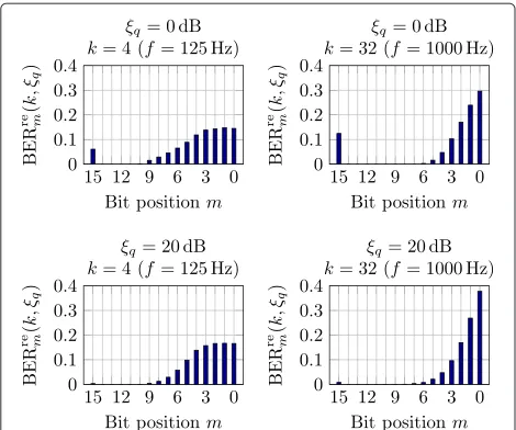
Accordingly, a bit error at bit positionm∈ {0, 1,. . .,M−1} occurs if the received bitY_mre_,(k)is not equal to the trans-mitted one Sre_m,(k). The bit error rate BERre_m(k) can be measured within a training process by comparingSre_m,(k) toY_mre_,(k)for all bit positionsm, individually for each fre-quency bink. Please note that the bit errors also depend on the local SNR in the current time-frequency unit(,k), therefore, the SNR has to be taken into account during the training process. Accordingly, the training steps can be summarized as follows: Using speech and car noise data we generated noisy speech signals at different sig-nal SNR levels. Then, we calculated the short-time spectra of the clean speech, the noise, and the noisy speech sig-nals resulting inS(k),D(k), andY(k)=S(k)+D(k), respectively. Using the resulting DFT coefficients, we cal-culated the true speech powerσ_S2_,(k) = E|S(k)|2and the true noise powerσ_D2_,(k) =E|D(k)|2_{. Using those} two power spectra, we obtained the truea prioriSNR as ξ(k) = σ_S2_,(k)/σ_D2_,(k). Then, we quantized the real part of the clean speech and noisy speech DFT coefficients by 16 bit resulting in the bit combinationsSre(k)andYre(k), respectively. By this means, the whole training data was processed andSre_m,(k)∈Sre(k)andY_mre_,(k)∈Yre(k)were compared to each other. Bit errorsSre_m,(k)=Y_mre_,(k)were counted at bit positionm, frequency bink, and in depen-dence of thea prioriSNR. For the latter, the ideala priori SNRξ(k)was quantized resulting in discretea prioriSNR valuesξq.

The resulting bit error rates BERre_m(k,ξq) were stored in a lookup table; examples can be seen in Figure 6: As expected, at higher SNRs less bits are in error. Typical for car noise, at higher frequencies less bits are in error as compared to lower frequencies.

Figure 6Bit error probabilitiesBERre_m(k,ξq)for differenta priori SNRsξqand frequenciesk.Natural-binary bit representation with

M=16 bit quantization and the MSB (bit positionM−1=15) being the sign bit is used.

lookup tables are then addressed by a quantizeda priori SNR estimateξˆq,(k), computed, e. g., by the well-known decision-directeda prioriSNR estimator [3] and the same quantization intervals as for the training process, result-ing in BERre_m(k,ξˆq,(k)) values. Since each transmitter-sided DFT coefficient S(k) is quantized, it assumes a discrete valueSre,(i) _{withi ∈ 0, 1,. . ., 2}M_−1. Further-more, each Sre,(i) can be mapped to one corresponding bit combinationSre,(i). Then, using the resulting bit error rate BERre_m

k,ξˆq,(k) , the bit likelihood with the given

bitSre,m(i)∈Sre,(i)of theith quantization table entry can be obtained similar to (27) as

P

Y_mre_,(k)S_mre,(i) =

BER_mre_,k,ξˆq,(k) , ifY_mre_,(k)=Sre,m(i),

1−BERre_m,k,ξˆq,(k) , else.

(34)

The bit likelihood describes the probability of an observed bitY_mre_,(k)given a possible channel inputSre,m(i). The coef-ficient likelihood can be obtained using the bit likelihoods similar to (28) as

P %

Yre(k)Sre,(i)

& =

M−1

m=0 P

%

Y_mre_,(k)Sre,_m(i) &

. (35)

By this means, the simple Gaussian assumption for the noise DFT coefficients (13) can be replaced by such a new approach which allows for an environment-specific processing (cf. [39]). This is also illustrated in Figure 7 for ana prioriSNR of 20 dB and the frequency bink= 32 (corresponding to f = 1 kHz): As can be seen, the

Figure 7Coefficient likelihood example.Coefficient likelihoodPYre

(k)Sre,(i)for the specific channel inputSre,(i)=0 calculated by (34) and (35) using trained bit error probabilities

BERre m(k,ξq).

resulting likelihood is a sharp pdf unlike a Gaussian pdf. The Gaussian assumption for noise is typically justified with the central limit theorem assuming that the span of correlation of the noise samples is sufficiently short compared to the frame length [40]. Although this assump-tion is better fulfilled by a wide range of noise types than by speech signals, it can generally be said that it is not fulfilled perfectly in practice by noise signals. Accord-ingly, the likelihood turns out to be a sharper pdf than a Gaussian such as in Figure 7. Please note that the non-Gaussianity of noise DFT coefficients was also reported in [41]. Furthermore, there are publications dealing with speech estimators based on a non-Gaussian assumption for the noise, e. g., [10,12]. Moreover, it was shown in these papers that a more realistic likelihood function (just as the proposed one obtained by training) offers a more precise (acoustic) channel model which can improve estimation results.

The speech prior PSre,(i)S+,re(k) (cf. (17)) can be obtained by integrating (18) according to the PCM quanti-zation intervals(i)(cf. (32)). Here,S+,re(k)is the real part of thea priorispeech estimateS+(k)calculated by, e. g., (16). Using the coefficient likelihood (35) and a speech prior, the recursive MMSE estimation formula turns out to be (cf. (14) and (29))

Sre(k)= 2M_!−1

i=0

Sre,(i)·PYre(k)Sre,(i)·PSre,(i)S+,re(k)

2M_!−1

i=0

PYre(k)Sre,(i)_·PSre,(i)_S+,re (k)

.

(36)

6 Conclusions

This paper provides new insights into links between speech enhancement and error concealment based on recursive MMSE estimation. It turns out that recent approaches to bit error concealment based on a predic-tor are well comparable to iterative approaches in speech enhancement, such as the Kalman filter approach. The main difference between both disciplines are the channel model and the noise pdf. In error concealment, power-ful bit reliability information can be exploited in order to obtain robust estimation results, while in speech enhance-ment the channel is modeled on a sample level without reliable reference. On the other hand, the autoregressive model of speech and the prior computation are well com-parable in both disciplines. Finally, some new research directions are identified for speech enhancement, inspired by error concealment.

Endnotes

a_{Please note that the presented signal model and the}

equations are valid in analogy also in the STFT domain. b_{Please note that for binary phase-shift keying (BPSK)}

modulation, the LLR is obtained byL(xˆm(n))=4·Eb/N0· ym(n)[33].

Appendix

For ease of readability, we will omit the indices and k in this section. In this appendix, we aim at showing that assuming a Gaussian distribution for the propagation error and the acoustic noise, the recursive MMSE estima-tor (14) turns out to be the Kalman filter as in (20), (21), (22), and (23). Employing (17) and (12), (14) turns out to be

As can be seen, the recursive MMSE estimator turns out to be the sum of thea priorispeech estimateS+and a frac-tion with each an integral in the numerator and denom-inatorE = fY−S+. Please note that this fraction is a classical (non-recursive) MMSE estimator, however, with an extra term ‘−S+’ in the pdfpD(·). Assuming a Gaussian distribution forpE¯(·)andpD(·), this classical MMSE esti-mator turns out to be the Wiener filter as we will see later.

Employing (13) forpD(·)and (18) forpE¯(·)as well as

can-celing the constant factors to the exponential functions, the fraction in (38) turns out to be

E=

Integrating with respect to using [42], (40) turns out to be of zeroth and first order, respectively. Integrating with respect to| ¯E|using [42], (41) turns out to be

Thus, substituting (42) forE in (38) and defining ζ = σ2

¯

E/σ 2

Dresults in (cf. (20)-(23))

S=S++ ζ 1+ζ ·

Y−S+. (43)

Competing interests

The authors declare that they have no competing interests.

Acknowledgements

The authors would like to thank Gerald Enzner for inspiring initial discussions toward this paper.

Received: 17 July 2014 Accepted: 7 January 2015

References

1. Trees Van HL,Detection, Estimation and Modulation Theory. Vol 1. Detection, Estimation and Linear Modulation Theory. (Wiley, Hoboken, NJ, USA, 1968) 2. S Kay,Fundamentals of Statistical Signal Processing. Vol 1. Estimation Theory.

(Prentice Hall, Upper Saddle River, NJ, USA, 1993)

4. L Rabiner, R Schafer,Digital Processing of Speech Signals. (Prentice Hall, Upper Saddle River, NJ, USA, 1978)

5. P Vary, R Martin,Digital Speech Transmission: Enhancement, Coding and Error Concealment. (Wiley, Hoboken, NJ, USA, 2006)

6. R Kalman, A new approach to linear filtering and prediction problems. Trans. ASME J. Basic Eng.82, 35–45 (1960)

7. S Haykin,Adaptive Filter Theory. (Prentice Hall, Upper Saddle River, NJ, USA, 2002)

8. R McAulay, M Malpass, Speech enhancement using a soft-decision noise suppression filter. IEEE Trans. Acoustics Speech Signal Process.28(2), 137–145 (1980)

9. Y Ephraim, D Malah, Speech enhancement using a minimum

mean-square error log-spectral amplitude estimator. IEEE Trans. Acoustics Speech Signal Process.33(2), 443–445 (1985)

10. R Martin, inProc. of IEEE International Conference on Acoustics, Speech, and Signal Processing (ICASSP). Speech enhancement using MMSE short time spectral estimation with gamma distributed speech priors, vol. 1 (Orlando, FL, USA, 2002), pp. 253–256

11. I Andrianakis, PR White, inProc. of IEEE International Conference on Acoustics, Speech, and Signal Processing (ICASSP). MMSE speech spectral amplitude estimators with chi and gamma speech priors, vol. 3 (Toulouse, France, 2006), pp. 1068–1071

12. JS Erkelens, RC Hendriks, R Heusdens, J Jensen, Minimum mean-square error estimation of discrete fourier coefficients with generalized gamma priors. IEEE Trans Audio Speech Lang. Process.15(6), 1741–1752 (2007)

13. P Scalart, JV Filho, inProc. of IEEE International Conference on Acoustics, Speech, and Signal Processing (ICASSP). Speech enhancement based on a priori signal to noise estimation, vol. 2 (Atlanta, GA, USA, 1996), pp. 629–632

14. KK Paliwal, A Basu, inProc. of IEEE International Conference on Acoustics, Speech, and Signal Processing (ICASSP). A speech enhancement method based on Kalman filtering (Dallas, TX, USA, 1987), pp. 177–180 15. E Zavarehei, S Vaseghi, inProc. of ISCA INTERSPEECH 2005. Speech

enhancement in temporal DFT trajectories using Kalman filters (Lisbon, Portugal, 2005), pp. 2077–2080

16. T Esch, P Vary, inProc. of IEEE International Conference on Acoustics, Speech, and Signal Processing (ICASSP). Speech enhancement using a modified Kalman filter based on complex linear prediction and supergaussian priors (Las Vegas, NV, USA, 2008), pp. 4877–4880

17. T Esch, P Vary, inProc. of International Workshop on Acoustic Echo and Noise Control (IWAENC). Modified Kalman filter exploiting interframe correlation of speech and noise magnitudes (Seattle, WA, USA, 2008), pp. 1–4 18. N Görtz, inProc. of IEEE International Symposium on Information Theory.

Joint source channel decoding using bit-reliability information and source statistics (Cambridge, MA, USA, 1998), p. 9

19. T Fingscheidt, P Vary, Softbit speech decoding: a new approach to error concealment. IEEE Trans. Speech Audio Process.9(3), 240–251 (2001) 20. F Lahouti, AK Khandani, Soft reconstruction of speech in the presence of

noise and packet loss. IEEE Trans. Audio Speech Lang. Process.15(1), 44–56 (2007)

21. AM Pourmir, F Lahouti, inProc. of 16th International Conference on Software, Telecommunications, and Computer Networks (SoftCOM). Joint source channel speech decoding using long-term residual redundancy (Split, Croatia, 2008), pp. 329–333

22. AJ Jameel, H Adnan, Y Xiaohu, A Hussain, inProc. of Developments in eSystems Engineering (DeSE). Error concealment of EVRC speech decoder using residual redundancy (Abu Dhabi, United Arab Emirates, 2009), pp. 84–88

23. S Han, F Pflug, T Fingscheidt, inProc. of 21th European Signal Processing Conference (EUSIPCO). Improved AMR wideband error concealment for mobile communications (Marrakech, Morocco, 2013), pp. 1–5 24. M Adrat, J Spittka, S Heinen, P Vary, inProc. of IEEE Workshop on Speech

Coding (SCW). Error concealment by near optimum MMSE-estimation of source codec parameters (Delavan, WI, USA, 2000), pp. 84–86 25. F Pflug, T Fingscheidt, inProc. of 134th International Audio Engineering

Society (AES) Convention. Delayless robust DPCM audio transmission for digital wireless microphones (Rome, Italy, 2013), pp. 1–8

26. F Pflug, T Fingscheidt, Robust ultra-low latency soft-decision decoding of linear PCM audio. IEEE Trans. Audio Speech Lang. Process.21(11), 2324–2336 (2013)

27. A Papoulis, U Pillai,Probability, Random Variables and Stochastic Processes, 4th edn. (McGraw-Hill, New York, NY, USA, 2002)

28. T Esch, Model-based speech enhancement exploiting temporal and spectral dependencies. PhD thesis, Rheinisch-Westfälische Technische Hochschule Aachen, Aachen, Germany (2012). http://darwin.bth.rwth-aachen.de/opus3/volltexte/2012/4035/pdf/4035.pdf

29. R Martin, PU Heute, Eds Antweiler C,Advances in Digital Speech Transmission. (Wiley, Hoboken, NJ, USA, 2008)

30. R Martin, Noise power spectral density estimation based on optimal smoothing and minimum statistics. IEEE Trans. Speech Audio Process. 9(5), 504–512 (2001)

31. I Cohen, Noise spectrum estimation in adverse environments: Improved minima controlled recursive averaging. IEEE Trans. Speech Audio Process. 11(5), 466–475 (2003)

32. T Gerkmann, RC Hendriks, Unbiased MMSE-based noise power estimation with low complexity and low tracking delay. IEEE Trans. Audio Speech Lang. Process.20(4), 1383–1393 (2012)

33. J Hagenauer, Source-controlled channel decoding. IEEE Trans. Commun. 43(9), 2449–2457 (1995)

34. T Fingscheidt, P Vary, inProc. IEEE International Conference on Acoustics, Speech, and Signal Processing (ICASSP). Robust speech decoding: A universal approach to bit error concealment, vol. 3 (Munich, Germany, 1997), pp. 1667–1670

35. GDT Schuller, B Yu, D Huang, B Edler, Perceptual audio coding using adaptive pre- and post-filters and lossless compression. IEEE Trans. Speech Audio Process.10(6), 379–390 (2002)

36. I Cohen, B Berdugo, Noise estimation by minima controlled recursive averaging for robust speech enhancement. IEEE Signal Process. Lett.9(1), 12–15 (2002)

37. Telecommunication Standardization Sector of the International Telecommunication Union (ITU-T). Recommendation ITU-T P.56, Objective Measurement of Active Speech Level (1993). http://www.itu. int/rec/T-REC-P/

38. T Esch, P Vary, inProc. of IEEE International Conference on Acoustics, Speech, and Signal Processing (ICASSP). Model-based speech enhancement using SNR dependent MMSE estimation (Prague, Czech Republic, 2011), pp. 4073–4076

39. T Fingscheidt, S Suhadi, S Stan, Environment-optimized speech enhancement. IEEE Trans. Audio Speech Lang. Process.16(4), 825–834 (2008)

40. T Lotter, P Vary, Speech enhancement by MAP spectral amplitude estimation using a super-gaussian speech model. EURASIP J. Appl. Signal Process.7, 1110–1126 (2005)

41. B Fodor, T Fingscheidt, inProc. of European Signal Processing Conference (EUSIPCO). MMSE Speech Spectral Amplitude Estimation Assuming Non-Gaussian Noise (Barcelona, Spain, 2011), pp. 2314–2318 42. IS Gradshteyn, IM Ryzhik,Table of Integral, Series, and Products, 4th edn.

(Academic Press, New York, NY, USA, 1965)

Submit your manuscript to a

journal and benefi t from:

7 Convenient online submission 7 Rigorous peer review

7 Immediate publication on acceptance 7 Open access: articles freely available online 7 High visibility within the fi eld

7 Retaining the copyright to your article