New DEA/Location Models with Interval Data

829

Int. J. Data Envelopment Analysis (ISSN 2345-458X)

Vol.3, No.4, Year 2015 Article ID IJDEA-00342, 12 pages

Research Article

New DEA/Location Models with Interval Data

Naser Ghasemi

, Esmaeel Najafi

, Hosein Shams

(a) Department of Industrial Engineering, Science and Research Branch, Islamic Azad University,

Tehran, Iran

(b) Department of Industrial Engineering, Science and Research Branch, Islamic Azad University,

Tehran, Iran

(c) Department of Industrial and Mechanical Engineering, Islamic Azad University, Qazvin, Iran

Received 11 February 2016, Revised 20 May 2016, Accepted 28 May 2016

Abstract

Recently the concept of facility efficiency, which defined by data envelopment analysis (DEA), introduced as a location modeling objective, that provides facilities location’s effect on their performance in serving demands. By combining the DEA models with the location problem, two types of “efficiencies” are optimized: spatial efficiency which measured by finding the least cost location and allocation patterns for facilities, and the facility efficiency in serving demands which measured by DEA efficiency score. In this paper, location-allocation models with DEA in interval inputs and outputs environments are combined. A new pair of interval DEA/location models are constructed and run.

Keywords:

*

Corresponding Author: [email protected]

830

Many types of location-allocation models have been presented to find optimal facilities location patterns with respect to several criteria like cost, demands coverage, time and others. Some of these models have been formulated in a multi objective programming framework eliciting trade-offs among these sometimes conflicting objectives (Klimberg and Ratick 2008). Most of these models follow just spatial efficiency and disregard to facilities efficiency, while final purpose of facilities installation and location is maximization of yield and efficiency and to achieve this purpose, the facilities efficiency in serving demands must be maximized. On the other hand, minimization of cost and time and maximization of demands coverage aren’t enough to achieve optimal efficiency. Therefore, some models recently developed that use the concept of efficiency as defined by DEA as another location modeling objective to help providing insights into the performance of facilities at different potential sites. However, the previous models do not deal with imprecise data and assume that all input and output data are exactly known. In real world condition, however, this assumption may not always be true. Due to the existence of uncertainty, DEA sometimes faces the situation of imprecise data, especially when a set of decision-making units (DMUs) contains missing data, judgment data, forecasting data or ordinal preference information. Generally speaking, uncertain information or imprecise data can be expressed in interval or fuzzy

management or operation efficiency of a set of DMUs in interval and/or fuzzy environments is a worth-studying problem. This is the need of both the developments of DEA theory and methodology and its real applications (Wang et al. 2005). Therefore, in this paper, location-allocation models are combined with DEA in interval inputs and outputs environments to improve performance of these models.

Location-allocation problems have several types. We have used uncapacitated facility location problem (UPLP) model and the capacitated facility location problem (CPLP) model as the base location modeling framework for our model formulations. The uncapacitated facility location problems take a great variety of forms, depending on the nature of the objective function (mini sum, mini max, problems with covering constraints). The uncapacitated model assumes each facility has unlimited capacity, and as a result, if a facility supplies a demand node, it will satisfy all the demand, i.e., only one facility is necessary to serve a particular demand. The mathematical formulation of the UPLP is

𝑚𝑖𝑛 𝑐𝑘𝑙 𝑙

𝑑𝑒𝑚𝑙𝑡𝑘𝑙+ 𝐹𝑘𝑡𝑘 𝑘 𝑘

(1)

s.t:

𝑡𝑘𝑙 = 1 𝑘

∀𝑙

𝑡𝑘𝑙 ≤ 𝑡𝑘 ∀𝑘, 𝑙 𝑡𝑘𝑙, 𝑡𝑘 = 0,1

Where

831 𝑐_𝑘𝑙: cost of shipping one unit of demand from facility k to demand l,

𝐹𝑘: fixed cost of opening/using facility k, 𝑑𝑒𝑚𝑙: the amount of demand at node,

𝑡𝑘 =

1 𝑖𝑓 𝑓𝑎𝑐𝑖𝑙𝑖𝑡𝑦 𝑘 𝑜𝑝𝑒𝑛𝑑

0 𝑂𝑊

𝑡𝑘𝑙=

1 𝑖𝑓 𝑓𝑎𝑐𝑖𝑙𝑖𝑡𝑦 𝑘 𝑠𝑒𝑟𝑣𝑒𝑠 𝑑𝑒𝑚𝑎𝑛𝑑 𝑙

0 𝑂𝑊

In the CPLP, a number of capacitated facilities are to be located among possible sites in order to satisfy demands of customers by minimizing total costs of transportation and fixed charges of establishing facilities. The CPLP has been effectively implemented to solve real-world applications such as plants location, power stations location, warehouses location, to just name a few. The CPLP is generalization of the simple plant location problem. In the CPLP each facility has limited capacity and so more than one facility may supply a demand node. The formulation for the CPLP is:

𝑚𝑖𝑛 𝑐𝑘𝑙 𝑙

𝑏𝑘𝑙 + 𝐹𝑘𝑡𝑘 𝑘 𝑘

(2)

s.t:

𝑡𝑘𝑙 ≥ 1 𝑘

∀𝑙

𝑡𝑘𝑙 ≤ 𝑡𝑘 ∀𝑘, 𝑙

𝑏𝑘𝑙 = 𝑑𝑒𝑚𝑙 ∀𝑙 𝑘

𝑏𝑘𝑙 ≤ 𝑀𝑖𝑛 𝑑𝑒𝑚𝑙, 𝑐𝑎𝑝𝑘 𝑡𝑘 ∀𝑘, 𝑙 𝑡𝑘𝑙, 𝑡𝑘= 0,1

𝑏𝑘𝑙 ≥ 0

Where

𝑐𝑎𝑝𝑘: capacity of facility k

𝑏_𝑘𝑙: amount of units which shipped from facility k to demand location l. The other parameters and variables are the same with model (1).

In this paper, we combine UPLP and CPLP with DEA in interval inputs and outputs to find optimal and efficient facility location/allocation patterns.

2. Literature Review

Location analysis is a specialized branch of combinatorial optimization that has grown from early foundations to maturity, with most growth occurring since the 1960s. A wide range of problems has emerged, which may be characterized in general as finding optimal locations for facilities.

832

location problem that was based on a linear programming dual formation. A simple ascent and adjustment procedure frequently produces optimal dual solutions, which in turn often correspond directly to optimal integer primal solutions. If not, a branch-and-bound procedure completes the solution process. Erlenkotter (1978)’s method used Lagrangian relaxation with solutions to the dual problem achieves significantly quicker results in finding integer solutions, and can itself be said to be a milestone in algorithmic terms. Guignard and Spielberg (1979) give a direct dual method, consisting of several phases (each of which appears essential for some data), to resolve a strong relaxed form of the mixed plant location problem (mixed in the sense of allowing capacitated as well as uncapacitated plants) with additional constraints over the integer variables (user specified, or derived from the data themselves). Bilde and krarup (1977) presented a sharp lower bounds and efficient algorithms for the simple plant location problem. Cornuejols et al. (1991) presented an excellent theoretical analysis of all possible Lagrangian relaxations and the linear programming relaxation for the CPLP.

DEA is an extension of Farrell (1957)'s idea of linking the computation of technical efficiency with production frontiers. The first DEA model was developed by Charnes et al. (1978). The CCR model is a fractional programming model, which measures the relative technical

efficiency of a firm by calculating the ratio of weighted sum of its outputs to the weighted sum of its inputs. The fractional program is run for each firm to determine the set of input-output weights, which maximizes the efficiency of that firm subject to the condition that no firm can have a relative efficiency score greater than unity for that set of weights. Thus, the DEA model calculates a unique set of factor weights for each firm. The set of weights has the following characteristics: It maximizes the efficiency of the firm for which it is calculated and it is feasible for all firms. The model (3) is linear programming of CCR model

Max uryrk r

uryrj− vixij s

r=1 r

𝑗 = 1,2, … , 𝑛 3

viyik i

= 1

ur, 𝑣𝑖≥0 r = i, … , m , r = 1, … , s

Here uij, 𝑣𝑟𝑗 are inputs and outputs of 𝐷𝑀𝑈𝑗 and

ur, 𝑣𝑖≥0 are the variable weights to be

833

Klimberg and Ratick (2008) mentioned that Fisher and Rushton (1979), Desai and Storbeck (1990), Desai et al. (1995), and Athanassopoulos and Storbeck (1995), are a series of related papers which applied DEA to measure the relative spatial efficiency of location decisions. As part of their DEA models, they used two measures of access as input variables, the total travel distance and the extent of non-coverage populations not within a specified distance of a facility (Klimberg and Ratick 2008). Thomas et al. (2002) have broadened the classic anti-center models to include generalized-distance measures. It includes in the inherent proximity measures other cost/benefit metrics. Unlike the classic data envelopment analysis (DEA), the combined location/DEA model proposed in their research assumes disposability of input/output's only. It represents a more flexible formulation. The locations of multiple sites are analyzed using a binary integer program, while evaluation is performed by the full strength of a DEA model. Through a case study, they show how location and DEA models can be used together to more realistically characterize a sitting decision. In previews studies, these two objectives i.e., spatial efficiency and facility efficiency have not been simultaneously applied to find and evaluate solutions to location problems. However, Klimberg and Ratick (2008) combined the DEA problem with the location problem and spatial efficiency with the facility

efficiency were simultaneously optimized. Their model does not deal with imprecise data and assumes that all inputs and outputs data are exactly known. In real world situations, however, this assumption may not always be true. Due to the existence of uncertainty, we sometimes face the situation of imprecise data, especially when a set of decision-making units (DMUs) contains missing data, judgment data, forecasting data or ordinal preference information. Generally speaking, uncertain information or imprecise data can be expressed in interval or fuzzy numbers. Therefore, how to evaluate the management or operation efficiency of a set of DMUs in interval and/or fuzzy environments is a worth-studying problem. This is the need of both the

developments of DEA theory and

methodology and its real applications (Wang et al. (2005) ). So in the next section we develop and present formulations combining the uncapacitated and capacitated facility location problem with the DEA problem in interval inputs and outputs environments.

3. Model Development

834

(Wang et al. (2005)). However, in real world condition many complicated factors are involved that makes difficult to measure inputs and outputs precisely. This makes a case where we need to measure the efficiency of DMUs with inexact values or interval data.

3.1. CCR Model With Interval Data

The approach proposed in this paper is based on Kabnurkar (2001)’s research. He presupposed that the decision-maker can define the risk free and impossible bounds for each interval input and output. Risk-free bounds are the conservative values that are most realistically attainable in real world condition, whereas impossible bounds are associated with those values, which represent management scenarios that are the least realistic. The risk-free and impossible bounds are used for determining the membership functions for the input and output data. All membership functions are assumed to vary linearly between the bounds. In addition, all membership functions have a value equal to zero at the impossible bounds and a value equal to one at the risk-free bounds (Kabnurkar 2001).

If superscripts 0 and 1 represent impossible and risk-free bounds for input data, then the membership function associated with the 𝑖𝑡ℎ fuzzy input (𝑥𝑖𝑗) for the 𝑗𝑡ℎ DMU is given by:

𝜇𝑥 𝑥𝑖𝑗 =

𝑥𝑖𝑗𝑜 − 𝑥𝑖𝑗 𝑥𝑖𝑗𝑜 − 𝑥𝑖𝑗1

4

Furthermore, if superscripts 0 and 1 represent impossible and risk-free bounds for output

data, then the membership function associated with the 𝑟𝑡ℎ output (𝑦𝑟𝑗) for the 𝑗𝑡ℎ DMU is given by:

𝜇𝑦 𝑦𝑟𝑗 =

𝑦𝑟𝑗 − 𝑦𝑟𝑗1 𝑦𝑟𝑗0 − 𝑦𝑟𝑗1

5

Both (𝑥_𝑖𝑗) and(𝑦_𝑟𝑗)can be expressed in terms of the risk-free and impossible bounds and the membership functions as follows:

𝑥𝑖𝑗 = 𝑥𝑖𝑗𝑜 − 𝑥𝑖𝑗𝑜 − 𝑥𝑖𝑗1 𝜇𝑥 6

𝑦𝑟𝑗 = 𝑦𝑟𝑗0 − 𝑦𝑟𝑗1 𝜇𝑦 + 𝑦𝑟𝑗1 (7)

Using these definitions, the model (3) can be modified as follows: Find u and v such that,

𝑀𝑎𝑥 𝑢𝑟

𝑟

[ 𝑦𝑟𝑘0 − 𝑦𝑟𝑘1 𝜇𝑦 + 𝑦𝑟𝑘1 ]

s.t: (8)

𝑣𝑖

𝑖

[𝑥𝑖𝑘𝑜 − 𝑥𝑖𝑘𝑜 − 𝑥𝑖𝑘1 𝜇𝑥] = 1

𝑢𝑟

𝑟

[ 𝑦𝑟𝑗0 − 𝑦𝑟𝑗1 𝜇𝑦 + 𝑦𝑟𝑗1] − 𝑣𝑖 𝑖

[𝑥𝑖𝑗𝑜 − 𝑥𝑖𝑗𝑜− 𝑥𝑖𝑗1 𝜇𝑥] ≤ 0

𝑣𝑖≥ 𝜀 , 𝑢𝑟≥ 𝜀, 𝑖 = 1, … , 𝑚, 𝑟 = 1, … , 𝑠

As was mentioned in Carlsson and Korhonen (1986), the decision for the above model is achieved when,

𝜇𝑥 = 𝜇𝑦 = 𝜇 = 𝑚𝑖𝑛 𝜇𝑥, 𝜇𝑦 (9)

So, the model (8) can be written as

𝑀𝑎𝑥 𝑢𝑟

𝑟

[ 𝑦𝑟𝑘0 − 𝑦𝑟𝑘1 𝜇 + 𝑦𝑟𝑘1 ]

s.t: (10)

𝑣𝑖

𝑖

[𝑥𝑖𝑘𝑜 − 𝑥𝑖𝑘𝑜 − 𝑥𝑖𝑘1 𝜇 ] = 1

𝑢𝑟

𝑟

[ 𝑦_𝑟𝑗0 _{− 𝑦} 𝑟𝑗

1 _{𝜇 + 𝑦}

𝑟𝑗

1_{] − 𝑣}

𝑖 𝑖

[𝑥_𝑖𝑗𝑜 _{− 𝑥}

𝑖𝑗𝑜− 𝑥𝑖𝑗1 𝜇 ] ≤ 0

𝑣𝑖≥ 𝜀 , 𝑢𝑟≥ 𝜀, 𝑖 = 1, … , 𝑚, 𝑟 = 1, … , 𝑠

835

intervals to observe the variations of the efficiency profile. Here, μ = 0 would yield overly optimistic values of technical efficiency and μ = 1 would yield ultra conservative values.

3.2. Combined UPLP/interval DEA model

In this section, we combine UPLP model and CCR model with DEA model by interval data i.e., model (10), which have been presented in previews section. The model (10) is non-linear because of existing 𝜇𝑣𝑖and 𝜇𝑢𝑟, therefore, to make it easier to solve, we convert it into a linear programming model as follows:

𝜇𝑢𝑟 = 𝑞𝑟 => 0 ≤ 𝑞𝑟 < 𝑢𝑟 (11) 𝜇𝑣𝑖= 𝑝𝑖 => 0 ≤ 𝑝𝑖 < 𝑣𝑖 12

With replacement of 𝑝𝑖and 𝑞𝑟in model (10) we get model (13).

𝑀𝑎𝑥 𝑞𝑟

𝑟

[ 𝑦𝑟𝑘0 − 𝑦𝑟𝑘1 + 𝑢𝑟 𝑦𝑟𝑘1 ]

s.t: (13)

𝑖

[𝑣𝑖𝑥𝑖𝑘𝑜 − 𝑝𝑖 𝑥𝑖𝑘𝑜 − 𝑥𝑖𝑘1 ] = 1

𝑞𝑟 𝑟

[ 𝑦𝑟𝑗0 − 𝑦𝑟𝑗1 +𝑢𝑟𝑦𝑟𝑗1] − [𝑣𝑖𝑥𝑖𝑗𝑜−𝑝𝑖 𝑥𝑖𝑗𝑜 − 𝑥𝑖𝑗1 ] 𝑖

≤ 0

𝑣𝑖≥ 𝜀 , 𝑢𝑟≥ 𝜀, 0 ≤ 𝑞𝑟< 𝑢𝑟, 0 ≤ 𝑝𝑖< 𝑣𝑖 ,

𝑖 = 1, … , 𝑚, 𝑟 = 1, … , 𝑠

The model (14) maximizes the sum of the efficiencies for all DMUs. Where 𝑑𝑘is the level of inefficiency of DMU k. (Klimberg and Ratick 2008)

𝑀𝑎𝑥 (1 − 𝑑𝑘)

𝑘

s.t: (14)

𝑣𝑖

𝑖

𝑥𝑖𝑘 = 1 ∀𝑘

𝑢𝑟

𝑟

𝑦𝑟𝑘+𝑑𝑘 = 1 ∀𝑘

𝑢𝑟

𝑟

𝑦𝑟𝑗 − 𝑣𝑖 𝑖

𝑥𝑖𝑗 ≤ 0 ∀𝑗, 𝑘

𝑑𝑘, 𝑣𝑖, 𝑢𝑟≥ 0 ∀𝑖, 𝑗, 𝑘, 𝑖 = 1, … , 𝑚, 𝑟 = 1, … , 𝑠

By Combination the model (13) and the model (14), we will get the model (15).

𝑀𝑎𝑥 (1 − 𝑑𝑘)

𝑘

s.t: (15)

𝑖

[𝑣𝑖𝑥𝑖𝑘𝑜 − 𝑝𝑖 𝑥𝑖𝑘𝑜 − 𝑥𝑖𝑘1 ] = 1

𝑟

[𝑞𝑟 𝑦𝑟𝑘0 − 𝑦𝑟𝑘1 + 𝑢𝑟 𝑦𝑟𝑘1 ] + 𝑑𝑘= 1

𝑞𝑟 𝑟

𝑦𝑟𝑗0 − 𝑦𝑟𝑗1 + 𝑢𝑟 𝑦𝑟𝑗1 − [𝑣𝑖𝑥𝑖𝑗𝑜− 𝑝𝑖 𝑥𝑖𝑗𝑜 − 𝑥𝑖𝑗1 ] 𝑖

≤ 0

𝑣𝑖≥ 𝜀 , 𝑢𝑟≥ 𝜀, 0 ≤ 𝑞𝑟< 𝑢𝑟, 0 ≤ 𝑝𝑖< 𝑣𝑖 ,

𝑖 = 1, … , 𝑚, 𝑟 = 1, … , 𝑠

The combination of model (15) with model UPLP (model (1)) results in the final model, i.e, model (16).

𝑀𝑎𝑥 1 − 𝑑𝑘𝑙

𝑙 𝑘

𝑀𝑖𝑛 𝑐𝑘𝑙

𝑙

𝑑𝑒𝑚𝑙𝑡𝑘𝑙+ 𝐹𝑘𝑡𝑘 𝑘 𝑘

(16)

s.t:

𝑡𝑘𝑙 = 1

𝑘

∀𝑙

𝑡𝑘𝑙≤ 𝑡𝑘 ∀𝑘, 𝑙

[𝑣𝑖𝑘𝑙𝑥𝑖𝑘𝑙𝑜 − 𝑝𝑖𝑘𝑙 𝑥𝑖𝑘𝑙𝑜 − 𝑥𝑖𝑘𝑙1 ] = 𝑡𝑘𝑙 i

∀𝑖, 𝑘, 𝑙

[𝑞𝑟𝑘𝑙 𝑦𝑟𝑘𝑙0 − 𝑦𝑟𝑘𝑙1 + 𝑢𝑟𝑘𝑙 𝑦𝑟𝑘𝑙1 ] 𝑟

+ 𝑑𝑘𝑙= 𝑡𝑘𝑙 ∀𝑟, 𝑘, 𝑙

𝑞𝑟𝑠ℎ 𝑦𝑟𝑠ℎ0 − 𝑦𝑟𝑠ℎ1 + 𝑢𝑟𝑘𝑙 𝑦𝑟𝑠ℎ1 𝑟

− 𝑣𝑖𝑘𝑙𝑥𝑖𝑠ℎ𝑜 − 𝑝𝑖𝑠ℎ 𝑥𝑖𝑠ℎ𝑜 − 𝑥𝑖𝑠ℎ1 ≤ 0 𝑙

836

𝜀𝑡𝑘𝑙≤ 𝑞𝑟𝑘𝑙 ≤ 𝑢𝑟𝑘𝑙

𝜀𝑡𝑘𝑙≤ 𝑝𝑖𝑘𝑙≤ 𝑣𝑖𝑘𝑙,

𝑖 = 1, … , 𝑚, 𝑟 = 1, … , 𝑠

Where

𝑥𝑖𝑘𝑙𝑜 : impossible bound for ith input of DMU kl 𝑥𝑖𝑘𝑙1 : risk free bound for ith input of DMU kl 𝑦𝑟𝑘𝑙0 : risk free bound for rth output of DMU kl 𝑦𝑟𝑘𝑙1 : impossible bound for rthoutput of DMU kl 𝐹𝑘: fixed cost of opening/using facilityk 𝑑𝑒𝑚𝑙: the amount of demand at node l

𝑡𝑘 =

1 𝑖𝑓 𝑓𝑎𝑐𝑖𝑙𝑖𝑡𝑦 𝑘 𝑜𝑝𝑒𝑛𝑑

0 𝑂𝑊

𝑡𝑘𝑙=

1 𝑖𝑓 𝑓𝑎𝑐𝑖𝑙𝑖𝑡𝑦 𝑘 𝑠𝑒𝑟𝑣𝑒𝑠 𝑑𝑒𝑚𝑎𝑛𝑑 𝑙

0 𝑂𝑊

𝑐𝑘𝑙: cost of shipping one unit of demand from facility k to demand l,

𝑑𝑘𝑙: the level of inefficiency of DMU kl. 𝑣𝑖𝑘𝑙:input weight for 𝑖𝑡ℎ input of DMU kl 𝑢𝑟𝑘𝑙: output weightfor 𝑟𝑡ℎ output of DMU kl

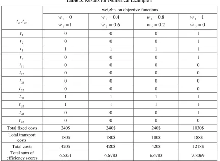
3.3. Numerical Example I

An example with four facilities and two demand nodes was created to test model (16). The input and output values, fixed cost of opening/using facilities, the amount of demand at node l and cost of shipping one unit of demand from facilities to demand nodes are listed in Table 1 and Table 2. The model (16) was run with the data discussed above by assigning weights to objective functions and yielded the following results which are shown in Table 3 and Table 4. Here, w1 is the weight

on the DEA objective function and w2 is the

weight on the cost objective function.

3.4.Combined CPLP/interval DEA model

Like the section 3.2, we combine the CPLP model (model (2)) with the model (15) and get the simultaneous CPLP/interval DEA model i.e, model (17).

𝑀𝑎𝑥 1 − 𝑑𝑘𝑙

𝑙 𝑘

𝑀𝑖𝑛 𝑐𝑘𝑙

𝑙

𝑏𝑘𝑙+ 𝐹𝑘𝑡𝑘 𝑘 𝑘

(17)

𝑡𝑘𝑙 ≥ 1

𝑘

∀𝑙

𝑡𝑘𝑙≤ 𝑡𝑘 ∀𝑘, 𝑙

𝑏𝑘𝑙

𝑖

=𝑑𝑒𝑚𝑙 ∀𝑘

𝑏𝑘𝑙≤ [𝑑𝑒𝑚𝑙,𝑦𝑘𝑙0]𝑡𝑘 ∀𝑘, 𝑙

[𝑣𝑖𝑘𝑙𝑥𝑖𝑘𝑙𝑜 − 𝑝𝑖𝑘𝑙 𝑥𝑖𝑘𝑙𝑜 − 𝑥𝑖𝑘𝑙1 ] = 𝑡𝑘𝑙 i

∀𝑖, 𝑘, 𝑙

[𝑞𝑟𝑘𝑙 𝑦𝑟𝑘𝑙0 − 𝑦𝑟𝑘𝑙1 + 𝑢𝑟𝑘𝑙 𝑦𝑟𝑘𝑙1 ] 𝑟

+ 𝑑𝑘𝑙= 𝑡𝑘𝑙 ∀𝑟, 𝑘, 𝑙

𝑞𝑟𝑠ℎ 𝑦𝑟𝑠ℎ0 − 𝑦𝑟𝑠ℎ1 + 𝑢𝑟𝑘𝑙 𝑦𝑟𝑠ℎ1 𝑟

− 𝑣𝑖𝑘𝑙𝑥𝑖𝑠ℎ𝑜 − 𝑝𝑖𝑠ℎ 𝑥𝑖𝑠ℎ𝑜 − 𝑥𝑖𝑠ℎ1 ≤ 0 𝑙

𝑡𝑘𝑙, 𝑡𝑘= 0,1

𝜀𝑡𝑘𝑙≤ 𝑞𝑟𝑘𝑙 ≤ 𝑢𝑟𝑘𝑙

𝜀𝑡𝑘𝑙≤ 𝑝𝑖𝑘𝑙≤ 𝑣𝑖𝑘𝑙,

𝑏𝑘𝑙≥𝑡𝑘𝑙

Here, 𝑏𝑘𝑙is amount of shipping units from facility k to demand node l. The other parameters and variable are the same with the model (16).

3.5. Numerical Example II

837

Table 1. Fixed cost of opening facilities,input/output values and cost of shipping one unit of demand from facilities to demand nodes

𝑐𝑘𝑙

output values input values

demand node fixed cost of

opening facilities facilities 5$ [31,38] [11,17] 1 220$ 1 9$ [32,37] [12,15] 2 1 6$ [26,30] [11,15] 1 270$ 2 7$ [27,31] [12,16] 2 2 5$ [25,30] [5,13] 1 240$ 3 7$ [27,31] [11,17] 2 3 9$ [24,32] [6,12] 1 300$ 4 7$ [31,38] [11,18] 2 4

Table 2. Demand requirement of each demand node

2 1 demand node 20 8 amount of demand

Table 3. Results for Numerical Example I weights on objective functions

1 2 1 0 w w   1 2 0.8 0.2 w w   1 2 0.4 0.6 w w   1 2 0 1 w w   , k kl t t 1 0 0 0 1 t 1 0 0 0 2 t 1 1 1 1 3 t 1 0 0 0 4 t 0 0 0 0 11 t 0 0 0 0 12 t 0 0 0 0 21 t 0 0 0 0 22 t 1 1 1 1 31 t 1 1 1 1 32 t 1 0 0 0 41 t 0 0 0 0 42 t 1030$ 240$ 240$ 240$

Total fixed costs

188$ 180$ 180$ 180$ Total transport costs 1218$ 420$ 420$ 420$ Total costs 7.8069 6.6783 6.6783 6.5351

838

Table 4. Efficiency scores for DMUs in Numerical Example I

1 2 1 0 w w   1 2 0.8 0.2 w w   1 2 0.4 0.6 w w   1 2 0 1 w w   weights on objective functions DMUs 1 1 1 1 (1,1) 1 1 1 1 (1,2) 1 1 1 1 (2,1) 1 1 1 1 (2,2) 1 0.3404 0.3404 0.025 (3,1) 0.8069 0.3379 0.3379 0.5101 (3,2) 1 1 1 1 (4,1) 1 1 1 1 (4,2)

Table 5. Results of Numerical Example II weights on objective functions

1 2 1 0 w w   1 2 0.8 0.2 w w   1 2 0.4 0.6 w w   1 2 0 1 w w   , k kl t t 1 1 1 1 1 t 1 1 1 1 2 t 1 1 1 1 3 t 1 0 0 0 4 t 1 1 1 1 11 t 0 0 0 0 12 t 0 0 0 0 21 t 0 0 0 1 22 t 1 0 0 1 31 t 0 1 1 1 32 t 1 0 0 0 41 t 1 0 0 0 42 t 1030$ 730$ 730$ 730$

Total fixed costs

195$ 188$

188$ 188$

Total transport costs

1225$ 608$ 608$ 608$ Total costs 8 7.5082 7.5082 5.9643

Total sum of efficiency scores

Table 6. Efficiency scores for DMUs in Numerical Example II

839 4. Conclusion

In this paper, we combined location/allocation models with DEA in interval inputs and outputs environments to improve performance of these models. Solving for the DEA efficiency measure, simultaneously with other location modeling objectives, provides a promising rich approach to multi objective location problems. The ability to use location models to test trade-offs between spatial efficiency and facility efficiency provides a promising new rich approach for multi objective location analysis. We presented a new pair of location/DEA models for dealing with interval data. The presented models used the interval CCR model and combined it with UPLP and CPLP models to optimize two efficiencies, spatial efficiency and facilities efficiency. Due to the existence of uncertainty in real world conditions, our models dealt with interval inputs and outputs. The models were run with the data discussed in Numerical Example I and the results obtained. Since interval efficiencies measure the performances of DMUs more comprehensively than the traditional DEA efficiency, they are expected to have widely potential applications in the future.

References

[1] Athanassopoulos AD, Storbeck JE (1995) Non-parametric models for spatial efficiency. The Journal of Productivity Analysis 6:225–45 [2] Blide O, Krarup J (1977) Sharp Lower

Bound and Efficient Algorithms for the simple Plant Location Problem. Annals of Discrete Mathematics 1:79-97

[3] Carlsson, C, Korhonen P (1986) A parametric approach to fuzzy linear programming. Fuzzy Sets and Systems 20:17-30

[4] Charnes A, Cooper WW, Rhodes E (1978) Measuring the efficiency of decision making units. European Journal of Operational Research 2:429–444

[5] Cornuejols G, Sridharan R, Thizy JM (1991) A comparison of heuristics and relaxations for the capacitated plant location problem. European Journal of Operational Research 50:280–297

[6] Desai A, Haynes K, Storbeck JE (1995) A spatial efficiency for the support of location decision. In: Charnes A, Cooper WW, Lewin A, Seiford L, editors. Data envelopment

analysis: theory, methodology and

applications. Dordrecht: Kluwer Academic Publishers 235–51

[7] Desai A, Storbeck JE (1990) A data envelopment analysis for spatial efficiency. Computers, Environment, and Urban Systems 14:145–56

[8] Efroymson MA, Ray TL (1966) A branch and bound algorithm for plant location. Oper Res 14: 361–368

840

productive efficiency. Journal of Royal Statistical Society A 120:254-281

[11] Fisher H, Rushton G (1979) Spatial efficiency of service locations and the regional development process. Papers in the Regional Science Association 42:83–97

[12] Guignard M, Spielberg K (1979) A direct dual method for the mixed plant location problem with some side constraints. Mathematical Programming 17(1):198-228 [13] Kabnurkar A (2001) Mathematical modeling for data envelop analysis with fuzzy restrictions on weights. Dissertation, Virginia Polytechnic Institute and State University [14] Khumawala, BM (1972) An efficient branch and bound algorithm for the warehouse location problem. Management Science 18:718-731

[15] Klimberg RK, Ratick SJ (2008) Modeling data envelopment analysis (DEA) efficient location/allocation decisions. Computers & Operations Research 35:457 – 474

[16] Kuehn AA, Hamburger BM (1963) A heuristic program for Locating Warehouses. Management Science 9(4):643-666

[17] Shroff HE, Gulledge TR, Haynes KE (1998) Siting efficiency of long-term health care facilities. Socio-Economic Planning Sciences 32(1):25–43

[18] Thomas P, Chan Y, Lehmkhul L, Nixon W (2002) Obnoxious-facility location and data envelopment analysis: a combined distance-based formulation. European Journal of Operation Research 131(3):495-512