Improved least mean square algorithm with application to adaptive sparse channel estimation

(1)

R E S E A R C H

Open Access

Improved least mean square algorithm with

application to adaptive sparse channel estimation

Guan Gui

*

and Fumiyuki Adachi

Abstract

Least mean square (LMS)-based adaptive algorithms have attracted much attention due to their low computational complexity and reliable recovery capability. To exploit the channel sparsity, LMS-based adaptive sparse channel estimation methods have been proposed based on different sparse penalties, such asℓ1-norm LMS or zero-attracting LMS (ZA-LMS), reweighted ZA-LMS, andℓp-norm LMS. However, the aforementioned methods cannot fully exploit channel sparse structure information. To fully take advantage of channel sparsity, in this paper, an improved sparse channel estimation method usingℓ0-norm LMS algorithm is proposed. The LMS-type sparse channel estimation methods have a common drawback of sensitivity to the scaling of random training signal. Thus, it is very hard to choose a proper learning rate to achieve a robust estimation performance. To solve this problem, we propose several improved adaptive sparse channel estimation methods using normalized LMS algorithm with differentsparse penalties, which normalizes the power of input signal. Furthermore, Cramer-Rao lower bound of the proposed adaptive sparse channel estimator is derived based on prior information of channel taps' positions. Computer simulation results demonstrate the advantage of the proposed channel estimation methods in mean square error performance.

Keywords:Least mean square; Normalized LMS; Adaptive sparse channel estimation;ℓp-Norm normalized least mean square;ℓ0-Norm normalized least mean square; Compressive sensing

1 Introduction

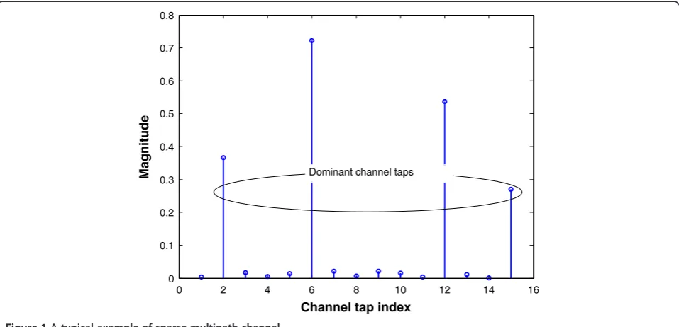
The demand for high-speed data services has been increasing as emerging wireless devices are widely spreading. Various portable wireless devices, e.g., smartphones and laptops, have generated rapidly, giving rise to massive data traffic [1]. Broadband transmission is an indispensable technique in the next-generation wireless communication systems [2,3]. The broadband channel is described by a sparse channel model in which multipath taps are widely separated in time, thereby creating a large delay spread [4-8]. In other words, most of channel coefficients are zero or close to zero, while only a few channel coefficients are dominant (large value). A typical example of sparse multipath channel is shown in Figure 1, where the number of dominant taps is four while the length is 16.

Traditional least mean square (LMS) is one of the most popular algorithms for adaptive system identification [9], e.g., channel estimation. LMS-based adaptive channel

estimation can be easily implemented due to its low computational complexity. In current broadband wireless communication systems, channel impulse response in time domain is often described by a sparse channel model, supported by a few large coefficients. The LMS-based adaptive channel estimation method never takes advantage of the channel sparse structure although its mean square error (MSE) lower bound has a direct relationship with finite impulse response (FIR) channel length. To improve the estimation performance, recently, many algorithms have been proposed to take advantage of the sparse nature of the channel. For example, based on the recent theory of compressive sensing (CS) [10,11], various sparse channel estimation methods have been proposed in [12-14]. Some of these methods are known to achieve robust estimation, e.g., sparse channel estimation using least-absolute shrink-age and selection operator [15]. However, these kinds of sparse methods have two potential disadvantages: one is that computational complexity may be very high, especially for tracking fast time-variant channels; the other is that training signal matrices for these CS-based sparse channel

* Correspondence:[email protected]

Department of Communications Engineering Graduate School of Engineering, Tohoku University, Sendai 980-8579, Japan

(2)

estimation methods are required to satisfy the restricted isometry property [16]. It was well known that designing these training matrices is a non-deterministic polynomial-time (NP)-hard problem [17].

In order to avoid the two detrimental problems of sparse channel estimation, a variation of the LMS algo-rithm with ℓ1-norm sparse constraint has been pro-posed in [18]. The ℓ1-norm sparse penalty is incorporated into the cost function of the conventional LMS algorithm, which results in the LMS update with a zero attractor, namely zero-attracting LMS (ZA-LMS)

andreweighted ZA-LMS(RZA-LMS) [18] which is

mo-tivated by the reweighted ℓ1-norm minimization recovery algorithm [19]. To further improve the estimation perform-ance, an adaptive sparse channel estimation method using

ℓp-norm LMS (LP-LMS) algorithm has been proposed [20]. However, there still exists a performance gap between LP-LMS and optimal sparse channel estimation. It is worth mentioning that optimal channel estimation is often de-noted by the sparse lower bound which is derived in The-orem 4 in Section 3.

Due to the fact that solving the LP-LMS algorithm is a non-convex problem, the algorithm cannot ob-tain an optimal adaptive sparse solution [10,11]. Hence, a computationally efficient algorithm is re-quired to obtain a more accurate adaptive sparse channel estimation.

According to the CS theory [10,11], solving the ℓ0 -norm sparse penalty problem can obtain an optimal sparse solution. In other words, ℓ0-norm sparse pen-alty on LMS algorithm is a good candidate to achieve more accurate channel estimations. These backgrounds motivate us to use the optimal ℓ0-norm

sparse penalty on LMS in order to improve the esti-mation performance.

In addition, since sparse LMS-based channel estima-tion methods have a common drawback of sensitivity to scaling of random training signal, it is very hard to choose a proper learning rate to achieve a robust estima-tion performance [21]. To solve this problem, we propose several improved adaptive sparse channel esti-mation methods using normalized LMS (NLMS) algo-rithm, which normalizes the power of input signal, with different sparse penalties, i.e.,ℓp-norm (0≤p≤1).

The contributions of this paper are described below. Firstly, we propose an improved adaptive sparse channel estimation method using ℓ0-norm least square error al-gorithm, termed as L0-LMS [22]. Secondly, based on algorithms in [18,20], we propose four kinds of improved adaptive sparse channel estimation methods using sparse NLMS algorithms. Thirdly, Cramer-Rao lower bound (CRLB) of the proposed adaptive sparse channel estimator is derived based on prior information of known positions of non-zero taps. Lastly, various simulation results are given to confirm the effectiveness of our proposed methods.

Section 2 introduces the system model and problem formulation. Section 3 discusses various adaptive sparse channel estimation methods using different LMS-based algorithms. In Section 4, computer simulation results for the MSE performance are presented to confirm the effect-iveness of sparsity-aware modifications of LMS. Concluding remarks are presented in Section 5.

2 System model and problem formulation

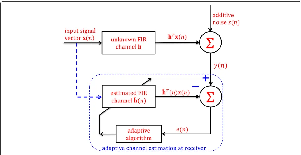
Consider a sparse multipath communication system, as shown in Figure 2.

0 2 4 6 8 10 12 14 16

0 0.1 0.2 0.3 0.4 0.5 0.6 0.7 0.8

Channel tap index Magnitude Dominant channel taps

(3)

The input signal x(t) and ideal output signal y(t) are related by

y tð Þ ¼hTxð Þ þt z tð Þ; ð1Þ

whereh= [h0,h1,…,hN− 1]TisN-length sparse channel

vector which is supported by K(K≪N) dominant taps, x(t) = [x(t),x(t−1),…,x(t−N+ 1)]Tis anN-length input signal vector ofx(t) andz(t) is an additive noise at time t. The objective of the LMS-type adaptive filter is to esti-mate the unknown sparse channel h usingx(t) andy(t). According to Equation 1, the nth channel estimation errore(n) is easily written as

e nð Þ ¼y tð Þ−h~Tð Þn xð Þ ¼t y tð Þ−h~Tð Þnxð Þt ; ð2Þ

at timet, whereh~ð Þn is the LMS adaptive channel estima-tor. It was worth noting that x(t) andy(t) are invariant as iterative times. Based on Equation 2, standard LMS cost function can be written as

L nð Þ ¼1 2e

2_{ð Þ}_n _: _ð₃_Þ

Hence, the updated equation of LMS adaptive channel estimation is derived as

~

hðnþ1Þ ¼h~ð Þn−μ∂L nð Þ

∂h~ð Þn ¼h~ð Þ þn μe nð Þxð Þt ; ð4Þ where μ is the step size of gradient descend. For later use, we define a parameter γmaxwhich is the maximum

eigenvalue of the covariance matrix R=E{x(t)xT(t)} of

input signal vector x(t). Here, we introduce Theorem 1 in relation to the step sizeμ. The detailed derivation can also be found in [21].

Theorem 1 The necessary condition of reliable LMS adaptive channel estimation is0<μ<2/γmax.

ProofAt first, the (n+ 1)th update coefficient vector

~

hðnþ1Þis written as

~

hðnþ1Þ ¼h~ð Þ þn μxð Þt e nð Þ

¼h~ð Þ þn μxð Þt y tð Þ−h~Tð Þn xð Þt : ð5Þ Assume thathis a real FIR channel vector; subtracting hfrom both sides in Equation 5, we can rewrite it as

~

hðnþ1Þ−h¼h~ð Þn−hþμxð Þt y tð Þ−h~Tð Þn xð Þt :

ð6Þ

By definingvð Þ ¼n h~ð Þn −hand according to Equation 1, Equation 6 can be rewritten as

vðnþ1Þ ¼vð Þ þn μxð Þt y tð Þ−hTxð Þt

þμxð Þt xT_{ð Þ}_t _h₋_xT_{ð Þ}_t _h~_{ð Þ}_n ¼vð Þ þn μxð Þt z tð Þ−μxð Þt xT_{ð Þ}_t _v_{ð Þ}_n ¼ðI−μxð Þt xTð Þt Þvð Þ þn μxð Þt z tð Þ:

ð7Þ

(4)

from the other, thenx(t) andz(t) are also independent, i.e., E{x(t)z(t)} = 0. Taking the expectation for both sides in Equation 7, we can obtain

Efvðnþ1Þg ¼E_ðI−μxð Þt xT_{ð Þ}_t _Þ_v_{ð Þ}_n_þ_E_f_μx_{ð Þ}_t _{z t}_{ð Þ}_g ¼I−μExð Þt xT_{ð Þ}_t _E_f_v_{ð Þ}_n_{g þ}_E_f_μx_{ð Þ}_t _{z t}_{ð Þ}_g ¼ðI−μRÞEfvð Þn g;

ð8Þ

The necessary condition of the reliable LMS adaptive channel estimation is given by

1−μλmax

j j<1; ð9Þ

whereλmaxdenotes the maximum eigenvalue ofR. Hence, to guarantee fast convergence speed and reliable updating of LMS in Equation 4, step sizeμshould be satisfied:

0<μ<2=λmax: ð10Þ □

3 (N)LMS-based adaptive sparse channel estimation

From Equation 4, we can find that the LMS-based channel estimation method never takes advantage of the sparse structure in channel vectorh. To get a better understand-ing, the LMS-based channel estimation methods can be expressed as

~

hðnþ1Þ ¼h~ð Þ þn Adaptive error update: ð11Þ

Unlike the conventional LMS method in Equation 11, sparse LMS algorithms exploit channel sparsity by intro-ducing several ℓp-norm penalties to their cost functions with 0≤p≤1. The LMS-based adaptive sparse channel estimation methods can be written as

~

Equation 12 motivated us to introduce different sparse penalties in order to take advantage of the sparse structure as prior information. Here, if we analogize the updated equation in Equation 12 to the CS-based sparse channel estimation [10,11], one can find that more accurate sparse channel approximation is adopted, and then better esti-mation accuracy could be obtained and vice versa. The conventional sparse penalties are ℓp-norm (0 <p≤1) and

ℓ0-norm, respectively. Since ℓ0-norm penalty on sparse signal recovery is a well-known NP-hard problem, only theℓp-norm (0 <p≤1)-based sparse LMS approaches have been proposed for adaptive sparse channel estimation. Compared to conventional two sparse LMS algorithms (ZA-LMS and RZA-LMS), LP-LMS can achieve a better

estimation performance. However, there still exists a performance gap between the LP-LMS-based channel estimator and the optimal one. As the development of mathematics continues, a more accurate sparse approxi-mate algorithm toℓ0-norm LMS (L0-LMS) is proposed in [22] and analyzed in [23]. However, they never considered any application on sparse channel estimation. In this paper, the L0-LMS algorithm is applied in adaptive sparse chan-nel estimation to improve the estimation performance.

It is easily found that exploitation of more accurate sparse structure information can obtain a better estimation performance. In the following, we investigate sparse LMS-based adaptive sparse channel estimation methods using different sparse penalties.

3.1 LMS-based adaptive sparse channel estimation

The following are the LMS-based adaptive sparse channel estimation methods:

_ZA-LMS. To exploit the channel sparsity in time domain, the cost function of ZA-LMS [18] is given by

LZAð Þ ¼n

whereλZAis a regularization parameter to balance the estimation error and sparse penalty of~hð Þn . The corresponding updated equation of ZA-LMS is

~ function which is defined as

sgnð Þ ¼h

From the updated equation in Equation14, the function of its second term is compressing small channel coefficients as zero in high probability. That is to say, most of the small channel coefficients can be simply replaced by zeros, which speeds up the convergence of this algorithm.

RZA-LMS. ZA-LMS cannot distinguish between

zero taps and non-zero taps as it gives the same penalty to all the taps which are often forced to be zero with the same probability; therefore, its performance will degrade in less sparse systems. Motivated by the reweighted ℓ1-norm

(5)

reinforce the zero attractor which was termed as the RZA-LMS [18]. The cost function of RZA-LMS is given by

LRZAð Þ ¼n 1

where λRZA> 0 is the regularization parameter and εRZA> 0 is the positive threshold. In computer simulation, the threshold is set as

εRZA= 20 which is also suggested in [18]. The expressed in the vector form as

~

hðnþ1Þ ¼h~ð Þ þn μe nð Þxð Þt −ρRZA

sgn~hð Þn 1þεRZA~hð Þn

:

Please note that the second term in Equation16 attracts the channel coefficients~hið Þn ;i¼1;2;…;N whose magnitudes are comparable to 1/εRZAto zeros. _LP-LMS. Following the above ideas in [18],

LP-LMS-based adaptive sparse channel estimation method has been proposed in [20]. The cost function of LP-LMS is given by

LLPð Þ ¼n

whereλLP> 0 is a regularization parameter. The corresponding updated equation of LP-LMS is given as

~

_{L0-LMS (proposed)}. Considerℓ0-norm penalty on LMS cost function to produce a sparse channel estimator as this penalty term forces the channel tap values ofh~ð Þn to approach zero. The cost function of L0-LMS is given by

LL0ð Þ ¼n

whereλL0> 0 is a regularization parameter and ~

hð Þn

0denotesℓ0-norm sparse penalty function which counts the number of non-zero channel taps of ~

hð Þn . Since solving theℓ0-norm minimization is an NP-hard problem [17], to reduce computational complexity, we replace it with an approximate continuous function:

The cost function in Equation19can then be rewritten as

The first-order Taylor series expansion of exponential functione−βjh~ið Þnj_{is given as}

The updated equation of L0-LMS-based adaptive sparse channel estimation can then be derived as

~

whereρL0=μλL0. Unfortunately, the exponential function in Equation23will also cause high computational complexity. To further reduce the complexity, an approximation functionJh~ð Þn is also proposed to the updated Equation23. Finally, the updated equation of L0-LMS-based adaptive sparse channel estimation can be derived as

~

3.2 Improved adaptive sparse channel estimation methods

(6)

scaling of their training signalx(t). In other words, LMS-based algorithms are sensitive to signal scaling [21]. Hence, it is very hard to choose a proper step size μto guarantee stability of these sparse LMS-based algorithms even if the step size satisfies the necessary condition in Equation 10.

Let us reconsider the updated equation of LMS in Equation 4. Assuming that thenth adaptive channel esti-mator h~ðnþ1Þ is the optimal solution, the relationship between the (n= 1)th channel estimator h~ðnþ1Þ and input signalx(t) is given as

~

hT_ð_n_þ₁_Þ_x_{ð Þ ¼}_t _{y t}_{ð Þ}_; _ð₂₆_Þ

where y(t) is assumed to be ideal received signal at the receiver. To solve a convex optimization problem in Equation 26, the cost function can be constructed as [21]

C nð Þ ¼~hðnþ1Þ−h~ð ÞnTh~ðnþ1Þ−h~ð Þn

þξy tð Þ−h~Tðnþ1Þxð Þt ;

ð27Þ

where ξ is the unknown real-value Lagrange multiplier [21]. The optimal channel estimator at the (n+ 1)th update can be found by letting the first derivative of

C nð Þ ¼0: ð28Þ

Hence, it can be derived as

∂C nð Þ

∂h~ðnþ1Þ¼2

~

hðnþ1Þ−h~ð Þn

−ξxð Þ ¼t 0: ð29Þ

The (n+ 1)th optimal channel estimator is given from Equation 29 as

~

hðnþ1Þ ¼h~ð Þ þn 1

2ξxð Þt : ð30Þ

By substituting Equation 30 into Equation 26, we ob-tain

ξxT_{ð Þ}_t _x_{ð Þ ¼}_t ₂_{y t}_{ð Þ}₋_h~T_{ð Þ}_n _x_{ð Þ}_t _¼_{2e n}_{ð Þ}_; _ð₃₁_Þ

where e nð Þ ¼y tð Þ−h~Tð Þnxð Þt (see Equation 2) and the unknown parameterξis given by

ξ¼ 2e nð Þ

xT_{ð Þ}_t _x_{ð Þ}_t : ð32Þ

By substituting it to Equation 30, the updated equation of NLMS is written as

~

hðnþ1Þ ¼h~ð Þ þn μ₁ e nð Þxð Þt

xT_{ð Þ}_t _x_{ð Þ}_t ; ð33Þ

where μ1 is the gradient step size which controls the

adaptive convergence speed of NLMS algorithm. Based on the updated Equation 33, for better understanding, NLMS-based sparse adaptive updated equation can be generalized as

~

hðnþ1Þ ¼~h_{|fflfflfflfflfflfflfflfflfflfflfflfflfflfflfflfflfflfflfflfflfflfflfflfflfflfflfflfflfflfflfflfflfflfflfflfflffl{zfflfflfflfflfflfflfflfflfflfflfflfflfflfflfflfflfflfflfflfflfflfflfflfflfflfflfflfflfflfflfflfflfflfflfflfflffl}}ð Þ þn Normalized adaptive error update NLMS

þSparse penalty

|fflfflfflfflfflfflfflfflfflfflfflfflfflfflfflfflfflfflfflfflfflfflfflfflfflfflfflfflfflfflfflfflfflfflfflfflfflfflfflfflfflfflfflfflfflfflfflfflfflfflfflfflfflffl{zfflfflfflfflfflfflfflfflfflfflfflfflfflfflfflfflfflfflfflfflfflfflfflfflfflfflfflfflfflfflfflfflfflfflfflfflfflfflfflfflfflfflfflfflfflfflfflfflfflfflfflfflfflffl} sparse NLMS

;

ð34Þ

where normalized adaptive update term is μ1e(n)x(t)/xT

(t)x(t) which replaces the adaptive update μe(n)x(t) in Equation 4. The advantage of NLMS-based adaptive sparse channel estimation it that it can mitigate the scal-ing interference of trainscal-ing signal due to the fact that NLMS-based methods estimate the sparse channel by normalizing with the power of training signal x(t). To ensure the stability of the NLMS-based algorithms, the necessary condition of step sizeμ1is derived briefly. The

detail derivation can also be found in [21].

Theorem 2The necessary condition of reliable NLMS adaptive channel estimation is

0<μ₁<

E e nn ð Þh−~hð Þn Txð Þt =xT_{ð Þ}_t _x_{ð Þ}_t o

E e_f 2_{ð Þ}_n₌_xT_{ð Þ}_t _x_{ð Þ}_t _g : ð35Þ

Proof Since the NLMS-based algorithms share the

same gradient step size to ensure their stability, for sim-plicity, studying the NLMS for a general case. The updated equation of NLMS is given by

~

hðnþ1Þ ¼h~ð Þ þn μ₁e nð Þ xð Þt

xT_{ð Þ}_t _x_{ð Þ}_t ; ð36Þ

where μ1 denotes the step size of NLMS-type

algo-rithms. Denoting the channel estimation error vector as uð Þ ¼n h−h~ð Þn ; (n + 1)th update error u(n+ 1) can be written as

uðnþ1Þ ¼uð Þn −μ₁e nð Þ xð Þt

xTð Þ_t xð Þ_t : ð37Þ

(7)

Eu2ðnþ1Þ¼Eu2ð Þn −2μ₁E e nð Þu

To ensure the stable updating of the NLMS-type algo-rithms, the necessary condition is satisfying

Eu2ðnþ1Þ−Eu2ð Þn ¼−2μ1E Hence, the necessary condition of reliable adaptive sparse channel estimation isμ1satisfying the theorem in

Equation 35.

□

The following are the improved adaptive sparse channel estimation methods:

ZA-NLMS (proposed). According to the

Equation14, the updated equation of ZA-NLMS can be written as

~

_{RZA-NLMS (proposed)}. According to Equation16, the updated equation of RZA-NLMS can be written as

~ regularization parameter for RZA-NLMS. The threshold is set asεRZAN=εRZA= 20 which is also consistent with our previous research in [24-27]. LP-NLMS (proposed). According to the LP-LMS in

Equation18, the updated equation of LP-NLMS can be written as parameter, andεLPN> 0 is a threshold parameter. _{L0-NLMS (proposed)}. Based on updated the

equation of L0-LMS algorithm in Equation24, the updated equation of L0-NLMS algorithm can be directly written as been defined as in (25).

3.3 Cramer-Rao lower bound

To decide the CRLB of the proposed channel estimator, Theorems 3 and 4 are derived as follows.

Theorem 3For an N-length channel vectorh,ifμ sat-isfies 0 <μ< 2/λmax, then MSE lower bound of LMS adaptive channel estimator is B¼μP0N=ð2−μλminÞeO

N

ð Þ, where P0is a parameter which denotes unit power of gradient noise and λmin denotes the minimum eigen-value ofR.

ProofFirstly, we define the estimation error at the (n+ 1) th iterationv(n+ 1) as ent error function which includes channel estimation error and noise plus interference error. To derive the lower bound of the channel estimator, two gradient errors should be separated. Hence, assuming Γ(n) can be split in two terms: Γð Þ ¼n Γ~ð Þ þn 2wð Þn where Γ~ð Þ ¼n 2Rh~ð Þn−p denotes the gradient error and w(n) = [w0(n),w1(n), …,

wN − 1(n)]T represents the gradient noise vector [21].

(8)

vðnþ1Þ ¼vð Þ þn μxð Þt e nð Þ

where the covariance matrix can be decomposed as R=QDQH. Here, Q is an N×N unitary matrix while D= diag{λ1, λ2, …, λN} is an N×N eigenvalue diagonal matrix. We denote ~vð Þ ¼n QHvð Þn and w~ð Þ ¼n QHwð Þn as the rotated vectors, and Equation 46 can be rewritten as

~

vðnþ1Þ ¼ðI−μDÞ~vð Þn −μw~ð Þn: ð47Þ

According to Equation 47, the MSE lower bound of LMS can be derived as

B¼ lim

Since signal and noise are independent, hence, E

~

wT_{ð Þ~}_n _v_{ð Þ}_n

¼…¼Ew~T_{ð Þ~}_n _v_{ð Þ}_n_¼_{0 , and Equation}

48 can be simplified as

B¼ lim

For a better understanding, the first term a(n) in Equation 49 can be expanded as

According to Equation 50, Equation 49 can be further rewritten as noise power. For any overall channel, since the LMS adaptive channel estimation method does not use the channel sparse structure information, the MSE lower bound should be cumulated from all of the channel taps. Hence, the lower boundBLMSof LMS is given by

B¼X are eigenvalues of the covariance matrixRandλminis its

minimal eigenvalue.

□

Theorem 4 For an N-length sparse channel vector h which consists of K non-zero taps,ifμsatisfies0 <μ< 2/

λmax,then the MSE lower bound of the sparse LMS adap-tive channel estimatorisBS¼μP0K=ð2−μλminÞeOð ÞK .

(9)

BS¼ XN−1

i¼0;i∈Ω

bi¼ X

i∈Ω

μP0

2−μλi≥ X

i∈Ω

μP0

2−μλmin ¼ μK P0

2−μλmine Oð ÞK :

ð54Þ

□

4 Computer simulations

In this section, we will compare the performance of the proposed channel estimators using 1,000 independent Monte Carlo runs for averaging. The length of sparse multipath channel h is set asN= 16, and its number of dominant taps is set asK= 1, 2, 4, and 8. For simplicity, the number of dominant taps is written in the form of a set asKϵ{1, 2, 4, 8}. The values of the dominant channel taps follow the Gaussian distribution, and the positions of dominant taps are randomly selected within the length of h and is subjected to k kh 2₂¼1. The received signal-to-noise ratio (SNR) is defined as 10 log E0=σ2n

, where E0 = 1 is the received signal power and the noise power is

given byσ2

n¼10−SNR=10. Here, we compare their

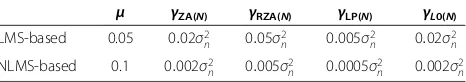
perform-ance with three SNR regimes: {5, 10, 20 dB}. All of the step sizes and regularization parameters are listed in Table 1. It is worth noting that the (N)LMS-based algorithms can exploit more accurate sparse channel information at higher SNR environment. Hence, all of the parameters are set at a direct ratio in relation with noise power. For example, in the case of SNR = 10 dB, the parameters of LMS-based algorithm are matched with the parameters which are given in [20]. Hence, the propose regulation parameter method can adaptively exploit the channel sparsity under different SNR regimes.

The estimation performance between the actual and estimated channels is evaluated by MSE standard which is defined as

MSEh~ð Þn ¼E h−h~ð Þn2₂

n o

; ð55Þ

where E{∙} denotes the expectation operator, and h and

~

hð Þn are the actual channel vector and its estimator, respectively.

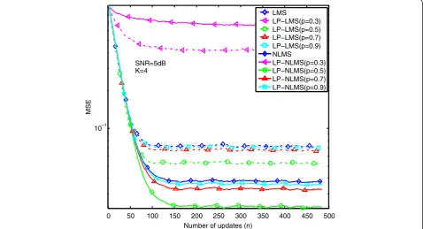
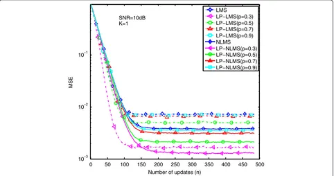
In the first experiment, we evaluate the estimation performance of LP-(N)LMS as a function ofpϵ{0.3, 0.5, 0.7, 0.9} which are shown in Figures 3, 4, 5, 6, 7, 8, 9, 10, 11, 12, 13, and 14 in three SNR regimes, i.e., {5, 10, 20 dB}. The parameter is set asεLP=εLPN= 0.05 which is

sug-gested in [20]. In the case of low SNR regime, e.g., SNR =

Table 1 Simulation parameters of (N)LMS-based algorithms

μ γZA(N) γRZA(N) γLP(N) γL0(N) LMS-based 0.05 0:02σ2

n 0:05σ2n 0:005σ2n 0:02σ2n

NLMS-based 0.1 0:002σ2

n 0:005σ2n 0:0005σ2n 0:002σ2n

0 50 100 150 200 250 300 350 400 450 500 10−1

Number of updates (n)

MSE

LMS

LP−LMS(p=0.3) LP−LMS(p=0.5) LP−LMS(p=0.7) LP−LMS(p=0.9) NLMS

LP−NLMS(p=0.3) LP−NLMS(p=0.5) LP−NLMS(p=0.7) LP−NLMS(p=0.9) SNR=5dB

K=1

(10)

5 dB,MSE performance curves are depicted in Figures 3, 4, 5, and 6, with different Kϵ{1, 2, 4, 8}. One can find that LP-(N)LMS algorithm is not stable if we setp= 0.3 because their estimation performances are even worse than the other cases, i.e.,pϵ{0.5, 0.7, 0.9}. In the case of

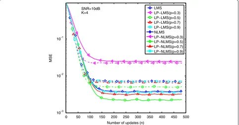
intermediate SNR regime, e.g., SNR = 10 dB, MSE per-formance curves are depicted in Figures 7, 8, 9, and 10, with differentKϵ{1, 2, 4, 8}. As shown in Figure 7, to estimate a very sparse channel (K= 1), the LP-(N)LMS algorithm with p= 0.3 can obtain a better estimation 0 50 100 150 200 250 300 350 400 450 500

10−1

MSE

LMS

K=2

Figure 4Performance comparison of LP-(N)LMS with differentp(SNR = 5 dB andK= 2).

0 50 100 150 200 250 300 350 400 450 500 10−1

MSE

LMS

K=4

(11)

performance than the others, i.e., p ϵ {0.5, 0.7, 0.9}. However, if K> 1, the LP-(N)LMS algorithm is no lon-ger stable as shown in Figures 8, 9, and 10, whose esti-mation performance is even worse than that in (N)LMS. In the case of high SNR regime, e.g., SNR = 20 dB,

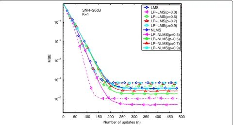
likewise, the LP-(N)LMS algorithm achieves a better es-timation performance than the others only whenK≤2 as shown in Figures 11 and 12. Hence, one can find that the stability of the LP-(N)LMS algorithm withp= 0.3 de-pends highly on both SNR andK. If the algorithm adopts 0 50 100 150 200 250 300 350 400 450 500

10−1

MSE

LMS

K=8

0 50 100 150 200 250 300 350 400 450 500 10−3

10−2 10−1

MSE

LMS

K=1

(12)

pϵ{0.5, 0.7, 0.9} as shown in Figures 3, 4, 5, 6, 7, 8, 9, 10, 11, 12, 13, and 14, fortunately, there is no obvious rela-tionship between stability and either SNR orK. In order to trade off stability and estimation performance of the LP-(N)LMS algorithm, it is better to set the value of the sparse penalty as p= 0.5. For one thing, the LP-(N)LMS

algorithm withp= 0.5 can always achieve a better esti-mation performance than the cases withpϵ{0.7, 0.9}. In another case, even though the LP-(N)LMS algorithm with p= 0.3 can obtain a better estimation performance in certain circumstances, its stability de-pends highly on SNR and K. Hence, in the following 0 50 100 150 200 250 300 350 400 450 500

10−3 10−2 10−1

MSE

LMS

K=2

0 50 100 150 200 250 300 350 400 450 500 10−3

10−2 10−1

MSE

LMS

K=4

(13)

simulation results, p= 0.5 is considered for LP-(N) LMS-based adaptive sparse channel estimation.

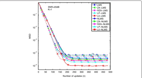
In the second experiment, we compare all the (N) LMS-based sparse adaptive channel estimation methods with different SNR regimes: {5, 20 dB} as

well as K ϵ {1, 8}, as shown in Figures 15, 16, 17, and 18, respectively. In the case of low SNR regime (e.g., SNR = 5 dB), the MSE curves show that NLMS-based methods achieve a better estimation performance than LMS-based ones as shown in Figure 15. Let us take ZA-NLMS and 0 50 100 150 200 250 300 350 400 450 500

10−3 10−2 10−1

MSE

LMS

K=8

0 50 100 150 200 250 300 350 400 450 500 10−5

10−4 10−3 10−2 10−1

MSE

LMS

K=1

(14)

ZA-LMS as examples. As shown in the figure, each per-formance curve of ZA-NLMS is much lower than that of ZA-LMS. That is to say, the proposed ZA-NLMS achieves a better estimation performance than the traditional ZA-LMS. Similarly, other proposed NLMS-type methods, i.e.,

RZA-NLMS and LP-NLMS, also achieve better estima-tion performances than their corresponding sparse LMS types. To further confirm the stability and effectiveness of our proposed methods, sparse (N) LMS-based estimation methods are also evaluated in 0 50 100 150 200 250 300 350 400 450 500

10−5 10−4 10−3 10−2 10−1

MSE

LMS

K=2

Figure 12Performance comparison of LP-(N)LMS with different_p(SNR = 20 dB and_K= 2).

0 50 100 150 200 250 300 350 400 450 500 10−4

10−3 10−2 10−1

MSE

LMS

K=4

(15)

the case of 20 dB as well as with different K, respectively.

As the SNR increases, the obvious performance advan-tages of NLMS-based methods are vanishing. Hence, compared with LMS-based methods, we can conclude

that NLMS-based methods not only work more reliably for unknown signal scaling, but also work more stably for noise interference, especially in low SNR environment.

In addition, the simulation results also show that (N) LMS-based methods have an inverse relationship with 0 50 100 150 200 250 300 350 400 450 500

10−4 10−3 10−2 10−1

MSE

LMS

K=8

0 50 100 150 200 250 300 350 400 450 500 10−2

10−1

MSE

LMS ZA−LMS RZA−LMS LP−LMS L0−LMS NLMS ZA−NLMS RZA−NLMS LP−NLMS L0−NLMS SNR=5dB

K=1

(16)

the number of non-zero channel taps. In other words, for a sparse channel, (N)LMS-based methods can achieve a bet-ter estimation performance and vice versa. Let us takeK= 1 and 8 as examples. In Figures 15 and 16, when the num-ber of non-zero taps isK= 1, performance gaps are bigger

than in the case whereK= 8, as shown in Figures 17 and 18. Hence, these simulation results also show that the esti-mation performance of adaptive sparse channel estiesti-mation is also affected by the number of non-zero channel taps. When the channel is no longer sparse, the performance of 0 50 100 150 200 250 300 350 400 450 500

10−2 10−1

MSE

K=8

Figure 16MSE versus the number of iterations (SNR = 5 dB and_K= 8).

0 50 100 150 200 250 300 350 400 450 500 10−5

10−4 10−3 10−2 10−1

MSD

K=1

(17)

these proposed methods will reduce to the performance of (N)LMS-based methods.

5 Conclusions

In this paper, we have investigated various (N)LMS-based adaptive sparse channel estimation methods by enforcing different sparse penalties, e.g.,ℓp-norm andℓ0 -norm. The research motivation originated from the fact that LMS-based channel estimation methods are sensi-tive to the scaling of random training signal and easily causing the estimation performance unstable. Unlike LMS-based methods, the proposed NLMS-based methods have avoided the uncertain signal scaling and normalized the power of input signal with different sparse penalties.

Initially, we proposed an improved adaptive sparse channel estimation method using ℓ0-norm sparse con-straint LMS algorithm and compared it with ZA-LMS, RZA-LMS, and LP-LMS. The proposed method was based on the CS background thatℓ0-norm sparse penalty can ex-ploit a more accurate channel sparsity.

In addition, to improve the robust performance and increase the convergence speed, we proposed NLMS-based adaptive sparse channel estimation methods using different sparse penalties, i.e., ZA-NLMS, RZA-NLMS, LP-NLMS, and L0-NLMS. For example, ZA-NLMS can achieve a better estimation than ZA-LMS. The proposed methods exhibit faster convergence and better performance which are confirmed by computer simulations under vari-ous SNR environments.

Competing interests

The authors declare that they have no competing interests.

Acknowledgements

The authors would like to thank Dr. Koichi Adachi of the Institute for Infocomm Research for his valuable comments and suggestions as well as for the improvement of the English expression of this paper. The authors would like to extend their appreciation to the anonymous reviewers for their constructive comments. This work was supported by a grant-in-aid for the Japan Society for the Promotion of Science (JSPS) fellows (grant number 24∙02366).

Received: 20 December 2012 Accepted: 28 July 2013 Published: 5 August 2013

References

1. D Raychaudhuri, N Mandayam, Frontiers of wireless and mobile communications. Proc. IEEE100(4), 824–840 (2012)

2. F Adachi, D Grag, S Takaoka, K Takeda, Broadband CDMA techniques. IEEE Wirel. Commun.12(2), 8–18 (2005)

3. F Adachi, E Kudoh, New direction of broadband wireless technology. Wirel. Commun. Mob. Com.7(8), 969–983 (2007)

4. WF Schreiber, Advanced television systems for terrestrial broadcasting: some problems and some proposed solutions. Proc. IEEE83(6), 958–981 (1995) 5. AF Molisch, Ultra wideband propagation channels: theory, measurement,

and modelling. IEEE Trans. Veh. Technol.54(5), 1528–1545 (2005) 6. Z Yan, M Herdin, AM Sayeed, E Bonek,Experimental study of MIMO channel

statistics and capacity via the virtual channel representation(University of Wisconsin-Madison, Technique report, 2007)

7. N Czink, X Yin, H Ozcelik, M Herdin, E Bonek, BH Fleury, Cluster characteristics in a MIMO indoor propagation environment. IEEE Trans. Wirel. Commun. 6(4), 1465–1475 (2007)

8. L Vuokko, VM Kolmonen, J Salo, P Vainikainen, Measurement of large-scale cluster power characteristics for geometric channel models. IEEE Trans. Antennas Propagat.55(11), 3361–3365 (2007)

9. B Widrow, SD Stearns,Adaptive Signal Processing(Prentice Hall, New Jersey, 1985) 10. E Candes, J Romberg, T Tao, Robust uncertainty principles: exact signal

reconstruction from highly incomplete frequency information. IEEE Trans. Inform. Theory52(2), 489–509 (2006)

11. DL Donoho, Compressed sensing. IEEE Trans. Inform. Theory52(4), 1289–1306 (2006) 0 50 100 150 200 250 300 350 400 450 500

10−5 10−4 10−3 10−2 10−1

MSE

K=8

(18)

12. WU Bajwa, J Haupt, AM Sayeed, R Nowak, Compressed channel sensing: a new approach to estimating sparse multipath channels. Proc. IEEE98(6), 1058–1076 (2010) 13. G Taubock, F Hlawatsch, D Eiwen, H Rauhut, Compressive estimation of doubly

selective channels in multicarrier systems: leakage effects and sparsity-enhancing processing. IEEE J. Sel. Top. Sign Proces.4(2), 255–271 (2010) 14. G Gui, Q Wan, W Peng, F Adachi,Sparse multipath channel estimation using

compressive sampling matching pursuit algorithm. The 7th IEEE Vehicular Technology Society Asia Pacific Wireless Communications Symposium (APWCS), Kaohsiung, 20–21 May 2010pp. 1–5

15. R Tibshirani, Regression shrinkage and selection via the Lasso. J. Roy. Stat. Soc. (B)58(1), 267–288 (1996)

16. EJ Candes, The restricted isometry property and its implications for compressed sensing. Comptes Rendus Mathematique346(9–10), 589–592 (2008)

17. MR Garey, DS Johnson,Computers and Intractability: a Guide to the Theory of NP-Completeness(W.H. Freeman & Co, New York, NY, 1990)

18. Y Chen, Y Gu, AO Hero,Sparse LMS for system identification. IEEE International Conference on Acoustics, Speech and Signal Processing (ICASSP), Taipei, 19–24 April 2009pp. 3125–3128

19. EJ Candes, MB Wakin, SP Boyd, Enhancing sparsity by reweighted ℓ1-minimization. J. Fourier Anal. Appl.14(5–6), 877–905 (2008)

20. O Taheri, SA Vorobyov,Sparse channel estimation withℓp-norm and reweightedℓ1-norm penalized least mean squares. IEEE International Conference on Acoustics, Speech and Signal Processing (ICASSP), Prague, 22–27 May 2011pp. 2864–2867

21. S Haykin,Adaptive Filter Theory, 3rd edn. (Prentice-Hall, Englewood Cliffs, 1996) 22. YT Gu, J Jin, S Mei,ℓ0-Norm constraint LMS algorithm for sparse system

identification. IEEE Signal Process. Lett.16(9), 774–777 (2009)

23. GL Su, J Jin, YT Gu, J Wang, Performance analysis ofℓ0norm constraint least

mean square algorithm. IEEE Trans. Signal Process.60(5), 2223–2235 (2012) 24. G Gui, W Peng, F Adachi,Improved adaptive sparse channel estimation based

on the least mean square algorithm. IEEE Wireless Communications and Networking Conference (WCNC), Shanghai, 7–10 April 2013pp. 3130–3134

25. G Gui, A Mehbodniya, F Adachi,Least mean square/fourth algorithm for adaptive sparse channel estimation. IEEE International Symposium on Personal, Indoor and Mobile Radio Communications (PIMRC), London, 8–11 September 2013. in press

26. G Gui, A Mehbodniya, F Adachi,Adaptive sparse channel estimation using re-weighted zero-attracting normalized least mean fourth. 2nd IEEE/CIC International Conference on Communications in China (ICCC), Xian, 12–14 August 2013. in press

27. Z Huang, G Gui, A Huang, D Xiang, F Adachi,Regularization selection method for LMS-type sparse multipath channel estimation, in 19th Asia-Pacific Conference on Communications (APCC), Bali, 29–31 August 2013. in press

doi:10.1186/1687-1499-2013-204

Cite this article as:Gui and Adachi:Improved least mean square algorithm with application to adaptive sparse channel estimation. EURASIP Journal on Wireless Communications and Networking

20132013:204.

Submit your manuscript to a

journal and beneﬁ t from:

7Convenient online submission 7Rigorous peer review

7Immediate publication on acceptance 7Open access: articles freely available online 7High visibility within the ﬁ eld

7Retaining the copyright to your article