R E S E A R C H
Open Access
A novel centralized algorithm for
constructing virtual backbones in wireless
sensor networks
Chuanwen Luo
1, Wenping Chen
1, Jiguo Yu
2, Yongcai Wang
1and Deying Li
1*Abstract
Finding the minimum connected dominating set (MCDS) is a key problem in wireless sensor networks, which is crucial for efficient routing and broadcasting. However, the MCDS problem is NP-hard. In this paper, a new approximation algorithm with approximation ratioH()+3 in timeOn2is proposed to approach the MCDS problem. The key idea is to divide the sensors in CDS intocoresensors andsupportingsensors. The core sensors dominate the supporting sensors in CDS, while the supporting sensors dominate other sensors that are not in CDS. To minimize the number of both the cores and the supporters, a three-phased algorithm is proposed. (1) Finding the base-core sensors by constructing independent set (denoted asS1), in which the sensors who have the largest|N
2(v)|
|N(v)| (number of two-hop neighbors over the number of one-hop neighbors) will be selected greedily intoS1; (2)
Connecting all base-core sensors inS1to form a connected subgraph, the sensors in the subgraph are called cores; (3) Adding the one-hop neighbors of the core sensors to the supporter setS2. This guarantees a small number of sensors can be added into CDS, which is a novel scheme for MCDS construction. Extensive simulation results are shown to validate the performance of our algorithm.
Keywords: Wireless sensor network, Virtual backbone, Connected dominating set, Unit disk graph
1 Introduction
Wireless sensor networks (WSNs) play a critical role in many areas, such as environmental monitoring, disaster forecast, etc [1]. A key problem in WSN is multi-hop communication, because the communication range of a individual sensor is generally limited. In multi-hop com-munication, any two sensors that are within the commu-nication range of each other are called neighbors, which can communicate to each other. Other sensors that are not within the communication range of each other and want to communicate, need intermediate sensors between them to forward their packets (for instance, sensory data [2,3] and image data [4,5]).
However, due to the broadcasting nature of the wireless communication, if there is not a specific routing path for packet forwarding, all neighbors are possible to become
*Correspondence:[email protected]
1School of Information, Renmin University of China, Zhongguancun Road,
100872 Beijing, People’s Republic of China
Full list of author information is available at the end of the article
intermediators for forwarding messages, which causes message floodingproblem. The key way to avoid flooding is to find a communication backbone, so that the packets are relayed by the backbone sensors to save energy for the other sensors.
If modeling the WSN into an undirected graph, the con-nected dominating set (CDS) [6–8] is one of the good choices to construct virtual backbone of the network, because the sensor nodes in the CDS form a connected subgraph to forward messages from other sensors.
However, forwarding message may run into collision, which introduces retransmissions and increases end-to-end delays. As the number of sensors in the CDS grows, the negative effect of retransmissions increases greatly. Hence, CDS with smaller number of sensors is highly desired, which leads to the problem of finding the CDS with the minimum number of sensors, i.e., the minimum connected dominating set (MCDS) problem. However, it has been proved that the MCDS problem is NP-hard [9]. Therefore, approximation algorithms become the focus of addressing the MCDS problem. The majority of proposed
algorithms in literatures follow a general two-phased approach [10–14]. In the first phase, a dominating set is constructed, and the sensors in the dominating set are called dominators. In the second phase, additional sen-sors are selected, called connectors. Together with the dominators, they induce a connected CDS topology.
In this paper, we design a three-phased approximation algorithm for the MCDS problem in WSNs. Firstly, we propose a novel method to construct an independent set S1for the graphGsuch that any pair of complementary sensor subsets forS1 is separated by exactly three hops. Secondly, sensors in S1 are connected by other sensors that are added intoCto form a subtree. The number of sensors inCis an even number, since any pair of comple-mentary sensor subsets inS1is separated by two sensors. A supporter setS2is constructed that neighbors ofS1∪C are added into S2. S1 ∪C∪S2 is connected dominated set. The performances of the proposed algorithms are thoroughly analyzed.
Our contributions are presented as follow:
• We propose a novel algorithm to generate the CDS and construct the virtual backbones in WSNs. • We analyze the performance ratio and time
complexity of our algorithm.
• We conduct extensive simulations to demonstrate the performance of the algorithms. Simulation results show that the algorithm generates CDS with smaller size than the state-of-the-art algorithms in [15].
The rest of the paper is organized as follows. Related work is reviewed in Section2. Our novel centralized algo-rithm for constructing a CDS is presented in Section3. The performance of the proposed algorithm is thoroughly analyzed in Section4. Section5gives the results of sim-ulations, which show the performance of the algorithm. Finally, we conclude this paper in Section6.
2 Related works
In this section, we review the classical algorithms for con-structing CDS. For more comprehensive approximation algorithms for CDS construction, one can refer to Du and Wan and Yu et al. [16,17]. Since the MCDS problem in unit disk graph is NP-hard, many algorithms are proposed to compute approximation solutions. CDS construction algorithms can be divided into distributed algorithms and centralized algorithms.
2.1 Distributed algorithms
In the case of distributed algorithms, each node in the network only knows the local information and commu-nicates with its neighbors. Recently, the popular meth-ods for constructing CDS are to firstly construct an maximal independent set (MIS), then a CDS is formed by connecting the nodes in the MIS, such as [7,8,11–13].
In [7], Wan et al. proposed an ID-based distributed algorithm to construct a CDS with the performance ratio 8|opt| −2, whereoptrepresents the minimum connected dominating set of the unit disk graph. In [8,11,12], some MIS-based algorithms are proposed and the first phase of these algorithms is to construct an MIS as shown in [7]. In the second phase of the algorithm in [8], Li et al. constructed a Steiner tree for connecting all nodes in MIS. The performance ratio of their algorithm is (4.8+ ln 5)|opt| +1.2. In [11] Min et al. improved the construc-tion of Steiner tree to decrease the size of connectors. Consequently, they proved that the approximation ratio of the proposed algorithm is 6.8. In [12], Wan et al. proved the approximation ratio of [7] is 7.333 and proposed a new approximation algorithm with ratio 6.389. In [13], Misra et al. proposed a heuristic algorithm, called collaborative cover, to obtain an MIS. After that, they constructed a Steiner tree with minimum number of Steiner nodes to obtain a small CDS. The size of the CDS they got is at most
(4.8+ln 5)|opt| +1.2.
2.2 Centralized algorithms
In the literature, Guha and Kuller [6] proposed the first approximation algorithm to construct an MCDS as a vir-tual backbone in a wireless network. They presented two centralized greedy algorithms for CDS construction with approximation factor 2H()+2 andH()+2 respec-tively, whereis the maximum degree of the graph. In [18], Ruan et al. proposed another centralized algorithm with the approximation factor ln+2. In [19], Fu et al. proposed a centralized algorithm for CDS construction with the time complexityOn2. Note thatcan be as many asO(n). Thus, the time complexity of the algorithm in [19] isOn3.
In [15], Al-Nabhan et al. proposed three similar cen-tralized algorithms to construct CDSs in wireless network with approximation factor of 5. These approximation algorithms outperform the existing state-of-the-art meth-ods. Their algorithm contains four phases. The first phase is to construct a special independent setS1and any pair of complementary subsets of S1 is separated by exactly three hops. The second phase is to compute an MDS for each disconnected component and all nodes in MDS form the setS2. The third phase is to connectS2nodes andS1 nodes. The fourth phase is to connect all nodes inS1.
Some other centralized CDS construction algorithms also exist in the literatures [20–23].
The MCDS has many applications in the special net-work models, such as ad hoc netnet-works [24, 25], energy harvest networks [26], battery-free networks [27], cogni-tive ratio networks [28], and others [29–31].
Fig. 1Sensor state transition of our algorithm. The transition conditions are as follows:ahas the largest value of|N|N2((vv))||;bexists a black neighbor;c
has a red neighbor but does not have black neighbor;dexists a yellow neighbor but does not have black or red neighbor;ehas the largest value of |N2(v)|
|N(v)| among all blue nodes, whereN2(v)andN(v)only contain white nodes;fbecomes connector;gexists a black neighbor;hhas the maximum number of yellow neighbors among all red nodes;Ihas a red neighbor but does not have black neighbor;Jbecomes connector
algorithms proposed in [15], extensive simulations are conducted, and the results show effectiveness of our algo-rithm. A preliminary version [32] was published in WASA 2017.
3 MCDS construction
3.1 Model
For simplicity, all sensors in WSN are randomly deployed in the two-dimensional plane. Assume that all sensors have the same transmission range in the network. The WSN is modeled as a unit disk graphG(V,E), whereVis the set of all sensors andErepresents the set of links in the network. If the Euclidean distance between any two sensors uandvis less than or equal to 1, then there is an undirected edgeeuv between these two sensors. Each
sensorv ∈ V has a unique ID. LetN(v)be the set of all neighbors ofvanddv= |N(v)|be the degree ofv. Denote =max{dv|∀v∈V}andNi(v)to be thei-hops neighbor
set ofv.
3.1.1 Connected dominating set (CDS)
A dominating set (DS) of a graphG = (V,E) is a sub-setV ⊆ V such that each node inV\V is adjacent to at least one node inV, and a connected dominating set (CDS) is a dominating set which also induces a connected subgraph.
3.1.2 Minimum connected dominating set (MCDS) problem
Given a graphG=(V,E), the minimum connected dom-inating set problem is to find the CDS inGsuch that the size of the CDS is minimized.
In this paper, we propose a novel approximation algo-rithm for solving the MCDS problem.
3.2 Algorithm overview
In this section, we overview the proposed approximation algorithm for the MCDS problem. The algorithm consists of three phases.
• In the first phase, we construct an independent setS1
(sensors inS1calledbase-cores) for the graph G such
that any pair of complementary sensor subsets inS1
is separated by exactly three hops, which differs from the construction process of the first phase in [15]. • In the second phase, we select connectors fromV\S1
to connect the base-core sensors inS1for obtaining a
subtree, called all sensors on the subtree ascores. • In the third phase, we construct a supporter setS2
such that neighbors ofS1∪Care added intoS2. S1∪C∪S2forms a CDS.
For an illustrative purpose, we employ the different colors to differentiate sensor states during the construc-tion process of our algorithm. Figure 1 shows the state transition process of sensors in the WSN.
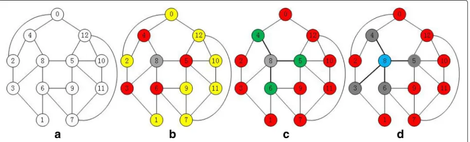
We illustrate the CDS construction process of our algo-rithm by Fig. 2, which is the same network example G(V,E)in [7]. Initially, all sensors are marked as white and each sensor has a unique ID, as shown in Fig.2a. In the first phase, we can know that node 8 has the largest value of ||NN2((vv))|| among all sensors in the graph. Hence, sensor 8 is colored black and all neighbors in N(8)are colored red and all sensors inN2(8)are colored yellow. As shown in Fig.2b, sensors 3, 4, 5, and 6 are colored red and sen-sors 0, 1, 2, 7, 9, 10, 11, and 12 are colored yellow. None of sensors become connector in the second phase since only one black sensor 8 is added into independent setS1. In the third phase, we need to select supporters (added intoS2) from red sensors to dominate all yellow sensors. For all red sensors, sensor 5 has the maximum number of yellow neighbors, then sensor 5 is marked green and its yellow neighbors 9, 10, 11, and 12 are colored red. After that, sensors 6 and 4 have the same number of yellow neighbors and the ID of sensor 6 is larger than sensor 4; therefore, sensor 6 is marked green and its yellow neigh-bors 1 and 7 are colored red. Then sensor 4 is marked green and sensors 0 and 2 are colored red. Finally, sensors with black and green form a CDS that contains sensors 4, 5, 6, and 8, as shown in Fig. 2c. Figure 2d shows a CDS (blue and black sensors) obtained by the algorithm in [12].
3.3 Independent setS1construction
In this section, we construct the setS1such that the hop distance between any two complementary sensor subsets inS1is exactly three hops. The details ofS1construction process as shown in the following steps.
First, a sensor v ∈ V with the largest value of |N|N2((vv))|| initiates theS1construction by coloring itself black. Then, the black sensor vdominates its neighbors inN(v) and all sensors in N(v)are marked red. After that, we color all sensors inN2(v)as yellow and all sensors inN3(v)are colored blue. Last, each blue sensorudeletes red sensors
from the setN2(u)and deletes yellow sensors from the set N(u).
Then select black sensor from the current blue sensors, for this purpose, the algorithm repeats the following steps, until no blue/white sensors is left in the graph.
We select a blue sensor vand color it black when the value of ||NN2((vv))|| is largest among all blue sensors. If more
than one sensor node have the same value of ||NN2((vv))||, then the algorithm selects the blue sensor with the maximum number of sensors inN(v). If more than one blue sensor have the same value of|N(v)|, then the algorithm selects the blue sensor with the highest ID value among these blue sensors.
After that, the algorithm executes the following opera-tions:
• All sensors inN(v)are colored red • All sensors inN2(v)are colored yellow • All sensors inN3(v)are colored blue
• Each blue sensoru deletes red sensors from the set
N2(u)and deletes yellow sensors from the setN(u)
The detail illustration as shown in Algorithm 1.
Algorithm 1S1Construction
1: Input:G(V,E) 2: Output:S1
3: Sets ofS1←ø;
4: All sensors inVare marked white;
5: Choose an initiatorv ∈V with the maximum ||NN2((vv))|| among all sensors inV;
6: Colorv=black;S1=S1∪ {v};
16: foreach blue sensorwdo
17: Delete red sensors from the set N2(w) and delete
yellow sensors from the setN(w);
18: end
19: Select blue sensor w with the largest value ||NN2((ww))|| among all blue sensors and setv=w;
20: Repeat line 4-17 until all sensors inVare black or red or yellow;
21: returnS1;
is composed of black sensors and any red sensor is defi-nitely dominated by a black sensor and any yellow sensor has two hops distance from a black sensor. We can prove that any pair of complementary sensor subsets ofS1is sep-arated by exactly three hops. The sensors in the setS1are calledbase-cores.
3.4 Connector setCconstruction
In this section, we propose a novel algorithm to find a set of connectors C such that S1 ∪ C forms a subtree.
Before we describe the algorithm, we introduce some terms and notations. For any subsetU ⊆ V, letq(U)be the number of connected components inG(U). The setU is initially equal toS1, and the initial value ofq(U)is|S1|. LetM = {e|e ∈ Eand the endpoints are red and yellow} andCbe the set of connectors. LetWbe the subset ofS1 such that any pair of sensors ofW is connected by other sensors inC.
To begin our algorithm, first, we select an arbitrary black sensors1 ∈ S1 to start selection of connectors and set W = {s1}. The algorithm repeats the following steps, until the conditionq(U)=1 is satisfied:
• Select a sensorsi∈Wsuch that there exists a sensor
sj∈N3(si)∩(S1−W)
• Select an edgeexy∈Msuch thatx∈N(sj)and
y∈N(si)
• Delete the edgeexyfromM, then sensors x and y are marked blue and added intoC
• For each yellow sensorw, ifw∈N(x)orw∈N(y), then it is marked red
• Execute operationsU=U∪ {u},U=U∪Cand
q(U)=q(U)−1
The detail illustration as shown in Algorithm 2.
After Algorithm 2 terminates, any two black sensors are connected by a path that consists of black sensors and blue sensors. That is, we obtain a subtree and all sensors on the subtree are calledcores.
3.5 Supporter setS2construction
After executing Algorithm 2, we have got a subtree over onS1∪C. However, there are still some yellow sensors not being dominated since they have two hops distance from black sensor or blue sensor.
In this section, we propose a novel greedy algorithm for acquiring a supporting set S2, in which the sensors are used to dominate remaining yellow sensors. Sensors in the setS2are calledsupporter.
LetRDbe the set{s|s ∈ V,Colors = red} andYLbe
the set{s|s ∈ V,Colors = yellow}. In each iteration, we
select a red sensors ∈ RDwith the maximum number of yellow sensors inN(s). If more than one red sensors
Algorithm 2ConnectingS1sensors
1: Input:G(V,E),S1
2: Output:C(The set of connectors)
3: Let U = S1, W,C ← ∅, M = {e|e ∈ E and the endpoints are red and yellow};
4: q(U)= |S1|;
5: Select arbitrary sensors1∈S1;
6: W =W∪ {s1};
7: whileq(U) >1do
8: Select a sensorsi ∈W such that there exists a sensor
sj∈N3(si)∩(S1−W);
have the same number of the yellow neighbors, then the algorithm selects the red sensor with the highest ID.
The algorithm repeats the following steps, until the conditionYL= ∅is satisfied:
• Select a red sensors∈Vwith the maximum number of yellow neighbors
• Sensors is marked green and its yellow neighbors in
N(s)∩YLare marked red
• Delete sensors ofN(s)∩YLfromYL
The detail illustration as shown in Algorithm 3.
Algorithm 3S2Construction
1: Input:G(V,E),S1,C
2: Output:S2
3: LetS2 ← ∅,RD = {s|s ∈ V,Colors = red},YL = {s|s∈V,Colors=yellow};
4: whileYL= ∅do
3.6 CDS construction
In this section, we propose our approximation algorithm for solving MCDS problem. The algorithm consists of four steps, and the first three steps correspond to Algo-rithms 1–3, respectively. The last step is to compute union of S1 , C, and S2. The detail illustration as shown in Algorithm 4.
After this algorithm terminates, we obtain a CDS that is union of S1 (black sensors), C (blue sensors), and S2 (green sensors). For a given graph G(V,E), we give the executing process of the Algorithm 4, as shown in Fig.3(a)-(d).
Algorithm 4CDSConstruction
Input:G(V,E) Output:CDS
step 1: Obtain independent set S1 by executing Algorithm 1;
step 2: Obtain connector set C by executing Algorithm 2;
step 3: Obtain supporter set S2 by executing Algorithm 3;
step 4:CDS=S1∪C∪S2; returnCDS;
4 Performance analysis
In this section, we analyze the performance ratio and time complexity of our algorithm. LetH(n) = ni=11i be the harmonic function and MCDS be an optimal CDS.
Lemma 1The set S1 found by Algorithm1is an inde-pendent set, and any pair of complementary sensor subsets of S1is separated by exactly three hops.
ProofWe use {s1,s2,· · ·,sk} to denote the set S1. Any two sensors si,sj ∈ S1 are not adjacent to each other according to the process of S1 construction by Algorithm 1. Therefore, the setS1is an independent set ofG.
LetTj= {s1,s2,· · ·,sj}andHj=(Tj,Ej)for any 1≤j≤
k. For arbitrary two sensorssi,sl ∈ Tj, an edge (si,sl) ∈
Ejif and only if their distance inGis three. We prove by
induction onjthatHjis connected. SinceH1contains a single sensor, it is connected obviously. Assume thatHj
is connected for 1 ≤ j ≤ k−1, when the sensorsj+1is marked black, according to the Algorithm 1, there exists si∈Ti(1≤i≤j) such that the distance betweensj+1and siinGis three, which means there exists an edge between
si andsj+1inHj+1. Due toHj is connected,Hj+1is also connected. Therefore,Hjis connected for any 1≤j≤k.
This implies that any pair of complementary subsets ofS1 is exactly three hops.
Lemma 2The CDS=S1∪C∪S2got by Algorithm4is a connected dominating set.
Proof According to lemma 1, we know that S1 is an independent set andS1∪Cis connected.
According to Algorithm 3, each sensor in S2 is adja-cent to at least one sensor inS1∪C. Therefore, the set CDS is connected. Since the distance between any sen-sor not inS1∪CandS1∪CinGis at most 2, all other sensors not in CDS are dominated by sensors in CDS according to the selection process of S2. Therefore, for any sensor v ∈ V, it belongs to the set CDS or has at least a neighbor inCDS, which meansCDSis a connected dominating set.
Lemma 3The size of S1is less than or equal to|MCDS|.
This lemma has been proved by lemma 2 in [15].
Lemma 4 The size of the set C obtained by Algorithm2 is at most2|MCDS| −2.
Proof LetS1be the set{s1,s2···,sk}. According to lemma
1, we obtain that auxiliary graph Hk over S1 is a tree. Hence,Hkcontainsk−1 edges. According to Algorithm 2,
any two endpoints of an edge inHkare two sensors inS1. Therefore, two connectors are added intoCto connect the two sensors.
Therefore, the size of setCis 2|S1| −2. By lemma 3, we get|C|is at most 2|MCDS| −2 .
Lemma 5The size of the set S2obtained by Algorithm3 is less than H()|MCDS|.
Proof For a sensorv∈MCDS, letPv be the sensors set
including v in which each sensor is dominated by v. According to Algorithm 3, when a red sensorvis marked green, all yellow neighbors ofvare dominated byv.
We will prove that the total number of sensors inPvfor
any nodevis at mostH().
Assume that when we pick a sensorvfromRDto add to S2,yyellow sensors turn to red. We obtain that each ofy yellow sensors spends at most 1y.
Assume that the number of yellow sensors is initially y0< inPv, and finally drops to 0. Letyjdenote the
num-ber of yellow sensors inPvafter stepj. Here, we assume
that some yellow sensors inPvare marked red at each step.
Therefore, the number of yellow sensors inPvdecreases
at each step. After the first step, the number of sensors which changed color isy0−y1. In thejth step, the num-ber of sensors that change color in setPvisyj−1−yj, and
the cost of each sensor which changed color is at most 1
0 100 200 300 400 500 600 700 800 900 1000
Fig. 3Let the transmission rangeRbe 250 m and deploy 100 sensors in the 1000*1000 m2detection area. The execution process of the Algorithm 4 as follows:aSelect a sensorsto startS1construction and sensorsis marked black.bAn independent setS1that contains four black sensors is constructed in step 1.cThe connector setCthat contains six blue sensors is constructed after executing step 2, and we obtain a subtree that contains allcores.dThe supporter setS2that consists of four green sensors is constructed in step 3, then we can obtain a CDS that consists of all black, blue, and green sensors
h 3–5, we obtain the following theorem.
Lemma 6The time complexity of Algorithm1is On2.
ProofAccording to Algorithm 1, we need|S1|iterations for obtaining the setS1. In the first iteration, we need at mostnsteps to choose a sensorvwith the largest value of ||NN2((vv))||fromV. Since any black sensor comes from blue sensor, we need at most n steps to select a black sen-sor from blue sensen-sors inith iteration. Therefore, the total number of black sensor selection over all iterations is On2 = O(n|S
1|), since |S1| < n, and we obtain that the time complexity of Algorithm 1 isOn2+O(n) = On2.
Lemma 7The time complexity of Algorithm2is On2.
ProofFirstly, we pick out all edges with a red endpoint and a yellow endpoint from setE. Therefore, the operation needs the running time ofO(|E|).
Secondly, due to the initial value of q(U) is |S1|, the number of iterations is less than|S1|by lemma 3. In the interior of the loop, first, we need|W|steps to select a sensorsi∈Wsuch that there exists a sensorsj∈N3(si)∩ (S1−W). The maximum value of|W|is equal to|S1|. Sec-ond, we select an edgeexy ∈ Mfor connectingsiandsj
such thatexyis composed of an endpointx∈N(si)and an
endpointy∈N(sj). Therefore, we need at most 2steps
to select edgeexy. Last, 2steps are needed for coloring
all sensors inN(x)∪N(y).
Therefore, the time complexity of Algorithm 2 isO(|E|+
(|W| +2+2)× |S1|)=O
n2.
Lemma 8The time complexity of Algorithm3is On2.
ProofWe need nsteps to pick out red sensors (added into RD) and yellow sensors (added into YL) from V. Algorithm 3 executes at most|YL|iterations. In a single iteration, due to the size ofRDis less thann, we need at mostnsteps a red sensorv∈RDwith the maximum num-ber of yellow neighbors among all sensors inRD. And at moststeps are needed to mark all yellow neighbors ofv. Therefore, the time complexity of Algorithm 3 isO((n+
+n)× |YL|)=O(n2), since|YL|<n.
We know that Algorithm 4 consists of four steps and the first three steps correspond to Algorithms 1, 2, and 3, respectively. The last step needs single time to compute the union ofS1,C, andS2. According to lemmas 6–8, we obtain the following theorem.
Theorem 2 The time complexity of Algorithm4is On2.
5 Simulation
In this section, we evaluate the performance of our algo-rithm through simulations. In the simulations,Nsensors
are randomly deployed in the two-dimension plane. All sensors are assumed to have the same transmission range R. Each experimental result is the average of 100 runs. We first evaluate how the network configuration, such as the number of the sensors, the transmission range, and the area of the deployment, impact on the size of CDS, as shown in Section5.1. After that, we compare the perfor-mance of our algorithm with the perforperfor-mance of the three algorithms (Approach I, Approach II, and Approach III) in [15], as shown in Section5.2. We used MATLAB R2013a for all simulations.
5.1 Impact of network configuration
In this section, we evaluate the impact of the different parameter settings on the size of CDS.
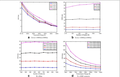
Firstly, Fig.4aillustrates the impact of the transmission rangeRon the size of CDS with different number of sen-sors. We randomly deployNsensors in a 1000×1000 m2 area, and measure the size of CDS when the transmis-sion range R varies from 200 to 500 m increased by 50 m. As shown in Fig.4a, we can observe that the size of CDS decreases as the transmission rangeRincreases. This is because when the transmission range becomes longer, the number of neighbors of sensors increase. That is to say, a backbone sensor is able to dominate more non-backbone sensors. When the transmission range R is large enough and the number of senors reaches to some number, the CDS size is almost same no mat-ter how big the number of sensors N is. It is because the some sensors can cover the whole detection area when the transmission range R is large enough. From Fig. 4a, when R= 500 m, the CDS sizes are almost the same. We can also find that the ratio of CDS size to the total number of sensors in the network decreases with the increasing of the density of network deploy-ment. For example, we fix R to 300 m, whenN = 100 andN = 500, the size of CDSs are 11.2 and 14.5, respec-tively, and the ratio of the former is 11.2% and the latter is 2.9%.
Secondly, we evaluate the impact of the number of sen-sorsNon the size of CDS with the different transmission rangeR. In the 1000×1000 m2monitor area, the number of sensorsN changes from 200 to 1200 sensors, we can find that the size of CDS increases with the number of sen-sors increasing whenR= 100 m and that the size of CDS levels off asRis more than 250 m, as shown in Fig.4b. We also obtain that, whenNis fixed, the size of CDS decreases more and more slowly with the increasing of the transmis-sion range when the transmistransmis-sion range reaches to some value.
b
a
d
c
Fig. 4The performance of our algorithm.aSize of CDS with a different value ofNwhenRvaries between 200 and 500 m.bSize of CDS with the different value ofRwhenNchanges from 200 and 1200 sensors.cSize of CDS with fixedR= 80 m whenNvaries between 200 and 1000 sensors.d
Size of CDS with fixedN=1000 sensors whenRchanges from 50 to 120 m
the impact of the number of sensorsNon the size of CDS in different detection areas, as shown in Fig.4c. When we fix the transmission range to 80 m and the number of sen-sorsN(from 200 to 1000), we can notice that the CDS size increases as the deployment area grows. Afterwards, we
evaluate the impact of the transmission range on the size of CDS in different detection areas, as shown in Fig.4d. When we fix the number of sensorsNto 1000 andR(from 50 to 120 m), we can notice that the CDS size increases as the deployment area grows.
a
b
b
a
Fig. 6Comparing results in the 600×600m2detection area.aThe average performance of four algorithms, whenN= 1000 sensors andRchanges from 50 to 120 m.bThe average performance of four algorithms whenR= 100m andNchanges from 100 to 1000 sensors
5.2 Performance evaluation
In this section, we compare the performance of our algorithm with the performance of the three algorithms (Approach I, Approach II, and Approach III) in [15]. To compare the performance of our algorithm with the three algorithms, we set the same value of the experiment parameters of our algorithm as the other three algorithms in [15].
Firstly, we give the comparison of the algorithms when the sensors are randomly deployed in the 300×300 m2 area, as shown in Fig. 5. When the number of sensors N = 1000 and the transmission rangeR is increased by 10 m from 50 to 120 m, we give the comparative results of the four algorithms in Fig.5a. The results show that the size of CDS got by our algorithm is always better than the other three algorithms as the transmission range becomes longer. And CDS sizes decrease with the transmission range increasing, which is because the transmission range
is bigger, the coverage area is larger, and the network area size is finite. Similarly, we fix the transmission rangeRto 50 m and changeNfrom 100 to 1000 sensors increased by 100. The comparative results in Fig.5billustrate that our algorithm outperforms the other three algorithms.
Secondly, for 600×600 m2monitor area, Fig.6shows the performance of the compared algorithms. If setting the number of sensorsN =1000 and changing the trans-mission range R between 50 and 100 m, our algorithm is better than the other three algorithms and the gap between the four results is getting smaller and smaller with increasing of the transmission range. By setting R= 100 m, Fig.6bgives the comparison in terms of CDS size through increasing the number of sensors from 100 to 1000. We can observe that our algorithm is still better than the other three algorithms.
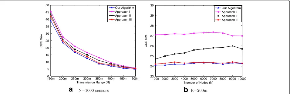
Finally, to better illustrate the superiority of our algorithm, we deploy the sensors 1000× 1000 m2 area
b
a
randomly, as shown in Fig.7. In Fig.7a, when the num-ber of sensorsN is fixed to 1000 andRvaries from 150 to 500 m, we can observe that our algorithm also outper-forms the other three algorithms in the larger detection area. And the size of CDS of the four algorithms tends to be stable when transmission range is big enough. Accord-ing to Fig.7b, if we setR=200 m and varyNfrom 1000 and 10,000, our algorithm still outperforms other three algorithms and the CDS sizes of the algorithms level off as the number of sensors increases, which means that our algorithm is also suitable in dense networks.
6 Conclusions
This paper proposes an approximation algorithm for the MCDS problem in wireless sensor networks. The key idea is to separate sensors in CDS intocoresensors and supportingsensors. The core sensors dominate the sup-porting sensors in CDS and some sensors are not in CDS, while the supporting sensors dominate remaining sen-sors that are not in CDS. Simulation results show that the algorithm generates CDS with smaller size than the state-of-the-art algorithms.
Abbreviations
CDS: Connected dominating set; DS: Dominating set; MCDS: Minimum connected dominating set; MIS: Maximal independent set; WSN: Wireless sensor network
Funding
This work was supported in part by the National Natural Science Foundation of China under Grants 11671400, 61672524; the Fundamental Research Funds for the Central University, and the Research Funds of Renmin University of China, 2015030273.
Authors’ contributions
CWL has contributed towards the algorithms, the analysis, and the simulations and written the paper. DYL has contributed towards the algorithms, and the analysis. As the supervisor of CWL, she has proofread the paper several times and provided guidance throughout the whole preparation of the manuscript. WPC, JGY, and YCW have revised the equations, helped writing the introduction and the related works, and critically revised the paper. All authors read and approved the final manuscript.
Competing interests
The authors declare that they have no competing interests.
Publisher’s Note
Springer Nature remains neutral with regard to jurisdictional claims in published maps and institutional affiliations.
Author details
1School of Information, Renmin University of China, Zhongguancun Road,
100872 Beijing, People’s Republic of China.2School of Information Science and Engineering, Qufu Normal University, Rizhao, 276826 Shandong, People’s Republic of China.
Received: 23 September 2017 Accepted: 27 February 2018
References
1. J Blum, M Ding, X Cheng, Applications of connected dominating sets in wireless networks. Handb. Comb. Optim.42, 329–369 (2004) 2. S Cheng, Z Cai, J Li, H Gao, Dataset from big sensory data in wireless
sensor networks. IEEE Trans. Knowl. Data Eng.29(4), 813–827 (2017)
3. J Li, S Cheng, Z Cai, J Yu, C Wang, Y Li, Approximate holistic aggregation in wireless sensor networks. ACM Trans. Sens. Netw.13(2), 1–24 (2017)
4. H Wu, Z Miao, Y Wang, M Lin, Optimized recognition with few instances based on semantic distance. Vis. Comput.31(4), 367–375 (2015) 5. H Wu, Z Miao, Y Wang, J Chen, C Ma, T Zhou, Image completion with
multi-image based on entropy reduction. Neurocomputing.159(7), 157–171 (2015)
6. S Guha, S Khuller, Approximation algorithms for connected dominating sets. Algorithmica.20(4), 374–387 (1998)
7. P-J Wan, KM Alzoubi, O Frieder, inProceedings IEEE, INFOCOM 2002. Twenty-First Annual Joint Conference of the IEEE Computer and Communications Societies, vol. 3. Distributed construction of connected dominating set in wireless ad hoc networks (IEEE, New York, 2002), pp. 1597–1604 8. Y Li, MT Thai, F Wang, C-W Yi, P-J Wan, D-Z Du, On greedy construction of
connected dominating sets in wireless networks. Wirel. Commun. Mob. Comput.5(8), 927–932 (2005)
9. BN Clark, CJ Colbourn, DS Johnson, Unit disk graphs. Discret. Math.
86(1-3), 165–177 (1990)
10. S Funke, A Kesselman, U Meyer, M Segal, A simple improved distributed algorithm for minimum cds in unit disk graphs. ACM Trans. Sens. Netw. (TOSN).2(3), 444–453 (2006)
11. M Min, H Du, X Jia, CX Huang, SC-H Huang, W Wu, Improving construction for connected dominating set with steiner tree in wireless sensor networks. J. Glob. Optim.35(1), 111–119 (2006)
12. P-J Wan, L Wang, F Yao, inDistributed Computing Systems, 2008. ICDCS’08. The 28th International Conference On. Two-phased approximation algorithms for minimum cds in wireless ad hoc networks (IEEE, Hang Zhou, 2008), pp. 337–344
13. R Misra, C Mandal, Minimum connected dominating set using a collaborative cover heuristic for ad hoc sensor networks. IEEE Trans. Parallel Distrib. Syst.21(3), 292–302 (2010)
14. Q Tang, Y-S Luo, M-Z Xie, P Li, Connected dominating set construction algorithm for wireless networks based on connected subset. J. Commun.
11(1), 50–57 (2016)
15. N Al-Nabhan, B Zhang, X Cheng, M Al-Rodhaan, A Al-Dhelaan, Three connected dominating set algorithms for wireless sensor networks. Int. J. Sens. Netw.21(1), 53–66 (2016)
16. D-Z Du, P-J Wan, Connected dominating set: theory and applications. Springer Sci. Bus. Media.77(2012)
17. J Yu, N Wang, G Wang, D Yu, Connected dominating sets in wireless ad hoc and sensor networks–a comprehensive survey. Comput. Commun.
36(2), 121–134 (2013)
18. L Ruan, H Du, X Jia, W Wu, Y Li, K-I Ko, A greedy approximation for minimum connected dominating sets. Theor. Comput. Sci.329(1-3), 325–330 (2004)
19. D Fu, L Han, L Liu, Q Gao, Z Feng, An efficient centralized algorithm for connected dominating set on wireless networks. Procedia Comput. Sci.
56, 162–167 (2015)
20. X Cheng, M Ding, D Chen, inProc. of International Workshop on Theoretical Aspects of Wireless Ad Hoc, Sensor, and Peer-to-Peer Networks (TAWN), vol. 2. An approximation algorithm for connected dominating set in ad hoc networks, (Washington, 2004)
21. H Du, W Wu, Q Ye, D Li, W Lee, X Xu, Cds-based virtual backbone construction with guaranteed routing cost in wireless sensor networks. IEEE Trans. Parallel Distrib. Syst.24(4), 652–661 (2013)
22. W Wang, B Liu, D Kim, D Li, J Wang, W Gao, A new constant factor approximation to construct highly fault-tolerant connected dominating set in unit disk graph. IEEE/ACM Trans. Netw. (TON).25(1), 18–28 (2017)
23. Y Shi, Z Zhang, Y Mo, D-Z Du, Approximation algorithm for minimum weight fault-tolerant virtual backbone in unit disk graphs. IEEE/ACM Trans. Netw.25(2), 925–933 (2017)
24. D Li, X Jia, H Liu, Energy efficient broadcast routing in static ad hoc wireless networks. IEEE Trans. Mob. Comput.3(2), 144–151 (2004) 25. Y Hong, D Bradley, D Kim, D Li, AO Tokuta, Z Ding, Construction of higher
spectral efficiency virtual backbone in wireless networks. Ad. Hoc. Netw.
25, 228–236 (2015)
27. T Shi, S Cheng, J Li, Z Cai, inThe 36th Annual IEEE International Conference on Computer Communications INFOCOM. Constructing connected dominating sets in battery-free networks (IEEE, Atlanta, 2017), pp. 1–9 28. J Yu, W Li, X Cheng, M Atiquzzaman, H Wang, L Feng, Connected
dominating set construction in cognitive radio networks. Pers. Ubiquit. Comput.20(5), 757–769 (2016)
29. J Yu, N Wang, G Wang, Constructing minimum extended
weakly-connected dominating sets for clustering in ad hoc networks. J. Parallel Distrib. Comput.72(1), 35–47 (2012)
30. S Cheng, Z Cai, J Li, Curve query processing in wireless sensor networks. IEEE Trans. Veh. Technol.64(11), 5198–5209 (2015)
31. Z He, Z Cai, S Cheng, X Wang, Approximate aggregation for tracking quantiles and range countings in wireless sensor networks. Theor. Comput. Sci.607, 381–390 (2015)