University of Tennessee, Knoxville
Trace: Tennessee Research and Creative
Exchange
Doctoral Dissertations Graduate School
8-2016
Face Centered Image Analysis Using Saliency and
Deep Learning Based Techniques
Rui Guo
University of Tennessee, Knoxville, [email protected]
This Dissertation is brought to you for free and open access by the Graduate School at Trace: Tennessee Research and Creative Exchange. It has been
Recommended Citation
Guo, Rui, "Face Centered Image Analysis Using Saliency and Deep Learning Based Techniques. " PhD diss., University of Tennessee, 2016.
To the Graduate Council:
I am submitting herewith a dissertation written by Rui Guo entitled "Face Centered Image Analysis Using Saliency and Deep Learning Based Techniques." I have examined the final electronic copy of this dissertation for form and content and recommend that it be accepted in partial fulfillment of the requirements for the degree of Doctor of Philosophy, with a major in Computer Engineering.
Hairong Qi, Major Professor We have read this dissertation and recommend its acceptance:
Jens Gregor, Lynne Parker, Yulong Xing
Accepted for the Council: Dixie L. Thompson Vice Provost and Dean of the Graduate School (Original signatures are on file with official student records.)
Face Centered Image Analysis
Using Saliency and Deep Learning
Based Techniques
A Dissertation Presented for the
Doctor of Philosophy
Degree
The University of Tennessee, Knoxville
Rui Guo
August 2016
c
by Rui Guo, 2016 All Rights Reserved.
Acknowledgements
The past 5 years are full of memories with smiles and tears. Though only my name appears on the cover of the dissertation, it is definitely a great many people have contributed to its generation. I owe my gratitude to all those people who have made this dissertation possible and because of whom my graduate experience has been one that I will cherish forever.
My deepest gratitude is to my advisor, Dr. Hairong Qi. I have been amazingly fortunate to have an advisor who gave me the freedom to explore on my own, and at the same time the guidance to recover when my steps faltered. Dr. Qi taught me how to question thoughts and express ideas. Her patience and support helped me overcome many crisis situations and finish this dissertation. I am always lucky to have her around not only input her time to my research but always willing to guide me in the life. My childish and temper are always tolerant in her good heart. The lessons I learnt would benefit me here and forever. Meanwhile, I would like to thank my committee members, Dr. Jens Gregor, Dr. Lynn Parker and Dr. Yulong Xing. Their insights about research inspire me in many ways. I really appreciate the time they input to my whole dissertation and defense including how to name a research work. I learnt a lot from their broad view in the frontier of machine learning, computer vision and algorithms. The spirits of rigid learning have been planted in my heart.
The outcome of my current learning has a strong tie to the environment which is built in our lab. I have lots of unforgotten days spending with my colleagues Li He, Jiajia Luo, Zhibo Wang, Shuangjiang Li, Liu Liu, Austin Albright, Daniel Capilla,
Bryan Bodkin, Yang Song, Zhifei Zhang, Alireza Rahimpour, Ali Taalimi, Ying Qu and Chengcheng Li. Not only the supports and courage you gave to me, but also the friendship built in our group will be memorized. Once an AICIPer, always an AICIPer!
Last but not least, I would like to express my deepest appreciation to my parents and my wife, for their unconditional support and encouragement. Their dedication and love are always the biggest motivation for any of my achievements. They are the source of the continuous power to make me fearless in the endeavor. My lovely daughter Evelyn is my greatest achievement. Love you all forever!
Abstract
Image analysis starts with the purpose of configuring vision machines that can perceive like human to intelligently infer general principles and sense the surrounding situations from imagery. This dissertation studies the face centered image analysis as the core problem in high level computer vision research and addresses the problem by tackling three challenging subjects: Are there anything interesting in the image? If there is, what is/are that/they? If there is a person presenting, who is he/she? What kind of expression he/she is performing? Can we know his/her age? Answering these problems results in the saliency-based object detection, deep learning structured objects categorization and recognition, human facial landmark detection and multitask biometrics.
To implement object detection, a three-level saliency detection based on the self-similarity technique (SMAP) is firstly proposed in the work. The first level of SMAP accommodates statistical methods to generate proto-background patches, followed by the second level that implements local contrast computation based on image self-similarity characteristics. At last, the spatial color distribution constraint is considered to realize the saliency detection. The outcome of the algorithm is a full resolution image with highlighted saliency objects and well-defined edges.
In object recognition, the Adaptive Deconvolution Network (ADN) is implemented to categorize the objects extracted from saliency detection. To improve the system performance,L1/2 norm regularized ADN has been proposed and tested in different
applications. The results demonstrate the efficiency and significance of the new structure.
To fully understand the facial biometrics related activity contained in the image, the low rank matrix decomposition is introduced to help locate the landmark points on the face images. The natural extension of this work is beneficial in human facial expression recognition and facial feature parsing research.
To facilitate the understanding of the detected facial image, the automatic facial image analysis becomes essential. We present a novel deeply learnt tree-structured face representation to uniformly model the human face with different semantic meanings. We show that the proposed feature yields unified representation in multi-task facial biometrics and the multi-multi-task learning framework is applicable to many other computer vision tasks.
Table of Contents
1 Introduction 1
1.1 Saliency Based Object Detection . . . 2
1.2 Object Recognition Via Deep Learning . . . 3
1.3 Facial Landmark Detection via Low-rank Matrix Decomposition . . . 5
1.4 Deep Tree-structured Face: A Unified Representation For Multi-task Facial Biometrics . . . 6
1.5 Contributions . . . 7
1.6 Outlines . . . 8
2 Literature Review 9 2.1 Review On Salient Region Detection . . . 9
2.2 Deep Feature Learning Background . . . 13
2.2.1 Restricted Boltzmann Machine . . . 14
2.2.2 Principles of Convolutional Neural Network . . . 17
2.2.3 Adaptive Deconvolutional Network . . . 18
2.3 Low Rank Matrix Decomposition . . . 18
2.3.1 Mathematics of Low Rank Matrix Decomposition . . . 19
3 Saliency-based Object Detection 21 3.1 Saliency Region and Visual Saliency Analysis . . . 21
3.2 The Saliency Detection Methodology - SMAP . . . 23
3.2.2 The Fine Tuning Process: Local Contrast Calculation . . . 27
3.2.3 The Global Saliency Response: Color Distribution Constraint 29 3.2.4 Saliency Map Generation . . . 34
3.3 Experiments and Evaluation . . . 34
3.3.1 Human Visual Fixations Prediction . . . 35
3.3.2 Visual Saliency Evaluation with Extracted Attention View . . 36
3.3.3 Visual Comparison on Different Types of Images. . . 38
3.3.4 Quantitative Comparison on Image Segmentation Results . . . 39
3.4 Applications . . . 41
3.4.1 Automatic Graphcut Segmentation . . . 41
3.4.2 Image Retargeting . . . 43
3.4.3 Scene Depth Effect on Commercial DC . . . 44
3.5 Conclusion . . . 45
4 Object Recognition via L1/2 Norm Regularized ADN 46 4.1 Introduction . . . 46
4.2 Feature Learning Approach: Adaptive Deconvolutional Network . . . 48
4.2.1 Feature Learning through Adaptive Deconvolutional Network. 48 4.2.2 L1/2 Norm Regularization on Feature Learning . . . 50
4.2.3 Feature Vector Formulation and Classification . . . 52
4.3 Object Recognition viaL1/2 Norm Regularized ADN: Evaluation . . . 53
4.4 Case Study: Facial Expression Recognition viaL1/2 Norm Regularized ADN . . . 58
4.4.1 Visualization of the Learnt ADN and Layer-wise Comparison for Expression Recognition . . . 59
4.4.2 The Robustness of The Unsupervised Feature . . . 63
4.4.3 The Role of L1/2 Norm Regularization . . . 64
4.4.4 Effect of Multi-resolution . . . 66
4.4.6 Discussion . . . 68
5 Facial Feature Parsing and Landmark Detection via Low-rank Matrix Decomposition 70 5.1 Related Work . . . 70
5.2 Parsing Algorithm . . . 72
5.2.1 Matrix Decomposition by Low-rank Matrix Representation . . 72
5.2.2 Facial Image Representation . . . 73
5.2.3 Learning Process of Linear Transformation Matrix . . . 73
5.2.4 Post-process and Landmark Detection . . . 74
5.3 Experiments . . . 75
5.3.1 Experiment I: Qualitative Performance of Face Parsing . . . . 75
5.3.2 Experiment II: Quantitative Performance of Landmark Detection 77 5.4 Conclusion . . . 78
6 Deep Tree-structured Face: A Unified Representation for Facial Biometrics 80 6.1 Introduction . . . 80
6.2 Learning Tree-structured Face Representation . . . 82
6.2.1 Single-layer CNN Network Learning . . . 82
6.2.2 Tree-structured Face Representation via Semi-supervised Au-toEncoder . . . 85
6.3 Experiments . . . 89
6.3.1 FACES Dataset . . . 91
6.3.2 The Standard Tree-structured Representation Learning . . . . 92
6.3.3 Expression Recognition and Age Estimation Without Identity 93 6.3.4 Key Parameters Tuning . . . 94
6.4 Related Work . . . 96
6.4.1 Facial Biometrics . . . 96
6.5 Conclusion . . . 97
7 Conclusion 98
Bibliography 101
Appendix 115
List of Tables
3.1 Mutual information (MI) between the labeled patches in Fig. 3.1. All patches from the background share similar appearance with MI less than 3.704; the MI between the foreground and background patches are more than 5.25. . . 22 3.2 The quantitative evaluation of user experiment on extracted attention
view. . . 38 4.1 Statistics of the testing dataset from MSRA dataset B . . . 54 4.2 Recognition performance on MSRA saliency dataset. The comparison
approaches include PCA, SIFT and 5 layer CNN structure. . . 57 4.3 Performance comparison between saliency detection results, ground
truth object patch and entire image, as the training and testing inputs. 57 4.4 General L1 and L1/2 norm regularized ADN parameter setting and
layer-wised recognition performance. The last two rows contain the recognition accuracies forL1-ADN and L1/2-ADN respectively. . . 61
4.5 FER accuracy comparison. For LDA Yu and Yang (2001) (Linear Discriminant Analysis), 504 images are used for training, the rest are used as testing samples; for RI-LBP Shan et al. (2009) (Rotation-Invariant LBP), we use one-vs-all classification scheme and SVM as the classifier; for CNNPhung and Bouzerdoum (2009), we use one-vs-all classification scheme and percepton as the classifier. . . 63 4.6 Recognition accuracies comparison based on FER-2013. . . 63
4.7 L1/2 norm andL1 norm regularization comparison in image
reconstruc-tion . . . 65
4.8 Comparison between multiple input resolutions withL1/2-ADN and 4th layer features . . . 67
5.1 Testing results on FACES dataset . . . 78
6.1 The statistics of the FACES dataset . . . 91
6.2 Multi-task biometrics accuracies and average ranking . . . 93
List of Figures
3.1 The background patches have the self-similarity attribute . . . 22 3.2 The diagram of the proposed saliency detection system . . . 24 3.3 Gradient, spectral residualHou and Zhang (2007) and Gabor residual
of the image from Fig. 3.1. . . 25 3.4 Various division thresholds and the resulting Gabor residual images.
From left, the division threshold is set to 0.2 to 0.8 with 0.2 as the interval. 0.6 is the default setting. . . 26 3.5 The process of generating the background candidate pool . . . 26 3.6 Raw saliency map demonstration. From top row to the bottom:
original images, raw saliency maps. . . 29 3.7 A toy example to demonstrate the penalty effect. From left (a) original
image, (b) the CDC saliency map without spatial penalty, (c) the CDC saliency map with sigmoid-like penalty term. . . 33 3.8 Color distribution-constraint saliency map demonstration. Top row:
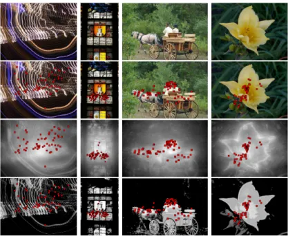
original images; bottom row: color distribution-constraint saliency maps. 33 3.9 Human visual fixation comparison. From top row, the original images,
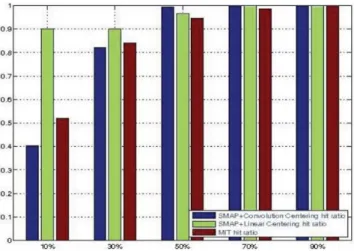
images with human fixation points (red dots), saliency maps fromJudd et al. (2009) with fixations and SMAP with fixations. . . 36 3.10 Quantitative comparison for human visual fixation prediction. Using
3.11 Visual saliency detection results. The red rectangles are extracted attention view areas calculated based on SMAP. The yellow rectangles are ground truth areas calculated based on ground truth mask with exhaustive search algorithm. . . 38 3.12 Precision and Recall curve comparison with the state-of-the-art
algo-rithms. SMAP is the proposed algorithm. . . 40 3.13 F-measure evaluation. . . 41 3.14 Saliency maps comparison. From the top row: original input images,
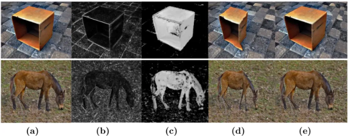
saliency maps generated by IT, SR, MZ, GB, CA, AC, LC, FT, HC, RC, LR and our proposed method SMAP. Columns (a)(b) demonstrate the color independent attribute which means the saliency map does not rely on color. Column(c) demonstrates the color uniqueness in multi-color environment. (d)(e) illustrate the scenario that the background contains texture information. Notice the red flower held by the toy bear in column(f), the proposed SMAP method is the only one detected efficiently the red part as the saliency part. In column (g), even in this extreme case, the gull is still detectable using the proposed algorithm. 42 3.15 Saliency map assisted image retargeting. (a) original images; (b)
default energy map by algorithm Avidan and Shamir (2007); (c) saliency map generated by the SMAP; (d) retargeting results by
Avidan and Shamir (2007); (e) retargeting results by the SMAP algorithm. . . 44 3.16 Saliency map assisted scene depth effect rendering. . . 45 4.1 Illustration of the Adaptive Deconvolutional Network (first two layers). 50 4.2 Feature vector formulation. The input is the projected first layer
4.3 Demonstrations of MSRA saliency dataset for object recognition. From top row to the bottom: Animal, Bird, Building, Car, Plant, Human and Traffic Sign. The demonstrated images are saliency detection results. All the images are normalized into the size of 256×256. . . 54 4.4 Learned filter kernels after training using 1000 saliency patches from
MSRA dataset. The numbers of kernels in each layer are 15, 50, 100 and 150 respectively. Each of them is of size 7×7. . . 55 4.5 Learned feature maps for each layer. The leftmost are feature maps
from layer 1 and the rightmost are feature maps from layer 4. Clearly, the fourth layer feature maps have already depicted object contours and detailed structures.. . . 56 4.6 Reconstructed images on image layer withM = 100 activations in the
fourth layer. . . 56 4.7 Expression databases illustration. The first row contains the six
expressions from FACES (Happy, Angry, Fearful, Sad, Disgusted and Neutral). The second row is the Lifespan database with two expressions. All the images are cropped based on region of interest for further usage. The last two rows contain the seven expressions from FER-2013 (Angry, Disgust, Fear, Happiness, Sadness, Surprise and Neutral). . . 59 4.8 Hierarchical features learnt by the proposed ADN architecture. Feature
generated by projecting the largest one activation from each layer back to the pixel space. From left, features learnt by layer 4 to layer 1. The activation from layer 4 has the receptive field covered the entire face. In the 3rd layer, features are acquired at the facial parts level (nose, eyes, mouse, etc.). Features in 2nd layer are mostly basic junction parts. In
the 1st layer, the primitive level Gabor-like features are learnt. The four-layer feature sets form the feature hierarchy. Noted that features are not in the original scale. . . 60
4.9 Demonstrations of the pooling locations on the images. The red blocks represent the pooling position at one channel. Notice that, most of the pooling position are coincident to the local landmarks on the face. . 62 4.10 Demonstrations of the learnt filter kernels and projected features from
3rdlayer activations to the image space on FER-2013 dataset. We have
15, 50 and 100 filters on each layer. . . 64 4.11 Demonstrations of the image reconstruction using 4th layer feature
ac-tivations. From left: original input image (gray value), reconstruction withL1/2 norm regularized ADN and the reconstruction withL1 norm
regularized ADN. From the figure, the left side nasolabial fold cannot be well reconstructed in the L1 norm regularized ADN. The MSE is
reported in Table 4.7. . . 65 4.12 Histogram of ∇xF (left) and ∇yF (right) by accumulated 50 facial
image feature maps on 4th layer. . . . . 66
5.1 Hand-labeled points on FACES image and the generated bounding rectangles for training. . . 76 5.2 Qualitative comparison on LFPW dataset. Noticed that, our results
received by testing on 500 non-occluded images. . . 76 5.3 Parsing map demonstration. The first row contains the original
input faces with Cascade Face Detector localized face regions. The second row contains the parsing map without transformation matrix T. The last row illustrates the parsing maps generated by the proposed algorithm. The parsing maps without T are polluted with unrelated pixels and the proposed method detects more regions on the facial components. . . 77 5.4 Landmark detection demonstration. The top row contains the images
6.1 Motivation of this work. Traditional facial image analysis treats the face recognition, expression recognition and age estimation separa-tively. We propose to jointly learn a unified representation for the face and use it in multi-task biometrics.. . . 81 6.2 Unsupervised CNN Filter Kernel Learning. The solid squares represent
centroids of clusters. . . 83 6.3 K-means learnt CNN filter kernels. k = 400, kernel size 9×9. Noticed
that, both of the Gabor-like kernels and QR code-like kernels emerge which are similar to the deep belief net first two layers kernels. . . 84 6.4 The structure of the semi-supervised AutoEncoder. We incorporate
labeling information in terms of cross-entropy errors to enforce dis-criminant feature learning. . . 89 6.5 The computation model demonstration. The super-pixels are
recur-sively combined to generate a tree-structured representation for the face image. Semi-supervised AutoEncoder is applied on each triplets to combine two super-pixels into one parent super-pixel. . . 90 6.6 FACES databases illustration. It contains the six expressions from
Angry, Disgust, Fear, Happy, Neutral and Sad. The two individuals represent persons from different aging group. . . 91 6.7 The recognition accuracies when tuning the key parameters. . . 95
Chapter 1
Introduction
Reasoning the surrounding environment and analyzing the situation from visual input is not only a fundamental function of human vision system but also a long-term striving goal of Artificial Intelligence and Computer Vision research. The implementation of this ambitious goal would greatly enhance the development in security surveillance and monitoring Thirde et al. (2006), robots visual navigation and planning Newman et al. (2006), abnormal event awareness in large scale social activity Thirde et al. (2006), computer-assisted medical image analysis for disease diagnosisMirota et al.(2009) and Internet image-based content search and acquisition engine design Li et al. (2009). Each of these applications requires a complicated reasoning in the image domain to distinguish the objects, background regions, geometric positions, color distributions, lighting, 3D structure and their correlated relationship. In the specific computer vision area, the image analysis is referred as to name the scene and objects located in the image. However, this over-simplified answer involves more challenges rather than a completed explanation. We are always pursuing to reach a higher level which is reasoning more semantic properties and structures from the image to enable the deep understanding of the objects, persons and their identities, expression and potential activities.
It is obvious that image analysis has multiple level requirements. Taking human vision generation processing as an example, in a short glance, human can rapidly locate the salient things in the whole perceptive field. After the locating, the refine process starts to recognize the attributes of the sensed objects and then estimate the activity and situation associated with objects. The whole process involves object detection, recognition and high level situation estimation. The straightforward assumption to tackle the term goal in image analysis is to decompose the long-term challenge into couple of highly correlated sub-tasks: object detection, recognition and activity analysis. Because of the huge spaces that the information spanned, the decomposition is quite reasonable to simplify the problem and meanwhile keeps it focus on the essential key points to answer the questions: is there anything interesting contained in the image? What are they? Who are they? And what are these people’s current status and potential activities? The completed answers to these questions spontaneously formulate the hierarchical procedure of human vision and neutron system corporately processing the visual input and so forth implementing the entire perceptive mechanism.
1.1
Saliency Based Object Detection
Human visual system has an incredible capability to implement the focus of attention mechanism. This judgment capability enables the visual system to rapidly and efficiently filter the important regions or objects out of the surrounding environment. Related research Grossberg (1995); Treisman and Gelade (1980) reveals that the behavior of the visual system is guided by both discriminant analysis and stimulusdriven process. Generally speaking, the global discriminant analysis is related to the human cognitive capability which is a learning process in memory and the neuron system. Millions of special patterns are learned and accumulated from personal experiences. Then classifiers formulated statistically are performed to locate the salient object from its surroundings. Comparatively, the local stimulus-driven
process only asks for short-term, small region response on the image Cheng et al.
(2015). Thus, the local contrast becomes the essential factor that determines the clear boundaries of salient objects Rutishauser et al.(2004).
In computer vision society, the concept of visual saliency originates from the visual importance. The extracted saliency regions are valuable to assist various image understanding tasks, including, for example, object detection, content-based segmentation, image retargeting, and object recognition. However, without any priorknowledge, accurately isolating the salient objects from complicated environment still challenges the vision researchers.
In this work, we propose a novel saliency detection strategy, SMAP, which combines both the discriminant method and the stimulus-driven approach to emulate the human vision mechanism. In the proposed framework, the Gabor spectral residual is firstly introduced to locate the proto-background region. Based on the similarity measurement between the computing patch and background patches in the candidate pool, the local contrast is computed to generate the raw saliency map. We also incorporate the color distribution constraint to produce the full-resolution saliency map. The proposed algorithm outperforms the state-of-the-art methods even in the clutter environment where the background patches are full of texture information.
1.2
Object Recognition Via Deep Learning
Our visual world exists in a dedicated complexity. To understand scenes, the computers or other intelligent machines have to classify or recognize a nature image into different categories first. That is also the essential task for the human vision system. To realize the recognition, the rich attributes of visual entries should be uniquely encoded into reasonable representations. Although the visual scene is continuous, to precisely entitle the image into functional and semantic group remains a huge challenge in computer vision.
The main advances in object recognition were achieved thanks to the improvement in object representation learning. The performance of recognition schemes is heavily depended on the choice of features where the visual input applied. The manually engineered representations combined with discriminatively trained models have been among the best performing paradigms for related object recognition problems. However, such feature engineering is labor-intensive and most of the times, is not reliable to extract discriminative features for labeling the input.
In the recent years, the Restricted Boltzmann Machines (RBM)Hinton(2002) and Convolutional Neutral Network (CNN)LeCun et al.(1998) have emerged as powerful machine learning models. Adaptive Deconvolutional Network (ADN) Zeiler et al.
(2011) is one of these edge-cutting deeply structured network. ADN is a multi-layer network which learns image representations that capture structure at all scales, from low-level edges to high-level object parts, in an unsupervised manner. Specifically, at each layer, the computing image/patch is decomposed into a linear combination of candidate features with sparse constraint. The inter-layer connection is in the form of max-pooling which responses the largest visual stimulus at a certain location. The original input image is always reconstructed at each layer. In this way, there is no information loss which exists in traditional Convolution Neutral Network, making the ADN more promising in hierarchical feature learning, and meanwhile benefiting the object recognition and categorization.
For ADN, despite the disentangling capability it has, we incorporate theL1/2norm regularization term instead of the originalL1 norm penalty to enhance the capability in feature learning. The proposed regularization forces the whole network to explore more sparse representations of the data and generate the hierarchical features with more discriminate information for object recognition.
1.3
Facial Landmark Detection via Low-rank
Ma-trix Decomposition
To better understand the facial activity, we conduct facial feature parsing and landmark detection to assist the better analysis.
In computer vision, facial feature parsing refers to the task that segmenting face images into different facial feature components, e.g., eyes, nose and mouth, and applying related information analysis. The study of facial parsing is an attractive area due to its importance in multiple applications, including human identity recognition, animation, demographic analysis Guo et al. (2013), facial image synthesis Amberg et al. (2007) and face image sketching Wang and Tang (2009). All of these applications ask for accurate segmentation and more requirements to the parsing algorithm – robust to expression, pose and illumination variations. Most existing works accomplish the task by localizing landmarks on the input face as the initial points, and then refine them pixel-wisely by classification or regression till completely segment the regions of interest out. As the prior knowledge, the template matching modelLiang et al.(2008) and graphic modelValstar et al.(2010) are applied to assist the parsing process.
In this work, we address the parsing problem from a new perspective and focus on facial feature detection from the face images instead of assigning label information for each pixel. Compared to previous methods, this detection-based approach is more efficient since it does not need to train the components descriptors piece-wisely. The facial features are treated as an entire set and can be detected at once. Specifically, our approach assumes a dataset of facial images with hand-labeled parsing map for each individual face. We emphasize that the alignment of all faces is not necessary. Clearly, the facial features contain discriminant shape, texture information, making them salient on the face region compared to the skin background. The intuitive idea to implement parsing is separating the salient components from the background. Our
considers the skin background as the matrix spanning in low dimension subspace and the facial features with their discriminant characteristics performed as sparse noise. We also apply face detector to assist the face localization. In order to enhance the matrix decomposition, we introduce a transformation matrixT to force the algorithm learn the unique facial features.
1.4
Deep Tree-structured Face: A Unified
Repre-sentation For Multi-task Facial Biometrics
Automatic facial image analysis has received considerable research interests due to its important role in computer vision and biometrics. As the key component, face feature is usually conducted under largely controlled environment and learnt for specific tasks which limit its discriminant capability in the unified representation. In this work, we present a novel deeply learnt tree-structured face representation to uniformly model the human face with different semantic meanings. The proposed feature is built from unsupervisedly learnt feature set, hierarchically combined region-by-region to generate a tree-structured representation. To enforce the semantic feature learning, we recursively apply semi-supervised AutoEncoder to incorporate label information which aims to disentangle the latent factors embedded in facial images. To validate the effectiveness of the proposed facial representation, we design comprehensive experiments based on FACES dataset which is considered as the most challenging one in terms of multi-factor overlapped. We show that the proposed feature yield unified representation in multi-task facial biometrics and the multi-task learning framework is applicable to many other computer vision tasks.1.5
Contributions
The primary objective of the research is to provide a face centered image analysis system which is strengthened by several advanced technologies in computer vision. To approach this goal, the major contributions of this work can be summarized in the listed details:
• The novel three-level saliency based object detection method SMAP is proposed. Included in the methodology, the first level of SMAP accommodates statistical methods to generate proto-background patches, followed by the second level that implements local contrast computation based on image self-similarity characteristics. At last, the spatial color distribution constraint is considered to realize the saliency detection. The outcome of the algorithm is a full resolution image with highlighted saliency objects and well-defined edges. Quantitative evaluation based on a popular benchmark shows that the proposed approach has higher detection accuracy and more consistent performance for various categories of images;
• A revised Adaptive Deconvolutional Network (ADN) is studied as an approach to implement the object recognition. To strengthen the capability of the original deep network, L1/2 norm regularization term is applied layer wisely to explore more discriminate features from images. Benefit from the new inference scheme of ADN, we visualize features learnt from each layer, and validate their roles in object recognition tasks. The hierarchical structure is evaluated based on the most popular benchmark dataset;
• It is the first time that low-rank matrix decomposition is introduced to solve the facial feature parsing problem. The proposed algorithm is detection-based method which is the initial work in this area. With the parsing results, we can easily extend the work to accomplish the facial landmark detection.
The high parsing accuracy guarantees the detection results receive competitive performance with the state-of-the-art;
• The unified deep face representation research is the first to propose the tree-structured face representation and implement it with designed semi-supervised AutoEncoder. It is proved to be effective in facial semantic learning. The proposed architecture is the first attempt to bridge the multi-task learning and deep learning to exploit latent feature learning for facial biometrics. It can be extended to many other computer vision applications.
1.6
Outlines
The organization of the dissertation is list as follows:
In chapter 2, the literature review is provided to introduce the state-of-the-art techniques in image analysis and facial biometrics included the salient object detection, object recognition deep learning neural network, so as the low-rank matrix decomposition theory. Chapter 3 explains the proposed salient object detection based on self-similarity. Chapter 4 introduces the L1/2 norm regularized Adaptive Deconvolutional Network as a novel approach for object recognition. As a case study, facial expression recognition using ADN is studied in this part. Chapter 5 discusses the further facial activity analysis in terms of facial feature parsing and landmark detection. The further discussion about a unified face representation for multi-task facial biometrics is in Chapter 6. The entire work is concluded in Chapter 7.
Chapter 2
Literature Review
2.1
Review On Salient Region Detection
Finding and localizing an object or objects from 2-dimensional image is a fundamental task in computer vision. Human localize a multitude of objects in their vision field with little effort despite the position, type, color, contrast, size, perspectives and even the translation, rotation of the objects. Indeed, humans can distinguish between more than 30,000 visual categories, and can detect objects in the span of a few hundred milliseconds. However, if we want to transfer the ability from human to the vision machines, the detection task becomes crucial and challenged for many reasons. Successful algorithms and systems should adopt the large range of uncertainties included appearance changes, non-rigid transformations, scaling variations and object obstructions. In other words, the universal model does not exist for the generic detection problem.
One of the most common solutions for object detection/localization is to slide a window across the image, and classify each such local window as target or background locations. This approach has been successfully used to detect rigid objects such as faces and cars and has even been applied to articulated objects such as pedestrians. However, natural weakness of this algorithm exists in several aspects: the window
size which is determined by object scaling is a hyper-parameter and different from case by case. Without pre-knowledge about the detecting object, it is hardly to choose the window size and trial it by random pick; another problem is that, the classification operation which is involved to distinguish the windowed patch belonging is a supervised process, which means for one category of objects, we should train a specific model for it. It is not feasible to use the technique to detect multiple classes of objects. The representative researches belonged to this approach includeDalal and Triggs(2005), GIST Oliva and Torralba(2001) and Bag-of-WordsFei-Fei and Perona
(2005) in object detection.
With the unsupervised preliminary, recent studies about object detection shift the focus to visual saliency. Visual saliency is the perceptual quality that makes a pixel, patch, object or person stand out to its neighborhood and thus attract human attention.
The study of the attention concept originates from human visual perception and neuro-psychology research. Researchers follow the methodology in Physiology to understand the eyes attention problem by analyzing the structure of human nervous system and brain. Although the mechanism to explain the operation of attention has not been completely understood, it shed light on computer vision groups that modeling the visual system could provide a rapid and reliable visual saliency detection. The pioneer work about attention theory was conducted by WilliamJames(2013), where the key point proposed emphasized on the psychological response rather than the physical aspect. Following this direction, BroadbentBroadbent(2013) established the filtering theory of attention and Deutsch Deutsch and Deutsch (1963) proposed the vision response selection principles. In 1960s, Hubel and Wiesels famous work on cats vision research revealed the relationship between visual receptive fields and cortexHubel and Wiesel(1962). At the same time, TreismanTreisman and Gormican
(1988) proposed a theory which combines selection from early and late visual processes into a comprehensive model, referred to as the Feature Integrated Theory (FIT). The FIT model guided the biological attention research from theoretical reasoning
into computational implementation. In 1985, Koch and Ullman proposed so-called bottom-up saliency Koch and Ullman (1987), leading to the discovery of the underlying mechanisms of neutral vision system, where the bio-inspired features were used to highlight the saliency location. With the advanced technologies in biology, recent works about attention explored deeper in the V1 and V4 areas of the optical nerves Li(2002).
In par with the biological attention research, the other direction focuses on the study of computational saliency models, where a number of models have been constructed by adapting the FIT theory. Niebur and Koch were the first to realize the computational saliency map Niebur and Koch (1998) in 1996. Itti and his group refined Kochs work by generating a master saliency map considering various features such as color, intensity, orientation, etc. Itti et al. (1998). Some later models added more specific features, such as the symmetry pattern Kootstra et al. (2008), texture contrastParkhurst et al.(2002), or motion informationItti et al.(2004) to the original structure. Saliency is also measurable in the frequency domain. In the spectral residual modelHou and Zhang(2007), saliency is described as the abnormal frequency from the smoothed FFT. This idea also incorporated natural image statistics related to the power law. In Achanta et al. (2009), the DOG filter was utilized to extract low-level features such as intensity and edges, which benefited the saliency evaluation. Notice that, most models mentioned above are stimulus-driven approaches where various features are crucial to determine the degree of saliency. The probability theory based on natural image statistics also gains popularity Itti and Baldi (2005); Zhang et al. (2008);Simoncelli and Olshausen (2001).
Among the aforementioned methods, the following algorithms are most state-of-the-art methods from different perspectives and mostly quoted in the peers works. The examination on properties of algorithms helps to reveal the advantages and limitations contained in each method.
image. Each feature is computed by a set of center-surround operations akin to visual receptive fields. Center-surround is implemented in the model as the difference between fine and coarse scales: The center is a pixel at scale c ∈ 2,3,4,, and the surround is the corresponding pixel at scale s = c+d, with d ∈ 3,4.. The across-scale difference between two maps is obtained by interpolation to the finer across-scale and point-by-point subtraction. Totally three domain feature maps are calculated, which are colors, intensities and orientations of the image. At higher level, the calculated feature maps are fused together to generate the final saliency map with winner-take all strategy. After the hierarchical blurring and downsampling, the net information remained from original image contains few details and caused the saliency maps very blurred.
In the approach of MZ Ma and Zhang (2003), a low-resolution image is created by averaging the quantized blocks of the image. Each block is then represented by a single averaged pixel value which is a simulation of low-pass filtering. The resulted image is fed into the local contrast computation. The contrast value is computed by calculating the summation of the Euclidean distances between the current pixel and the surrounding pixels in LUV color space. After normalization, the saliency map is generated by the contrast values.
In the approach of SR Hou and Zhang (2007), the spectral residual of the image is computed by subtracting a smoothed version of the FFT log-magnitude spectrum from the original log-magnitude spectrum. The author advocates that the spectral residual represent the response towards the visual stimulus. By setting a hand crafted threshold, the direct component of the spectrum is filtered out. The remaining spectrum is applied inverse FFT to transfer into image space resulted in the saliency map.
In the approach of HC Cheng et al. (2015), the pixel saliency value is defined as a global histogram-based contrast. As an improvement over HC-maps, spatial relations is incorporated to produce region-based contrast (RC) maps where the input image is firstly segmented into regions, and then assign saliency values to them. The saliency
value of a region is now calculated using a global contrast score, measured by the regions contrast and spatial distances to other regions in the image.
Although extraction of salient objects by the aforementioned algorithms receives reasonable results in some aspects, the reliable and accurate saliency estimation remains challenging for computer vision society. Inherited from the advantages of the modeling of human visual system, the bio-inspired algorithms attribute a strong ability to precisely locate the attentive points related to the early stage responses of the visual neurons toward the stimulus in the field of receptive. However, despite of its precision, these points usually occupy only the blurred regions rather than the clear objects in the image domain, making subsequent applications inconvenient. Other computational strategies adopting multi-feature model are suffering to find out a general model that encompasses all diverse variations in saliency detection. Once the model failed to represent the salient feature, the computational result may generate unexpected saliency values. In other words, the model-based strategies cannot receive consistent performance considering the various application scenarios.
2.2
Deep Feature Learning Background
Recently, deep feature learning has been applied to a wide range of application scenarios Bengio et al. (2013). The most attractive attribute of the deep learning is the machines (RBM, CNN and AutoEncoder etc.) that learn a hierarchy of features from primitively low level to semantically high level, and significantly outperform existing approaches in areas like object recognition, music categorization, OCR and speech recognition tasks Bengio et al. (2013). As the structure of the network goes deeper, the learning machines are able to assemble the local features into a composition, increasing the tolerance to translation, rotation and scaling Zeiler and Fergus (2014). Meanwhile, with the standard pipeline, the deep structure is able to build invariance to capture domain knowledge, such as the facial morphology in case of facial expression recognition Rifai et al.(2012).
2.2.1
Restricted Boltzmann Machine
One of unsupervised deep learning network successfully applied in machine learning is using the Restricted Boltzmann Machine (RBM). The RBM is firstly proposed as a random neutral network based on statistical mechanics. It is an undirected bipartite network involved the Energy-based Model (EBM) Bengio (2009), and naturally develops from Boltzmann Machine (BM). We introduce the mathematics of EBM and BM here to understand the fundamental concepts of them.
Energy-based Model And Hidden Variables
The main objective of statistical modeling is helping to capture the dependencies between variables. Once these dependencies are determined, a model can be easily applied to inference the unknown variables given the value of the known variables. However, the barrier always exists in many cases that distribution of the observation data is not pre-acquirable. Energy-based model is helpful to solve it by associating a scalar energy to each configuration of the variables. The problem converts to modify that energy function so that it fits the desirable requirements Bengio (2009). The energy-based model defines the energy function as,
P(x) = e
−Energy
Z (2.1)
where, the normalization factor Z is called the partition function. It defines as a sum running over the continuously input variable x,
Z =X
x
e−Energy(x) (2.2)
and describes physical prosperities of the statistical ensemble.
In many of the application cases, we do not directly observe the variable x, and instead it will be reflected by some non-observable variables. Introducing the hidden variable enriches the power of the model LeCun et al.(2006). Considering the model
comprises an observation x and a hidden variable h, the energy-based probabilistic models define the new probability distribution as,
P(x, h) = e
−Energy
Z (2.3)
Since x is observable, the marginal distribution is the main part we focus on
P(x) =X
h
e−Energy(x,h) (2.4)
By introducing a new notation, free energy, the Eq. 2.4 can be mapped to the similar one as Eq. 2.1,
P(x) = e −F reeEnergy(x) P xe−F reeEnergy(x) (2.5) with Z =P xe −F reeEnergy(x) and F reeEnergy(x) = −logX h e−F reeEnergy(x) (2.6)
The data log-likelihood gradient then becomes easily to calculate. Usingθto represent the parameters of the model, and taking the gradient on the both sides of Eq. 2.5, we can obtain, ∂logP(x) ∂θ =− ∂F reeEnergy(x) ∂θ + 1 Z X ˜ x e−F reeEnergy(˜x)∂F reeEnergy∂θ (x) =−∂F reeEnergy(x) ∂θ + X ˜ x P(˜x)∂F reeEnergy(˜x) ∂x˜ (2.7)
The mathematical expectation of the Eq. 2.7 can be written as,
EPˆ[ ∂logP(x) ∂θ ] =−EPˆ[ ∂F reeEnergy(x) ∂θ ] +EP[ ∂F reeEnergy(x) ∂θ ] (2.8)
On the right side of Eq. 2.8, the first term denotes the mathematical expectation taking over the training set, and the second term denotes expected value under the models distribution P. Therefore, to calculate the average log-likelihood gradient, we could sample from P and compute the free energy and then estimate with a Monte-Carlo way.
Boltzmann Machine
The Boltzmann Machine is a statistical model based on EBM and Restricted Boltzmann Machine is a particular form of Boltzmann Machine with more constraints on topological structure of the network. In the Boltzmann Machine, the energy function is formulated as,
Energy(x, h) = −bTx−cTh−hTW x−xTU x−hTV h (2.9)
The model parameters denoted by theta contain two parts: the biases bi and ci,
and the weightsWij,Uij andVij. Following the tractable form of Eq.2.7, the gradient
of the log-likelihood can be written as,
∂logP(x) ∂θ = ∂logP he −Energy(x,h) ∂θ − ∂logP x,he −Energy(x,h) ∂θ =− P 1 he−Energy(x,h) X h e−Energy(x,h)∂Energy(x, h) ∂θ +P 1 x,he−Energy(x,h) X x,h e−Energy(x,h)∂Energy(x, h) ∂θ =−X h P(h|x)∂Energy(x, h) ∂θ + X x,h P(x, h)∂Energy(x, h) ∂θ (2.10)
Noted that ∂Energy∂θ(x,h) is easy to compute by taking derivative on Eq. 2.5. Therefore, the main calculation becomes to implement a procedure to sample from
P(h|x) and sample fromP(x, h). Then we can obtain an unbiases stochastic estimator of the log-likelihood gradient. The problem is solvable by constructing an Monte
Carlo Markov Chain (MCMC) Andrieu et al. (2003) or Gibbs sampling Geman and Geman (1984). Recent work solved it using even shorter chains as Contrastive DivergenceHinton(2002), and this method has been adopted in training of Restricted Boltzmann Machine.
2.2.2
Principles of Convolutional Neural Network
Convolutional Neutral Network (CNN) is one of the most attractive models in the recent development of cognition research Bengio (2009);Bengio et al.(2013); Bengio
(2012). It was firstly inspired by the visual systems structure which is proposed by Hubel and Wiesel in their research of cats visual cortex Hubel and Wiesel (1962). Based on their works, the specific convolutional neural network efficiently reduces the complexity of back-propagation formed network. The CNN model based on the local connectivities between neurons and on hierarchically organized transformations of the image is efficient to obtain the translation invariant properties. Later on, researchers Alexander and Taylor improved the CNN theory and proposed the “improved perceptron which boosts the error-propagation algorithm Anthony and Bartlett(2009). LeCun followed-up with his idea to build up a new network structure trained with error gradient, obtaining the state-of-the-art performances in a variety of vision tasksLeCun et al. (1998,2010). In this dissertation, an alternative method Decovolutional Network which improves the CNN is adopted to implement the object recognition Zeiler et al. (2011); Zeiler and Fergus (2014). It inherits the advantages from the CNN but empowers with the unsupervised learning method which makes it be more suitable in discovering discriminate features from image space.
In general, the basic element of CNN is composed by a two-layer structure. The first layer is called the convolutional layer. At this layer, the previous layers feature maps are convolved with learnable kernels and put through the activation function to form the output feature map. Each output map may combine convolutions with multiple input maps. Another layer is called sub-sampling layer. A sub-sampling
layer produces downsampled versions of the input maps. If there are N input maps, then there will be exactly N output maps, although the output maps will be smaller. Usually, the max-pooling is taken as the default down-sample scheme. On each element, the sigmoid function is selected as the activation function which is helpful to acquire the translation invariant LeCun et al. (2006).
The completed CNN is constructed by multiple network elements with a super-vised perceptron as the output layer. The training method is following the traditional back-propagation algorithm to fine tune each parameter associated with every neuron.
2.2.3
Adaptive Deconvolutional Network
One particularly successful deep learning architecture is the Adaptive Deconvolutional Network (ADN) which offers appropriate features as well as the meaningful decompo-sition of the input images in multi-scaled levels Zeiler et al.(2011);Zeiler and Fergus
(2014). The principle underlying of ADN is that, the features on each layer are learnt directly by minimizing the reconstruction error of the input image under a sparsity constraint from an over-complete set of feature maps. Unlike the traditional deep machines, which use the lower level reconstruction as the input for subsequent layers, there is no missing information resulted in error accumulation for ADN because of the layer-wised reconstruction for the original input. The unique setting ‘switch’ enforces the network to retrieve the max-pooling route, and thus makes the learning and inference reversible between input and its layered features. Considering its properties and advantages in feature extraction, we are the first to evaluate the effectiveness of the ADN based feature hierarchy in capturing the expression changes in facial images.
2.3
Low Rank Matrix Decomposition
To complete the face centered image analysis, we still need to parse and locate the landmarks on human face to get better face image understanding after we fully
awareness that there is a person exist in the image. In the work, Low-rank Matrix Decomposition is adopted to assist the landmark points detection. We detail the assumption, problem formulation and related techniques in the following paragraphs.
2.3.1
Mathematics of Low Rank Matrix Decomposition
Suppose that we have a matrix A of size m×n with rank-r, where r min(m, n). In many engineering problems, the entries of the matrix are often corrupted by errors or noise, some of them could even be missing, or only a set of measurements of the matrix can be accessible instead of the matrix entries directly. In general, we model the observed matrix D to be a set of linear measurements on the matrix A, subject to noise and gross corruptions i.e., D=L(A) +η, whereLis a linear operator, and η
represents the matrix of corruptions. The problem is seeking to recover the genuine matrix A from D.
When to consider the case where L is the identity operator andηis a sparse matrix but whose non-zero entries can be practically unbounded. Since the rank r of A is unknown, the problem is to find the matrix of lowest rank that could have generated D when added to an unknown sparse matrix η. Mathematically, for an appropriate choice of parameterγ >0, we have the following combinatorial optimization problem to solve,
min
X,E rank(X) +γkEk0 subject to D=X+E (2.11)
where kk0 is the L0 norm.
Since the solving the above problem is NP-hard, one can alternatively solve it by another convex surrogate,
min
where kk∗ represents the matrix nuclear norm and is the best convex
approxima-tion to the rank funcapproxima-tion. kk1 represents L1 norm, and λ is a positive constant. In the paper proposed by Wright Wright et al. (2009), it shows that X and E can be perfectly recovered from Eq. 2.12
Chapter 3
Saliency-based Object Detection
3.1
Saliency Region and Visual Saliency Analysis
The hypothesis of human attention theory Li(2002);Reynolds and Desimone (2003) points out that the human visual system selectively analyzes the details of the partial image in the vision field but ignores the majority rest. From the general statistical analysis of natural images, we also found that, only a small portion of the single image contains richer information. The straightforward assumption is thus that the interesting part in vision has a corresponding relationship with the image region that has more information. All the other patches sharing similar appearance are treated as redundantZhang et al.(2008). The similar idea appeared in Gao’s workGao et al.
(2008). However, in his work, calculating the pre-defined clusters through a supervised method is neither efficient nor affordable with limited database or computational resource.
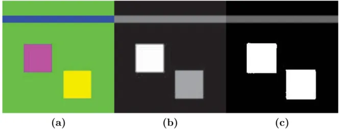
Take the image in Fig. 3.1 as an example where we manually select the patches from the foreground and background objects and calculate the mutual information between these patches, as shown in Table 3.1. We observe that the foreground patch (F in Fig.3.1) contains more distinct information than the background patches (R1,R2,Y1,Y2 in Fig. 3.1).
Figure 3.1: The background patches have the self-similarity attribute
Table 3.1: Mutual information (MI) between the labeled patches in Fig. 3.1. All patches from the background share similar appearance with MI less than 3.704; the MI between the foreground and background patches are more than 5.25.
M I F R1 R2 Y1 Y2 F 0 5.2585 6.2765 6.6777 6.8207 R1 5.2585 0 2.3687 2.5628 2.6069 R2 6.2765 2.3687 0 3.4273 3.3272 Y1 6.6777 2.5628 3.4273 0 3.7082 Y2 6.8207 2.6069 3.3272 3.7082 0
From the perspective of coding theory, one can always decompose the information of a static image into two parts, the prior knowledge and the abnormal propertiesHou and Zhang (2007). The former, most of time, is redundant and supposed to be suppressed by the coding process. The latter normally carries more distinctive information and therefore is the main focus of our research. There have been quite some efforts devoted to the search of the ‘disctinctive’ information in the image from different aspects. Until now, there has been no general model proposed that comprehensively describes the varieties of the whole image.
In this paper, we take the inverse approach to conventional saliency detection by first detecting the parts in the image that are not attractive. This approach would identify patches that do not contain distinctive attributes and share the self-similarity across the image, and thus are deemed as background candidates, referred to as the “proto-background”, as opposed to “proto-foreground” detected in conventional
approaches. Because of the self-similarity attributes, the accuracy of background detection is better appreciable than the detection of foreground salient parts.
Following the early selection of perception which outputs only the attentive points directly responding to outside stimulus, the subsequent biological process of human vision is the ‘refinement process’ that generates the perceptive field containing the semantic objects. To generate a perceptive field containing the salient objects with clear boundaries, local contrast is incorporated to evaluate the distinctiveness of each pixel. We define the local contrast as a feature-based similarity function between the evaluated patch and the proto-background patches.
Another plausible feature to describe saliency is the color distribution. It is commonly accepted that the color spatial distribution should be concentrated rather than scattered in the salient object that are attractive. As a global feature, the color distribution constraint also assists saliency representation to achieve a uniform and consistent performance among all images.
3.2
The Saliency Detection Methodology - SMAP
The goal of the proposed saliency detection system is to locate the potentially interesting foreground and to emulate the refinement process of eyes to better represent the saliency region and extract salient objects with full resolution. To achieve this goal, the pre-attentive process should filter the proto-background out of the image. Next, local contrast calculation is conducted to generate the raw saliency map. By adapting the observation that the color distribution of saliency object cannot be widely spread, we introduce the color distribution as a global constraint to assist the final detection. Correspondingly, the framework of the proposed system is composed of three parts and the saliency map produced would benefit in accuracy and uniform performance from both the local contrast and global constraint calculation.
Figure 3.2: The diagram of the proposed saliency detection system
3.2.1
The Local Stimuli Response: Proto-background
Detec-tion
Image analysis by Gabor filter bank is considered to resemble the perception in the human visual system Daugman (1985), where the quantitative response and tuning mechanism along the ventral stream of visual cortex is well modeled by the Gabor wavelets Riesenhuber and Poggio (1999). We thus adopt a set of Gabor filters at different scales and orientations to obtain the early attentive response. The sinusoidal Gaussian property enables the filters to produce the scale and position-tolerant features. The explicit form of the 2-dimensional Gabor filter in the spatial domain is described by,
G(x, y) = exp(−x 02+γ2y02 2σ2 ) cos( 2π λ x 0 ) (3.1)
where x0 =xcosθ+ysinθ and y0 =−xsinθ+ycosθ are the rotation factors of the Gabor filter controlled by the angle θ. σ is the standard deviation of the Gaussian envelope and γ is the spatial aspect ratio, which is fixed to γ = 0.3. λ represents the wavelength of the sinusoidal factor. Tuning ofλrelates to the change of the functional scale of the Gabor filter. Features in six orientations at five scales are computed. This
Figure 3.3: Gradient, spectral residual Hou and Zhang (2007) and Gabor residual of the image from Fig. 3.1.
filter bank is designed to acquire strong responses at locations where sharp stimulus matches at different orientations Guo et al. (2009).
In some natural scene images, the out-of-focus effect often causes blur at the object boundaries, introducing more uncertainties to the detection. To be more tolerant against the shift and out-of-focus effect, we measure the spectral residual from the Gabor spectrum. In one dimension, the spectral residual is calculated as,
R(f) = ln|G(f)| −hn∗ln|G(f)| (3.2) where hn = 1 3, 1 3, 1 3
works as an average filter, G(f) is the real part of the Gabor spectrum of the input image. The iF F T operation applied on R(f) would create an image with highlighted regions that relate to the early attentive points known as ‘abnormal’, or more specifically, the ‘proto-object’. Because the response is only analogous to the lowest level of early attention in the human visual system, it carries little semantic information but the maximum contrast caused by stimulus. Different from the classic spectral residual approach Hou and Zhang (2007), Gabor residual enriches the response in multiple orientations and scales. The texture details captured in the Gabor spectral space directly relate to the primitive receptive fields of the human vision. Fig.3.3indicates the relationship between the gradient and the Gabor residual. Clearly, Gabor residual has stronger response towards the gradient changes than conventional spectral residual.
Based on the proto-object calculated, the proto-background detection process is shown in Fig. 3.5. All the input images are uniformly rescaled to the size of 256×
Figure 3.4: Various division thresholds and the resulting Gabor residual images. From left, the division threshold is set to 0.2 to 0.8 with 0.2 as the interval. 0.6 is the default setting.
mask into quantized blocks of size 32 × 32. Counter-intuitively, the blocks with average intensity below a pre-defined threshold are selected as the proto-background regions. The selected blocks are stored in the Background Candidate Pool (BCP). The advantages of choosing the proto-background instead of the proto-object are two-fold. On one hand, the ‘redundancy’ property in the proto-background is more generic in different images. On the other hand, the scheme is robust to inaccurate detection. To balance the accuracy between the proto-objects and proto-background detection, we set the threshold as 0.6 times the average pixel intensity of the Gabor spectral residual image to select proto-background patches from the Gabor residual images. Higher threshold produces more precise proto-objects but poor proto-background estimation.
3.2.2
The Fine Tuning Process: Local Contrast Calculation
After locating the proto-background, the refining process is conducted to determine the whole area of the salient targets.
Almost all saliency algorithms utilize the color channels in different color spaces. The RGB color decomposition is the most frequently employed. Others argue Lab
provides better approximation as its components more closely match the human perception in lightness and chromaticsBorji and Itti(2012). Here we adopt theHSV
color space of Hue, Saturation and Value since it accommodates more traditional and intuitive color mixing models based upon how colors are organized and conceptualized in human vision Myers (1979). One favorable advantage received by using the HSV color decomposition is that, the saliency value calculated does not rely on any specific color.
Motivated by the color indexing technique, we incorporate the color moments to differentiate image patches based on their color feature. The color distribution of an image can be interpreted as the probability distribution. Thus, the moments are always proper choice to represent this distribution. We propose the first three momentsmean,standard deviationandskewness as the image color index. If the pixel value of a given color distribution is defined as pi in HSV color space, the moment
metrics can be defined as,
µ= µH µS µV , σ= (N1 PN i=1(p H i −µH)2) 1 2 (N1 PN i=1(p S i −µS)2) 1 2 (N1 PN i=1(p V i −µV)2) 1 2 s= (N1 PN i=1(p H i −µH)3) 1 3 (N1 PN i=1(p S i −µS)3) 1 3 (N1 PN i=1(p V i −µV)3) 1 3 (3.3)
where µ is the mean value of the distribution, N is the total amount of pixels in the distribution and the superscript represents different color channels. The three moments physically evaluate the average, variance and degree of asymmetry in color distribution. An image (or a patch I) is then easily characterized by totally 9 moments in the 3 color channels, i.e., I = (µ, σ, s)T.
The similarity measurement is defined as a sum function of the weighted difference between the moments of two distributions,H and I, i.e.,
dsim(H, I) =ω1T ·∆µ+ω
T
2 ·∆σ+ω
T
3 ·∆s (3.4) where ∆µ, ∆σand ∆srepresent the difference of moments between two distributions. Notice that the similarity comparison happens within the single image. The environmental condition is supposed to be unchanged. The weight vector is set to
{ωi = [1,1,1]}i=1,2,3, with nondiscriminant treatment on every element. Although these statistical representations vary significantly, they all help capture the color, edge features, repetitive patterns and complicated texture in a unified way, where the self-similarity is considered.
After acquiring the proto-background blocks, we subdivide these blocks into smaller 7×7 cells with 50% overlap. When evaluating the local contrast of a pixel
pi, the moments of 3×3 patch centered at pi are computed. The similarity between
pi and the background cells are calculated according to Eq. (3.4). We can obtain
a series of similarity values. The local contrast of pi is defined as the accumulated
minimal 128 similarity values between the computing patch Hi and the patches in
BCP. Hi is the 8-neighbor patch of pixel pi. The image texture with similar color
property and repetitive patterns is easily matched with the moment vectors inBCP, and thus receives a low contrast value. Apparently unique patches become visually salient since its similarity measurement based on BCP is rather strong. The image texture with similar color property and repetitive patterns is easily matched with the moment vectors in BCP, and thus receives a low contrast value. Apparently unique
Figure 3.6: Raw saliency map demonstration. From top row to the bottom: original images, raw saliency maps.
patches become visually salient since its similarity measurement based on BCP is rather strong.
The contrast values are normalized into the range [0 1]. The local contrast of the input image is treated as the raw saliency map Sraw. The figures in the 2nd row of
Fig. 3.6 illustrate the computed raw saliency maps Sraw.
3.2.3
The Global Saliency Response:
Color Distribution
Constraint
Although the Gabor spectral residual is quite effective to locate the saliency points in the receptive fields, the frequency domain method still suffers from one deficiency since the spatial distribution information is ignored. One of the possible drawbacks is that, in the clutter environment, the detected saliency parts may scatter all over the image.
The spatial distribution of a specific color may contribute significant information to the saliency detection. The concentration property of the saliency object indicates that, the wider a color distributes, the less possible it attracts human vision.
It is assumed that the color of the saliency object concentrates around a small region, making the small variance more attractive. Thus, the color distribution constraint indeed provides another important feature for saliency.
The Gaussian Mixture Model (GMM) is introduced to represent colors Liu et al.
(2011); Schwarz et al. (1978); Calinon et al. (2007). The image is treated as a data set with each pixel being a data point. A mixture model of c color clusters indexed byj,j = 1,2, ...c, is defined by a probability density function,
P(pi) =
X
c
P(j)P(pi|j) (3.5)
where pi is a vector represents the pixel value,P(j) is the prior and P(pi|j) denotes
the conditional probability density function. The image is modeled by a mixture of
c Gaussians of dimension d (for color images, d = 3). The parameters in Eq. (3.5) become P(j) =πj P(pi|j) =Φ(pi|µj,Σj) =q 1 (2π)d|P j| exp{−1 2(pi−µj) TΣ−1 j (pi−µj)} (3.6)
where{πj, µj,Σj}represent the prior, mean and covariance matrix of the color cluster
j in GMM respectively. The probability of a pixel pi assigned to the color cluster j
is defined as,
P(j|pi) =
P(j)Φ(pi|µj,Σj)
P(pi)
(3.7) The standard Expectation-Maximization (EM) algorithm is applied to solve the parameter estimation for mixed Gaussians iteratively. However, an obvious shortcoming of EM is that the optimal number of clusters in one image is unknown beforehand. To encode the image dataset with any fixed number of clusters will
result in either the deficiency in data modeling or parameter over-fitting. A traditional strategy to trade-off between optimizing data’s likelihood and minimizing the number of parameters used is the model selection. Bayesian Information Criterion (BIC) Schwarz et al. (1978) is then incorporated to tackle the estimation problem. The BIC score provides selection criteria to determine the optimal number of GMM clusters with the definition,
SBIC =−2L+nplog(N) (3.8)
whereL=PN
i=1log(P(pi)) andnp is the number of free parameters in the model. For
GMM,np = (j−1) +j(d+12d(d+ 1)). N is the total number of data points. L is the
log-likelihood function which measures the fitness of modeling on the data. nplog(N)
works as a penalty term to control the complexity of the model. Considering the goal of the algorithm is to segment the image based on color, we select the optimal number of color clusters as,
K = argmin c SBIC if c <= 6 d(argmin c SBIC)/2e if c > 6 (3.9)
where operator ‘de’ represents the smallest integer greater thanx. The selection of K
reaches a tradeoff between the optimal data fitting and reduced modeling complexity. We compute with a set of candidate Gaussians up to 15 color clusters and select the model parameters according to Eq.3.9.
The spatial distribution variance for each color cluster can then be interpreted as the weighted offset between each pixel position and the centroid. We penalize the offset if it is larger than half of the image range. The horizontal variance is formulated as Vh(c) = 1 |X|c X P(c|pi) λ· |xh−mh|2 1 + exp(−γ·width· |xh−mh|2) (3.10)