Distributed Asynchronous Online Learning for Natural Language Processing

Distributed Asynchronous Online Learning

for Natural Language Processing

Kevin Gimpel Dipanjan Das Noah A. Smith

Language Technologies Institute Carnegie Mellon Univeristy Pittsburgh, PA 15213, USA

{kgimpel,dipanjan,nasmith}@cs.cmu.edu

Abstract

Recent speed-ups for training large-scale models like those found in statistical NLP exploit distributed computing (either on multicore or “cloud” architectures) and rapidly converging online learning algo-rithms. Here we aim to combine the two. We focus on distributed, “mini-batch” learners that make frequent updates asyn-chronously(Nedic et al., 2001; Langford et al., 2009). We generalize existing asyn-chronous algorithms and experiment ex-tensively with structured prediction prob-lems from NLP, including discriminative, unsupervised, and non-convex learning scenarios. Our results show asynchronous learning can provide substantial speed-ups compared to distributed and single-processor mini-batch algorithms with no signs of error arising from the approximate nature of the technique.

1 Introduction

Modern statistical NLP models are notoriously expensive to train, requiring the use of generpurpose or specialized numerical optimization gorithms (e.g., gradient and coordinate ascent al-gorithms and variations on them like L-BFGS and EM) that iterate over training data many times. Two developments have led to major improve-ments in training time for NLP models:

• onlinelearning algorithms (LeCun et al., 1998; Crammer and Singer, 2003; Liang and Klein, 2009), which update the parameters of a model more frequently, processing only one or a small number of training examples, called a “mini-batch,” between updates; and

• distributedcomputing, which divides training data among multiple CPUs for faster processing between updates (e.g., Clark and Curran, 2004).

Online algorithms offer fast convergence rates and scalability to large datasets, but distributed computing is a more natural fit for algorithms that require a lot of computation—e.g., processing a large batch of training examples—to be done be-tween updates. Typically, distributedonline learn-ing has been done in asynchronoussetting, mean-ing that a mini-batch of data is divided among multiple CPUs, and the model is updated when they have all completed processing (Finkel et al., 2008). Each mini-batch is processed only after the previous one has completed.

Synchronous frameworks are appealing in that they simulate the same algorithms that work on a single processor, but they have the drawback that the benefits of parallelism are only obtainable within one mini-batch iteration. Moreover, empir-ical evaluations suggest that online methods only converge faster than batch algorithms when using very small mini-batches (Liang and Klein, 2009). In this case, synchronous parallelization will not offer much benefit.

In this paper, we focus our attention on asyn-chronous algorithms that generalize those pre-sented by Nedic et al. (2001) and Langford et al. (2009). In these algorithms, multiple mini-batches are processed simultaneously, each using poten-tially different and typically stale parameters. The key advantage of an asynchronous framework is that it allows processors to remain in near-constant use, preventing them from wasting cycles wait-ing for other processors to complete their por-tion of the current mini-batch. In this way, asyn-chronous algorithms allow more frequent parame-ter updates, which speeds convergence.

Our contributions are as follows:

• We describe a framework for distributed asyn-chronous optimization (§5) similar to those de-scribed by Nedic et al. (2001) and Langford et al. (2009), but permitting mini-batch learning. The prior work contains convergence results for asynchronous online stochastic gradient descent

for convex functions (discussed in brief in§5.2).

• We report experiments on three structured NLP tasks, including one problem that matches the conditions for convergence (named entity recognition; NER) and two that depart from the-oretical foundations, namely the use of asyn-chronous stepwise EM (Sato and Ishii, 2000; Capp´e and Moulines, 2009; Liang and Klein, 2009) for both convex and non-convex opti-mization.

• We directly compare asynchronous algorithms with multiprocessor synchronous mini-batch al-gorithms (e.g., Finkel et al., 2008) and tradi-tional batch algorithms.

• We experiment with adding artificial delays to simulate the effects of network or hardware traf-fic that could cause updates to be made with ex-tremely stale parameters.

• Our experimental settings include both indi-vidual 4-processor machines as well as large clusters of commodity machines implementing the MapReduce programming model (Dean and Ghemawat, 2004). We also explore effects of mini-batch size.

Our main conclusion is that, when small mini-batches work well, asynchronous algorithms of-fer substantial speed-ups without introducing er-ror. When large mini-batches work best, asyn-chronous learning does not hurt.

2 Optimization Setting

We consider the problem of optimizing a function

f :Rd→Rwith respect to its argument, denoted

θ = hθ1, θ2, . . . , θdi. We assume thatf is a sum

ofnconvex functions (hencefis also convex):1

f(θ) =Pn

i=1fi(θ) (1)

We initially focus our attention on functions that can be optimized using gradient or subgradient methods. Log-likelihood for a probabilistic model with fully observed training data (e.g., conditional random fields; Lafferty et al., 2001) is one exam-ple that frequently arises in NLP, where thefi(θ)

each correspond to an individual training exam-ple and theθ are log-linear feature weights. An-other example is large-margin learning for struc-tured prediction (Taskar et al., 2005;

Tsochan-1_{We use “convex” to mean convex-up when minimizing} and convex-down, or concave, when maximizing.

taridis et al., 2005), which can be solved by sub-gradient methods (Ratliff et al., 2006).

For concreteness, we discuss the architecture in terms of gradient-based optimization, using the following gradient descent update rule (for mini-mization problems):2

θ(t+1)←θ(t)−η(t)g(θ(t)) (2)

whereθ(t) is the parameter vector on thetth iter-ation,η(t)is the step size on thetth iteration, and

g:Rd→Rdis the vector function of first deriva-tives off with respect toθ:

g(θ) =D_∂θ∂f

1(θ),

∂f

∂θ2(θ), . . . ,

∂f

∂θd(θ)

E (3)

We are interested in optimizing such functions using distributed computing, by which we mean to include any system containing multiple processors that can communicate in order to perform a single task. The set of processors can range from two cores on a single machine to a MapReduce cluster of thousands of machines.

Note our assumption that the computation re-quired to optimize f with respect to θ is, essen-tially, the gradient vector g(θ(t)), which serves as the descent direction. The key to distribut-ing this computation is the fact that g(θ(t)) =

Pn

i=1gi(θ(t)), where gi(θ) denotes the gradient

offi(θ)with respect toθ. We now discuss several

ways to go about distributing such a problem, cul-minating in the asynchronous mini-batch setting.

3 Distributed Batch Optimization

Given p processors plus a master processor, the most straightforward way to optimizef is to par-tition the fi so that for each i ∈ {1,2, . . . , n},

g_i is computed on exactly one “slave” processor. LetIj denote the subset of examples assigned to

the jth slave processor (Sp

j=1Ij = {1, . . . , n}

and j 6= j0 ⇒ Ij ∩Ij0 = ∅). Processor j

re-ceives the examples in Ij along with the

neces-sary portions of θ(t) for calculating g_Ij(θ(t)) =

P

i∈Ijgi(θ

(t)_{). The result of this calculation is}

returned to the master processor, which calculates

g(θ(t)) = P

jgIj(θ

(t)_{) and executes Eq. 2 (or}

something more sophisticated that uses the same information) to obtain a new parameter vector.

It is natural to divide the data so that each pro-cessor is assigned approximatelyn/pof the train-ing examples. Because of variance in the expense

of calculating the differentg_i, and because of un-predictable variation among different processors’ speed (e.g., variation among nodes in a cluster, or in demands made by other users), there can be variation in the observed runtime of different pro-cessors on their respective subsamples. Each it-eration of calculating g will take as long as the longest-running among the processors, whatever the cause of that processor’s slowness. In comput-ing environments where the load on processors is beyond the control of the NLP researcher, this can be a major bottleneck.

Nonetheless, this simple approach is widely used in practice; approaches in which the gradient computation is distributed via MapReduce have recently been described in machine learning and NLP (Chu et al., 2006; Dyer et al., 2008; Wolfe et al., 2008). Mann et al. (2009) compare this frame-work to one in which each processor maintains a separateparameter vector which is updated inde-pendently of the others. At the end of learning, the parameter vectors are averaged or a vote is taken during prediction. A similar parameter-averaging approach was taken by Chiang et al. (2008) when parallelizing MIRA (Crammer et al., 2006). In this paper, we restrict our attention to distributed frameworks which maintain and update a single copy of the parameters θ. The use of multiple parameter vectors is essentially orthogonal to the framework we discuss here and we leave the inte-gration of the two ideas for future exploration.

4 Distributed Synchronous Mini-Batch

Optimization

Distributed computing can speed up batch algo-rithms, but we would like to transfer the well-known speed-ups offered by online and mini-batch algorithms to the distributed setting as well. The simplest way to implement mini-batch stochastic gradient descent (SGD) in a distributed computing environment is to divide each mini-batch (rather than the entire batch) among the processors that are available and to update the parameters once the gradient from the mini-batch has been computed. Finkel et al. (2008) used this approach to speed up training of a log-linear model for parsing. The interaction between the master processor and the distributed computing environment is nearly iden-tical to the distributed batch optimization scenario. WhereM(t)is the set of indices in the mini-batch

processed on iterationt, the update is:

θ(t+1)←θ(t)−η(t)P

i∈M(t)g_i(θ(t)) (4)

The distributed synchronous framework can provide speed-ups over a single-processor imple-mentation of SGD, but inevitably some processors will end up waiting for others to finish processing. This is the same bottleneck faced by the batch ver-sion in§3. While the time for each mini-batch is shorter than the time for a full batch, mini-batch algorithms make far more updates and some pro-cessor cycles will be wasted in computing each one. Also, more mini-batches imply that more time will be lost due to per-mini-batch overhead (e.g., waiting for synchronization locks in shared-memory systems, or sending data andθto the pro-cessors in systems without shared memory).

5 Distributed Asynchronous Mini-Batch

Optimization

An asynchronous framework may use multiple processors more efficiently and minimize idle time (Nedic et al., 2001; Langford et al., 2009). In this setting, the master sendsθand a mini-batchMkto

each slavek. Once slavekfinishes processing its mini-batch and returnsg_Mk(θ), the master imme-diately updatesθand sends a new mini-batch and the newθto the now-available slavek. As a result, slaves stay occupied and never need to wait on oth-ers to finish. However, nearly all gradient com-ponents are computed using slightly stale parame-ters that do not take into account the most recent updates. Nedic et al. (2001) proved that conver-gence is still guaranteed under certain conditions, and Langford et al. (2009) obtained convergence rate results. We describe these results in more de-tail in§5.2.

The update takes the following form:

θ(t+1)←θ(t)−η(t)P

i∈M(τ(t))g_i(θ(τ(t))) (5)

whereτ(t) ≤tis the start time of the mini-batch used for the tth update. Since we started pro-cessing the mini-batch at timeτ(t)(using param-etersθ(τ(t))), we denote the mini-batchM(τ(t)). If

τ(t) =t, then Eq. 5 is identical to Eq. 4. That is,

t−τ(t)captures the “staleness” of the parameters used to compute the gradient for thetth update.

Input: number of examplesn, mini-batch sizem, random seedr

θ`←θ;

seedRandomNumberGenerator(r);

whileconverged(θ) = falsedo g←0;

forj←1tomdo

k∼Uniform({1, . . . , n}); g←g+gk(θ`);

end

acquireLock(θ);

θ←updateParams(θ,g);

θ`←θ;

releaseLock(θ);

end

Algorithm 1:Procedure followed by each thread for multi-core asynchronous mini-batch optimization.θis the single copy of the parameters shared by all threads. The conver-gence criterion is left unspecified here.

of training examples. For example, for simple word alignment models like IBM Model 1 (Brown et al., 1993), only parameters corresponding to words appearing in the particular subsample of sentence pairs are needed. The error introduced when making asynchronous updates should intu-itively be less severe in these cases, where dif-ferent mini-batches use small and mostly non-overlapping subsets ofθ.

5.1 Implementation

The algorithm sketched above is general enough to be suitable for any distributed system, but when using a system with shared memory (e.g., a single multiprocessor machine) a more efficient imple-mentation is possible. In particular, we can avoid the master/slave architecture and simply start p

threads that each compute and execute updates in-dependently, with a synchronization lock onθ. In our single-machine experiments below, we use Al-gorithm 1 for each thread. A different random seed (r) is passed to each thread so that they do not all process the same sequence of examples. At com-pletion, the result is contained inθ.

5.2 Convergence Results

We now briefly summarize convergence results from Nedic et al. (2001) and Langford et al. (2009), which rely on the following assumptions: (i) The function f is convex. (ii) The gradients

g_iare bounded, i.e., there existsC > 0such that kg_i(θ(t))k ≤ C. (iii) ∃(unknown) D > 0such thatt−τ(t) < D. (iv) The stepsizesη(t) satisfy certain standard conditions.

In addition, Nedic et al. require that all func-tion components are used with the same

asymp-totic frequency (as t → ∞). Their results are strongest when choosing function components in each mini-batch using a “cyclic” rule: select func-tionfifor thekth time only after all functions have

been selected k−1 times. For a fixed step size

η, the sequence of function values f(θ(t)) con-verges to a region of the optimum that depends on η, the maximum norm of any gradient vector, and the maximum delay for any mini-batch. For a decreasing step size, convergence is guaranteed to the optimum. When choosing components uni-formly at random, convergence to the optimum is again guaranteed using a decreasing step size for-mula, but with slightly more stringent conditions on the step size.

Langford et al. (2009) present convergence rates via regret bounds, which are linear inD. The con-vergence rate of asynchronous stochastic gradient descent isO(√T D), whereT is the total number of updates made. In addition to the situation in which function components are chosen uniformly at random, Langford et al. provide results for sev-eral other scenarios, including the case in which an adversary supplies the training examples in what-ever ordering he chooses.

Below we experiment with optimization of both convex and non-convex functions, using fixed step sizes and decreasing step size formulas, and con-sider several values of D. Even when exploring regions of the experimental space that are not yet supported by theoretical results, asynchronous al-gorithms perform well empirically in all settings.

5.3 Gradients and Expectation-Maximization

task data n # params. eval. method convex? §6.1 named entity

recognition (CRF; Lafferty et al., 2001)

CoNLL 2003 English (Tjong Kim Sang and De Meulder, 2003)

14,987 sents.

1.3M F1 SGD yes

§6.2 word alignment (Model 1, both directions; Brown et al., 1993)

NAACL 2003 parallel text workshop (Mihalcea and Pedersen, 2003)

300K pairs

14.2M×2 (E→F + F→E)

AER EM yes

S6.3 unsupervised POS (bigram HMM)

Penn Treebank§1–21 (Marcus et al., 1993)

41,825 sents.

2,043,226 (Johnson, 2007)

EM no

Table 1: Our experiments consider three tasks.

0 2 4 6 8 10 12

84 86 88 90

Wall clock time (hours)

F1 Asynchronous (4 processors)

Synchronous (4 processors) Single−processor

Figure 1: NER: Synchronous mini-batch SGD converges faster in F1 than the single-processor

version, and the asynchronous version converges faster still. All curves use a mini-batch size of 4.

6 Experiments

We performed experiments to measure speed-ups obtainable through distributed online optimiza-tion. Since we will be considering different opti-mization algorithms and computing environments, we will primarily be interested in the wall-clock time required to obtain particular levels of perfor-mance on metrics appropriate to each task. We consider three tasks, detailed in Table 1.

For experiments on a single node, we used a 64-bit machine with two 2.6GHz dual-core CPUs (i.e., 4 processors in all) with a total of 8GB of RAM. This was a dedicated machine that was not available for any other jobs. We also conducted experiments using a cluster architecture running Hadoop 0.20 (an implementation of MapReduce), consisting of 400 machines, each having 2 quad-core 1.86GHz CPUs with a total of 6GB of RAM.

6.1 Named Entity Recognition

Our NER CRF used a standard set of features, fol-lowing Kazama and Torisawa (2007), along with token shape features like those in Collins (2002) and simple gazetteer features; a feature was in-cluded if and only it occurred at least once in train-ing data (total 1.3M). We used a diagonal Gaussian prior with a variance of1.0for each weight.

We compared SGD on a single processor to dis-tributed synchronous SGD and disdis-tributed asyn-chronous SGD. For all experiments, we used a fixed step size of0.01and chose each training ex-ample for each mini-batch uniformly at random from the full data set.3 We report performance by

3_{In preliminary experiments, we experimented with}

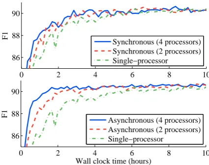
vari-0 2 4 6 8 10

86 88 90

F1 _{Synchronous (4 processors)}

Synchronous (2 processors) Single−processor

0 2 4 6 8 10

86 88 90

Wall clock time (hours)

F1

Asynchronous (4 processors) Asynchronous (2 processors) Single−processor

Figure 2: NER: (Top) Synchronous optimization improves very little when moving from 2 to 4 processors due to the need for load-balancing, leaving some processors idle for stretches of time. (Bottom) Asynchronous optimization does not require load balancing and therefore improves when mov-ing from 2 to 4 processors because each processor is in near-constant use. All curves use a mini-batch size of 4 and the “Single-processor” curve is identical in the two plots.

plotting test-set accuracy against wall-time over 12 hours.4

Comparing Synchronous and Asynchronous Algorithms Figure 1 shows our primary result for the NER experiments. When using all four available processors, the asynchronous algorithm converges faster than the other two algorithms. Er-ror due to stale parameters during gradient com-putation does not appear to cause any more

varia-ous fixed step sizes and decreasing step size schedules, and found a fixed step size to work best for all settings.

tion in performance than experienced by the syn-chronous mini-batch algorithm. Note that the dis-tributed synchronous algorithm and the single-processor algorithm make identical sequences of parameter updates; the only difference is the amount of time between each update. Since we save models every ten minutes and not every ith update, the curves have different shapes. The se-quence of updates for the asynchronous algorithm, on the other hand, actually depends on the vagaries of the computational environment. Nonetheless, the asynchronous algorithm using 4 processors has nearly converged after only 2 hours, while the single-processor algorithm requires 10–12 hours to reach the sameF1.

Varying the Number of Processors Figure 2 shows the improvement in convergence time by using 4 vs. 2 processors for the synchronous (top) and asynchronous (bottom) algorithms. The ad-ditional two processors help the asynchronous al-gorithm more than the synchronous one. This highlights the key advantage of asynchronous al-gorithms: it is easier to keep all processors in constant use. Synchronous algorithms might be improved through load-balancing; in our experi-ments here, we simply assignedm/pexamples to each processor, wheremis the mini-batch size and

pis the number of processors. Whenm=p, as in the 4-processor curve in the upper plot of Figure 2, we assign a single example to each processor; this is optimal in the sense that no other scheduling strategy will process the mini-batch faster. There-fore, the fact that the 2-processor and 4-processor curves are so close suggests that the extra two pro-cessors are not being fully exploited, indicating that the optimal load balancing strategy for a small mini-batch still leaves processors under-used due to the synchronous nature of the updates.

The only bottleneck in the asynchronous algo-rithm is the synchronization lock during updating, required since there is only one copy of θ. For CRFs with a few million weights, the update is typically much faster than processing a mini-batch of examples; furthermore, when using small mini-batches, the update vector is typically sparse.5 For all experimental results presented thus far, we used a mini-batch size of 4. We experimented with

ad-5_{In a standard implementation, the sparsity of the update} will be nullified by regularization, but to improve efficiency in practice the regularization penalty can be accumulated and applied less frequently than every update.

0 2 4 6 8 10 12

85 86 87 88 89 90 91

Wall clock time (hours)

F1

Asynchronous, no delay

Asynchronous, µ = 5

Single−processor, no delay

Asynchronous, µ = 10

Asynchronous, µ = 20

Figure 3: NER: Convergence curves when a delay is incurred with probability 0.25 after each mini-batch is processed. The delay durations (in seconds) are sampled fromN(µ,(µ/5)2_),

for several meansµ. Each mini-batch (size = 4) takes less than a second to process, so if the delay is substantially longer than the time required to process a mini-batch, the single-node version converges faster. While curves withµ= 10and

20appear less smooth than the others, they are still heading steadily toward convergence.

ditional mini-batch sizes of 1 and 8, but there was very little difference in the resulting curves.

Artificial Delays We experimented with adding artificial delays to the algorithm to explore how much overhead would be tolerable before paral-lelized computation becomes irrelevant. Figure 3 shows results when each processor sleeps with 0.25 probability for a duration of time between computing the gradient on its mini-batch of data and updating the parameters. The delay length is chosen from a normal distribution with the means (in seconds) shown and σ = µ/5 (truncated at zero). Since only one quarter of the mini-batches have an artificial delay, increasingµincreases the average parameter “staleness”, letting us see how the asynchronous algorithm fares with extremely stale parameters.

The average time required to compute the gradi-ent for a mini-batch of 4 is 0.62 seconds. When the average delay is 1.25 seconds (µ = 5), twice the average time for a mini-batch, the asynchronous algorithm still converges faster than the single-node algorithm. In addition, even with substan-tial delays of 5–10 times the processing time for a mini-batch, the asynchronous algorithm does not fail but proceeds steadily toward convergence.

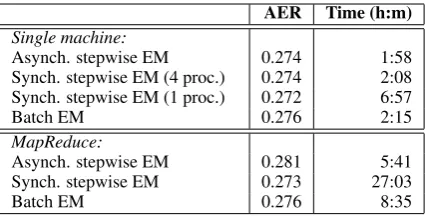
AER Time (h:m)

Single machine:

Asynch. stepwise EM 0.274 1:58

Synch. stepwise EM (4 proc.) 0.274 2:08 Synch. stepwise EM (1 proc.) 0.272 6:57

Batch EM 0.276 2:15

MapReduce:

Asynch. stepwise EM 0.281 5:41

Synch. stepwise EM 0.273 27:03

Batch EM 0.276 8:35

Table 2: Alignment error rates and wall time after 20 itera-tions of EM for various settings. See text for details.

a large MapReduce cluster, but the overhead re-quired for each MapReduce job was too large to make this viable (30–60 seconds).

6.2 Word Alignment

We trained IBM Model 1 in both directions. To align test data, we symmetrized both directional Viterbi alignments using the “grow-diag-final” heuristic (Koehn et al., 2003). We evaluated our models using alignment error rate (AER).

Experiments on a Single Machine We fol-lowed Liang and Klein (2009) in using syn-chronous (mini-batch) stepwise EM on a single processor for this task. We used the same learning rate formula (η(t)= (t+ 2)−q, with0.5< q≤1). We also used asynchronous stepwise EM by using the same update rule, but gathered sufficient statis-tics on 4 processors of a single machine in paral-lel, analogous to our asynchronous method from §5. Whenever a processor was done gathering the expected counts for its mini-batch, it updated the sufficient statistics vector and began work on the next mini-batch.

We used the sparse update described by Liang and Klein, which allows each thread to make additive updates to the parameter vector and to separately-maintained normalization constants without needing to renormalize after each update. When probabilities are needed during inference, normalizers are divided out on-the-fly as needed.

We made 10 passes of asynchronous stepwise EM to measure its sensitivity to q and the mini-batch size m, using different values of these hyperparameters (q ∈ {0.5,0.7,1.0}; m ∈ {5000,10000,50000}), and selected values that maximized log-likelihood (q= 0.7,m= 10000).

Experiments on MapReduce We implemented the three techniques in a MapReduce framework. We implemented batch EM on MapReduce by

converting each EM iteration into two MapRe-duce jobs: one for the E-step and one for the M-step.6 For the E-step, we divided our data into 24 map tasks, and computed expected counts for the source-target parameters at each mapper. Next, we summed up the expected counts in one reduce task. For the M-step, we took the output from the E-step, and in one reduce task, normalized each source-target parameter by the total count for the source word.7 _{To gather sufficient statistics} for synchronous stepwise EM, we used 6 mappers and one reducer for a mini-batch of size 10000. For the asynchronous version, we ran four parallel asynchronous mini-batches, the sufficient statis-tics being gathered using MapReduce again for each mini-batch with 6 map tasks and one reducer.

Results Figure 4 shows log-likelihood for the English→French direction during the first 80 min-utes of optimization. Similar trends were observed for the French→English direction as well as for convergence in AER. Table 2 shows the AER at the end of 20 iterations of EM for the same set-tings.8 It takes around two hours to finish 20 iter-ations of batch EM on a single machine, while it takes more than 8 hours to do so on MapReduce. This is because of the extra overhead of transfer-ringθfrom a master gateway machine to mappers, from mappers to reducers, and from reducers back to the master. Synchronous and asynchronous EM suffer as well.

From Figure 4, we see that synchronous and asynchronous stepwise EM converge at the same rate when each is given 4 processors. The main difference between this task and NER is the size of the mini-batch used, so we experimented with several values for the mini-batch size m. Fig-ure 5 shows the results. Asmdecreases, a larger fraction of time is spent updating parameters; this slows observed convergence time even when us-ing the sparse update rule. It can be seen that, though synchronous and asynchronous stepwise EM converge at the same rate with a large mini-batch size (m = 10000), asynchronous stepwise

6_{The M-step could have been performed without} MapRe-duce by storing all the parameters in memory, but memory restrictions on the gateway node of our cluster prevented this. 7_{For the reducer in the M-step, the source served as the} key, and the target appended by the parameter’s expected count served as the value.

10 20 30 40 50 60 70 80 −40

−35 −30 −25 −20

Log−Likelihood

Asynch. Stepwise EM (4 processors) Synch. Stepwise EM (4 processors) Synch. Stepwise EM (1 processor) Batch EM (1 processor)

10 20 30 40 50 60 70 80

−40 −35 −30 −25 −20

Wall clock time (minutes)

Log−Likelihood

Asynch. Stepwise EM (MapReduce) Synch. Stepwise EM (MapReduce) Batch EM (MapReduce)

Figure 4: English→French log-likelihood vs. wall clock time in minutes on both a single machine (top) and on a large MapReduce cluster (bottom), shown on separate plots for clarity, though axis scales are identical. We show runs of each setting for the first 80 minutes, although EM was run for 20 passes through the data in all cases (Table 2). Fastest convergence is obtained by synchronous and asynchronous stepwise EM using 4 processors on a single node. While the algorithms converge more slowly on MapReduce due to over-head, the asynchronous algorithm converges the fastest. We observed similar trends for the French→English direction.

EM converges faster asm decreases. With large mini-batches, load-balancing becomes less impor-tant as there will be less variation in per-mini-batch observed runtime. These results suggest that asynchronous mini-batch algorithms will be most useful for learning problems in which small mini-batches work best. Fortunately, however, we do not see any problems stemming from approxima-tion errors due to the use of asynchronous updates.

6.3 Unsupervised POS Tagging

Our unsupervised POS experiments use the same task and approach of Liang and Klein (2009) and so we fix hyperparameters for stepwise EM based on their findings (learning rateη(t) = (t+ 2)−0.7). The asynchronous algorithm uses the same learn-ing rate formula as the slearn-ingle-processor algorithm. There is only a singletthat is maintained and gets incremented whenever any thread updates the pa-rameters. Liang and Klein used a mini-batch size of 3, but we instead use a mini-batch size of 4 to better suit our 4-processor synchronous and asyn-chronous architectures.

Like NER, we present results for unsupervised tagging experiments on a single machine only, i.e., not using a MapReduce cluster. For tasks like POS tagging that have been shown to work best with small mini-batches (Liang and Klein, 2009), we

10 20 30 40 50 60 70 80

−35 −30 −25 −20

Wall clock time (minutes)

Log−Likelihood

Asynch. (m = 10,000) Synch. (m = 10,000) Asynch. (m = 1,000) Synch. (m = 1,000) Asynch. (m = 100) Synch. (m = 100)

Figure 5: English→French log-likelihood vs. wall clock time in minutes for stepwise EM with 4 processors for various mini-batch sizes (m). The benefits of asynchronous updat-ing increase asmdecreases.

did not conduct experiments with MapReduce due to high overhead per mini-batch.

For initialization, we followed Liang and Klein by initializing each parameter as θi ∝ e1+ai, ai ∼ Uniform([0,1]). We generated 5 random

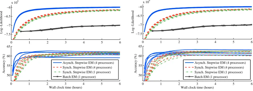
models using this procedure and used each to ini-tialize each algorithm. We additionally used 2 random seeds for choosing the ordering of exam-ples,9 resulting in a total of 10 runs for each al-gorithm. We ran each for six hours, saving mod-els every five minutes. After training completed, using each model we decoded the entire training data using posterior decoding and computed the log-likelihood. The results for 5 initial models and two example orderings are shown in Figure 6. We evaluated tagging performance using many-to-1 accuracy, which is obtained by mapping the HMM states to gold standard POS tags so as to maximize accuracy, where multiple states can be mapped to the same tag. This is the metric used by Liang and Klein (2009) and Johnson (2007), who report fig-ures comparable to ours. The asynchronous algo-rithm converges much faster than the single-node algorithm, allowing a tagger to be trained from the Penn Treebank in less than two hours using a single machine. Furthermore, the 4-processor synchronous algorithm improves only marginally

9

0 1 2 3 4 5 6 −7.5

−7 −6.5 −6

x 106

Log−Likelihood

0 1 2 3 4 5 6

50 55 60 65

Wall clock time (hours)

Accuracy (%)

Asynch. Stepwise EM (4 processors) Synch. Stepwise EM (4 processors) Synch. Stepwise EM (1 processor) Batch EM (1 processor)

0 1 2 3 4 5 6

−7.5 −7 −6.5 −6

x 106

Log−Likelihood

0 1 2 3 4 5 6

50 55 60 65

Wall clock time (hours)

Accuracy (%)

Asynch. Stepwise EM (4 processors) Synch. Stepwise EM (4 processors) Synch. Stepwise EM (1 processor) Batch EM (1 processor)

Figure 6: POS: Asynchronous stepwise EM converges faster in log-likelihood and accuracy than the synchronous versions. Curves are shown for each of 5 random initial models. One example ordering random seed is shown on the left, another on the right. The accuracy curves for batch EM do not appear because the highest accuracy reached is only 40.7% after six hours.

over the 1-processor baseline.

The accuracy of the asynchronous curves of-ten decreases slightly after peaking. We can sur-mise from the log-likelihood plot that the drop in accuracy is not due to the optimization be-ing led astray, but probably rather due to the complex relationship between likelihood and task-specific evaluation metrics in unsupervised learn-ing (Merialdo, 1994). In fact, when we exam-ined the results of synchronous stepwise EM be-tween 6 and 12 hours of execution, we found sim-ilar drops in accuracy as likelihood continued to improve. From Figure 6, we conclude that the asynchronous algorithm has no harmful effect on learned model’s accuracy beyond the choice to op-timize log-likelihood.

While there are currently no theoretical conver-gence results for asynchronous optimization algo-rithms for non-convex functions, our results are encouraging for the prospects of establishing con-vergence results for this setting.

7 Discussion

Our best results were obtained by exploiting mul-tiple processors on a single machine, while exper-iments using a MapReduce cluster were plagued by communication and framework overhead.

Since Moore’s Law predicts a continual in-crease in the number of cores available on a sin-gle machine but not necessarily an increase in the speed of those cores, we believe that algorithms that can effectively exploit multiple processors on a single machine will be increasingly useful. Even today, applications in NLP involving rich-feature structured prediction, such as parsing and

transla-tion, typically use a large portion of memory for storing pre-computed data structures, such as lex-icons, feature name mappings, and feature caches. Frequently these are large enough to prevent the multiple cores on a single machine from being used for multiple experiments, leaving some pro-cessors unused. However, using multiple threads in a single program allows these large data struc-tures to be shared and allows the threads to make use of the additional processors.

We found the overhead incurred by the MapRe-duce programming model, as implemented in Hadoop 0.20, to be substantial. Nonetheless, we found that asynchronously running multiple MapReduce calls at the same time, rather than pooling all processors into a single MapReduce call, improves observed convergence with negli-gible effects on performance.

8 Conclusion

We have presented experiments using an asyn-chronous framework for distributed mini-batch optimization that show comparable performance of trained models in significantly less time than traditional techniques. Such algorithms keep pro-cessors in constant use and relieve the programmer from having to implement load-balancing schemes for each new problem encountered. We expect asynchronous learning algorithms to be broadly applicable to training NLP models.

References

P. F. Brown, V. J. Della Pietra, S. A. Della Pietra, and R. L. Mercer. 1993. The mathematics of statistical machine translation: parameter estimation.

Compu-tational Linguistics, 19(2):263–311.

O. Capp´e and E. Moulines. 2009. Online EM algo-rithm for latent data models. Journal of the Royal Statistics Society: Series B (Statistical Methodol-ogy), 71.

D. Chiang, Y. Marton, and P. Resnik. 2008. On-line large-margin training of syntactic and structural translation features. InProc. of EMNLP.

C. Chu, S. Kim, Y. Lin, Y. Yu, G. Bradski, A. Ng, and K. Olukotun. 2006. Map-Reduce for machine learn-ing on multicore. InNIPS.

S. Clark and J.R. Curran. 2004. Log-linear models for wide-coverage CCG parsing. InProc. of EMNLP. M. Collins. 2002. Ranking algorithms for

named-entity extraction: Boosting and the voted perceptron.

InProc. of ACL.

K. Crammer and Y. Singer. 2003. Ultraconservative online algorithms for multiclass problems. Journal

of Machine Learning Research, 3:951–991.

K. Crammer, O. Dekel, J. Keshet, S. Shalev-Shwartz, and Y. Singer. 2006. Online passive-aggressive al-gorithms. Journal of Machine Learning Research, 7:551–585.

J. Dean and S. Ghemawat. 2004. MapReduce: Sim-plified data processing on large clusters. In Sixth Symposium on Operating System Design and

Imple-mentation.

C. Dyer, A. Cordova, A. Mont, and J. Lin. 2008. Fast, easy, and cheap: Construction of statistical machine translation models with MapReduce. InProc. of the

Third Workshop on Statistical Machine Translation.

J. R. Finkel, A. Kleeman, and C. D. Manning. 2008. Efficient, feature-based, conditional random field parsing. InProc. of ACL.

M. Johnson. 2007. Why doesn’t EM find good HMM POS-taggers? InProc. of EMNLP-CoNLL.

J. Kazama and K. Torisawa. 2007. A new perceptron algorithm for sequence labeling with non-local fea-tures. InProc. of EMNLP-CoNLL.

P. Koehn, F. J. Och, and D. Marcu. 2003. Statistical phrase-based translation. InProc. of HLT-NAACL. J. Lafferty, A. McCallum, and F. Pereira. 2001.

Con-ditional random fields: Probabilistic models for seg-menting and labeling sequence data. In Proc. of

ICML.

J. Langford, A. J. Smola, and M. Zinkevich. 2009. Slow learners are fast. InNIPS.

Y. LeCun, L. Bottou, Y. Bengio, and P. Haffner. 1998. Gradient-based learning applied to document recog-nition.Proceedings of the IEEE, 86(11):2278–2324. P. Liang and D. Klein. 2009. Online EM for

unsuper-vised models. InProc. of NAACL-HLT.

G. Mann, R. McDonald, M. Mohri, N. Silberman, and D. Walker. 2009. Efficient large-scale distributed training of conditional maximum entropy models. InNIPS.

M. P. Marcus, B. Santorini, and M. A. Marcinkiewicz. 1993. Building a large annotated corpus of En-glish: The Penn treebank. Computational Linguis-tics, 19:313–330.

B. Merialdo. 1994. Tagging English text with a probabilistic model. Computational Linguistics, 20(2):155–172.

R. Mihalcea and T. Pedersen. 2003. An evaluation exercise for word alignment. InHLT-NAACL 2003 Workshop: Building and Using Parallel Texts: Data

Driven Machine Translation and Beyond.

R. Neal and G. E. Hinton. 1998. A view of the EM al-gorithm that justifies incremental, sparse, and other variants. InLearning in Graphical Models.

A. Nedic, D. P. Bertsekas, and V. S. Borkar. 2001. Distributed asynchronous incremental subgradient methods. InProc. of the March 2000 Haifa Work-shop: Inherently Parallel Algorithms in Feasibility

and Optimization and Their Applications.

N. Ratliff, J. Bagnell, and M. Zinkevich. 2006. Sub-gradient methods for maximum margin structured learning. InICML Workshop on Learning in

Struc-tured Outputs Spaces.

M. Sato and S. Ishii. 2000. On-line EM algorithm for the normalized Gaussian network. Neural

Compu-tation, 12(2).

B. Taskar, V. Chatalbashev, D. Koller, and C. Guestrin. 2005. Learning structured prediction models: A large margin approach. InProc. of ICML.

E. F. Tjong Kim Sang and F. De Meulder. 2003. Intro-duction to the CoNLL-2003 shared task: Language-independent named entity recognition. InProc. of

CoNLL.

I. Tsochantaridis, T. Joachims, T. Hofmann, and Y. Al-tun. 2005. Large margin methods for structured and interdependent output variables. Journal of Machine

Learning Research, 6:1453–1484.

J. Wolfe, A. Haghighi, and D. Klein. 2008. Fully distributed EM for very large datasets. In Proc. of