e-ISSN: 2278-067X, p-ISSN: 2278-800X, www.ijerd.com
Volume 13, Issue 12 (December 2017), PP.01-11
1
Optimized Support Vector Machine for Software Defect
Prediction
1
M. Thangavel,
2Dr. R. Pugazendi
1Department of Computer Science, Government Arts College(Autonomous),Salem-7. 2
Department of Computer Science, Government Arts College(Autonomous),Salem-7. Corresponding Author: M.Thangavel
ABSTRACT
: An error, bug, flaw, failure, mistake or fault in a computer program or system that generates inaccurate/unexpected outcome or prevents software from behaving as intended is a software defect. A project team wants to procreate a quality software product with zero defects. High-risk components in a software project must be caught early to enhance software quality. Software defects incur cost regarding quality and time. This article investigates Support Vector Machine’s (SVM) classification accuracy for Software Defect Prediction (SDP) and proposes a new optimized MRMR and SVM with firefly algorithm.Keywords:- Software Defect, Software Defect Prediction (SDP), optimized Support Vector Machine Radial Basis Function (SVM – RBF), Firefly.
Date of Submission: 20 -11-2017 Date of acceptance: 28-12-2017
I.
INTRODUCTION
Defects can be defined in disparate ways but are generally aberration from specifications or ardent expectations which lead to procedure failures. Defect data analysis of classification and prediction types to extract models describing significant defect data classes or predict future defect trends. Classification predicts categorical/discrete, and unordered labels, while prediction models predict continuous valued functions. Such analysis provides better understanding of software defect data [1].
Software Defect Prediction (SDP) is essential in software engineering. Predicting defect is a proactive process, characterizing defect types in software’s content, design and codes to produce a high-quality product. Predicting defects in a system testing phase especially functional defects are important in test process improvement [2]. Software teams tries to produce a zero defect product. Defect prediction leads to a high-quality product and high-quality assurance. Software defects prediction reduces software testing efforts by guiding testers through software systems defect classification. If a defective product goes to customers it leads to issues. A defect reduces software reliability. Predicting defects needs practice and knowledge. Hence, defect prediction is important in software quality and software reliability [3].
Feature selection is a data preprocessing activity extensively studied in the machine learning and data mining community. The goal of feature selection is selecting a features subset that reduces classifiers prediction errors [4]. Feature selection techniques are divided into wrapper-based approaches and filter-based approaches. The former involves training a learner during feature selection, while the latter uses data intrinsic characteristics for feature selection based on a metric without depending on training a learner. The advantage of a filter-based approach over a wrapper-based approach is its faster computation. But, if computational complexity is not a factor, then a wrapper-based approach is the best overall feature selection scheme regarding accuracy [5].
Classification finds a set of models that describe/distinguish data classes/concepts. The derived model is represented in forms like classification rules and decision trees. When classes are defined the system infers rules governing classification. Hence, a system should find a description of each class. A description should refer to the training set’s prediction attributes so that positive examples satisfy the description. A rule is correct if its description covers all positive examples of a class [6].
software defect prediction. Experiments were conducted on data sets and results were compared with other classifiers. Satisfactory performance without losing comprehensibility resulted.
SDP is a supervised binary classification problem. Software modules are represented by software metrics being labeled defective or non-defective. To learn defect predictors, data tables of historical examples are formed; one column has a Boolean value for ‖defects detected‖ (dependent variable) and other columns describe software characteristics regarding software metrics (independent variables) [9].
Naive Bayesian classifier is a Bayes theorem based with independence assumptions between predictors. The model is easy to build, having no complicated iterative parameter estimation making it useful for large datasets. Despite simplicity, a Naive Bayesian classifier does surprisingly well and is used as it outperforms other sophisticated classification methods [7].
Classification divides data samples into target classes. Software modules are categorized as ―defective‖ or ―not-defective‖ by classification approaches. In Classification, class categories are known and so it is a supervised learning approach [10]. There are two classification methods: Binary and Multilevel. Binary classification divides a class into 2 categories; ―defective‖ and ―not-defective‖. While Multi-level classification is used when there are more than two classes. It divides a class as ―highly complex‖, ―complex‖ or ―simple‖ software programs. Classification approach works in Learning and Testing phases. So, it divides a dataset into training and testing parts. Various approaches like cross fold, Leave-one-out partition a dataset. During learning phase, a classifier learns using a training dataset and is evaluated using a testing dataset[11].
SVM formulation was proposed by Vapnik et al., in 1990s based on statistical learning theory [12]. SVM was developed to solve 2 classification problems but was later formulated and extended to solve multiclass problem [13]. SVM divides data samples of both classes by determining a hyper-plane in original input space maximizing the separation between them. SVM works effectively for data samples classification not separable linearly, by using the kernel function theory. Many kernel functions for example Gaussian, Polynomial and Sigmoid are available to map data samples into higher dimension feature space. SVM determines a hyper-plane in feature space to divide data samples of different classes [14]. Thus, it is a better choice for both linearly and nonlinearly separable data classification.
SVM has many advantages like providing a global data classification solution. It generates a unique global hyper-plane to separate different classes data samples rather than local boundaries as compared with other current data classification approaches. As SVM follows a Structural Risk Minimization (SRM) principle, it reduces risk occurrence during training phase and also enhances generalization capability [15]. A data sample on and near hyper-plane is termed support vector. SVM is used by researchers to construct a predictive SDP model [16]. This article investigates SVM’s classification accuracy for SDP. It proposes MRMR and SVM with firefly algorithm.
II.
LITERATURE REVIEW
A work to validate predictor feasibility built with a simplified metric set for SDP in different scenarios was presented by He et al., [17]. It investigated practical guidelines for training data choice, classifier and metric subset of a project. First, based on 6 classifiers, it constructed 3 types of predictors using the software metric set size in 3 scenarios. Next, it validated the predictor’s acceptable performance based on Top-k metrics regarding statistical methods. Finally, it tried to minimize a Top-k metric subset by removing redundant metrics. Its stability was tested by a one-way ANOVA tests.
A new dynamic SVM method based on improved cost-sensitive SVM (CSSVM) optimized by a GA was proposed by Shuai et al., [18]. The GA through selecting geometric classification accuracy as fitness function improved the performance of CSSVM by enhancing the defective modules accuracy and reducing total cost of the whole decision. Results showed that GA-CSSVM achieved higher AUC value denoting better prediction accuracy for minority and majority samples in an imbalanced software defect data set.
3
A new model for SDP using PSO and SVM called P-SVM model proposed by Can et al., [20] takes advantage of SVM’s non-linear computing capability and PSO’s parameters optimization capability. P-SVM uses PSO algorithm to calculate SVM’s best parameters and adopts the optimized SVM model to predict software defect. Results showed that P-SVM had a higher prediction accuracy than BP NN, SVM, and GA-SVM.
A novel model based on Locally Linear Embedding and SVM (LLE-SVM) was proposed by Shan et al., [21]. SDP improves software security by helping testers locate software defects accurately. SVM is used as basic classifier in the model and LLE algorithm solves data redundancy by its ability to maintain local geometry. A comparison between LLE-SVM and SVM was experimentally verified on the NASA defect data set. Results indicate that new LLE-SVM model performs better than SVM model, and it avoids accuracy decrease due data redundancy.
A static code metrics for a collection of modules in eleven NASA data sets used with a SVM classifier was presented by Gray et al., [22]. Rigorous pre-processing steps were applied to data prior to classification, including balancing both classes (defective or otherwise) and removal of many repeating instances. The SVM in this experiment yielded an average of 70% accuracy on previously unseen data.
A hybrid attribute selection approach, where feature ranking is used to reduce search space, followed by feature subset selection was proposed by Gao et al., [23]. Seven different feature ranking techniques were evaluated, and 4 different feature subset selection approaches considered. The models are trained with 5 common classification algorithms. The study is based on software metrics and defective data from multiple releases of a large real-world software system. Results proved that while some feature ranking techniques performed the same, automatic hybrid search algorithm performed the best among feature subset selection methods.
A new method of using Fuzzy Support Vector Regression (FSVR) to predict software defect numbers was proposed by Yan et al., [24] . Fuzzification regressor input handles unbalanced software metrics dataset. Compared to support vector regression approach, the experiment conducted by applying MIS and RSDIMU datasets inferred that FSVR leads to lower mean squared error and higher total defects accuracy for modules with large number of defects.
A rough hybrid approach was compared with neuro-fuzzy and partial decision trees to classify software defect data by Bhatt et al., [25]. The extension has a comparison with linear and non-linear SVMs to classify defects. It also compared SVM classification results with neuro-fuzzy decision trees (NFDT), partial decision trees, and LEM2 algorithm based on rough sets, fuzzy-rough classification trees (FRCT) and rough-neuro-fuzzy decision trees (R-NFDT). The result analyses included statistical tests for classification accuracy.
A comprehensive empirical study examining 17 different ensembles of feature ranking techniques (rankers) including 6 common feature ranking techniques, signal-to-noise filter technique and 11 threshold-based feature ranking techniques was presented by Wang et al., [26]. This study used 16 real-world software measurement data sets of various sizes and built 13,600 classification models. Results indicated that ensembles of few rankers are effective and better than those of many or all rankers.
III.
METHODOLOGY
Dataset
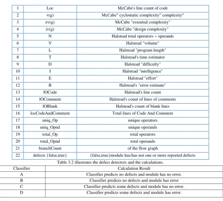
Table 3.1. LIST OF KC1 DATASET ATTRIBUTES
1 Loc McCabe's line count of code
2 v(g) McCabe" cyclomatic complexity‖ complexity"
3 ev(g) McCabe "essential complexity"
4 iv(g) McCabe "design complexity"
5 N Halstead total operators + operands
6 V Halstead "volume"
7 L Halstead "program length"
8 T Halstead's time estimator
9 D Halstead "difficulty"
10 I Halstead "intelligence"
11 E Halstead "effort"
12 B Halstead's "error estimate"
13 lOCode Halstead's line count
14 lOComment Halstead's count of lines of comments
15 lOBlank Halstead's count of blank lines
16 locCodeAndComment Total lines of Code And Comment
17 uniq_Op unique operators
18 uniq_Opnd unique operands
19 total_Op total operators
20 total_Opnd total operands
21 branchCount of the flow graph
22 defects {false,true} {false,true}module has/has not one or more reported defects Table 3.2 illustrates the defect detectors and the calculations.
Classifier Calculation Result
A Classifier predicts no defects and module has no error.
B Classifier predicts no defects and module has error
C Classifier predicts some defects and module has no error.
D Classifier predicts some defects and module has error.
Detection probability (pd) or recall, precision (prec), Accuracy, probability of false alarm (pf), and effort are calculated using the formulas.
a d A c c u r a c y
a b c d
(1)
d r e c a ll
b d
(2)
c p f
a c
(3)
d p r e c
c d
(4)
. .
c L O C d L O C e ffo r t
T o ta lL O C
(5)
5
Feature selection - Minimum Redundancy — Maximum Relevance (MRMR)
Feature Selection (FS), also called attribute selection, is a significant issue in classification model construction. Feature selection reduces input features and selects relevant features for a classifier to improve predictive performance. FS obtains relevant data for future analysis, as per problem formulation. As there are many software metrics available in the software dataset repository, so FS selects significant features which reduces total project cost [28].When a feature has expressions randomly/uniformly distributed in different classes, its mutual information with such classes is zero. If a feature is differentially expressed for different classes, it has large mutual information. So, mutual information is a measure of features relevance. For discrete/categorical variables, mutual information I of two variables x and Y is defined based on the joint probabilistic distribution P(x,Y) and respective marginal probabilities p(x) and p(y):
,,
, i, i lo g i i
i j i i
p x y I x y p x y
p x p y
. (6)For categorical variables, mutual information measures level of "similarity" between features. The idea of minimum redundancy is selecting features so that they are mutually maximally dissimilar. Minimal redundancy makes feature sets a better representation of the dataset. Let S denote a subset of features sought. Minimum redundancy condition is
2 , 1
m in I, I ,
i j S
W W I i j
S
, (7)where I (i, j) represents I (gi , gj) for notational simplicity, and (= m) is number of features in S.
To measure level of discriminant powers of genes when differentially expressed for different target classes, mutual information I (h, gi) between targeted classes h = {hl, h2,..., hK } (h classification variable) is used and feature expression gi.
I (h, gi) quantifies relevance of gi for classification task. Thus, maximum relevance condition is maximizing total relevance of all genes in S:
1
m a x I, I ,
i S
V V I h i S
where I (h, gi) is referred as I (h, i) (8)Minimum Redundancy — Maximum Relevance (MRMR) feature set is got by optimizing the conditions in the above equations simultaneously. Optimization of both conditions combines them into a single criterion function. This paper treats both conditions as equally important and considers two simple combination criteria:
m a x VI WI , m a x
VI WI
. (9)For continuous data variables (or attributes), the F -statistic between features and classification variable h as score of maximum relevance is chosen. The F -test value of feature variable gi in K classes denoted by h has the following form
2, 1
i k k
k
F g h n g g K
, (10)
where g- is mean value of gi in samples, g-k is mean value of gi within the kth class, and
2
1
k
k
n n k
(11)
is pooled variance (where nk and σk are the size and variance of kth class). F- test reduces to t-test for 2-class classification,
with the relation F = t2. Hence, for feature set S, maximum relevance is written as:
1
m a x F, F ,
i S
V V F i h S
IV.
SUPPORT VECTOR MACHINE (SVM)
SVM classifier is trained before use; thus reduced input data is partitioned (yi), i=l,…,n into 2, T
⊂{l,…,n} training set and V ⊂{l,…,n} testing (or validation) set with T ∪ V = {l,…,n} and T ∩V={}. Training data set T is labeled manually into 2 classes with ground truth, l(yi)=±1. Once classifier is trained and decision function evaluation d(yi)= ±1 yields classification of any data yi. In detail, SVM [11] tries to separate data φ(yi) mapped by selected kernel function φ by a hyperplane wTφ(yi)+b=0 with w normal vector and b translation. Decision function is d(yi) =sgn(wTφ(yi)+b). Maximizing margin and introducing slack variables ζ = (ζ i) for non-separable data, a primal optimization problem is received:
, , 1 m i n
2 1 0 , T i w b i T T
i i i
i
w w C
w i t h c o n s t r a i n s l y w y b f o r i T
(13)where C is user-determined penalty parameter. Easier computation is possible when switched to dual optimization problem,
1 m i n
2 0 0 , T T i i i i T Q e
w i t h c o n s t r a i n s C f o r i T y
where α = (αi) are so-called support vectors, e = [l,…,l]T and Q is positive semi-definite matrix formed by Qjk= /(yj)/(yk)K(yj,yk), and K(yj,yk) =φ(yj)T φ(yk) is kernel function from φ. When optimization problem is solved,
hyperplane parameters w and b, w are determined directly as i
i ii T
w l y y
and b via one ofKarush-Kuhn-Tucker conditions as b = -l(yi)yiTw, for those i with 0<αi C. So, trained SVM classifier's decision function ends up as
i s g n
T
i
s g n j
j j, i
j T
d y w y b l y K y y b
(14)Inner feature space product has equal kernel in input space [29],
, '
, 'K x x x x
When certain conditions hold. When K is a symmetric positive definite function that satisfies Mercer's Conditions
2, ' ' 0 ,
, ' ' ' 0 , g L ,
m m m m
m
K x x a x x a
K x x g x g x d x d x
(15)7
Radial basis functions (RBF) received attention, usually with a Gaussian of form,
2 2
' , ' e x p
2
x x K x x
. (16)
Classical techniques with RBF are centers subset determiners. Clustering selects a centers subset first. SVM feature' attraction is that selection with support vectors contributes one local Gaussian function centered on data point which is implicit.
Parameter selection is crucial as SVM algorithm is sensitive to adequate parameter values choice and affects prediction accuracy. In SVM, parameters regularization constant C, and coefficients of SV kernel, e.g. kernel width σ in RBF impact prediction. Regularization parameter C determines trade-off cost between minimizing training error and minimizing model complexity, which reduces generalization capability when set too small or excessive. And σ reflects support vector correlation which determines generalization capability and prediction accuracy. Selecting cost parameter is NP hard. This work proposes using a new Firefly algorithm to locate the ideal C parameter.
Firefly algorithm is based on fireflies flashing lights. In a firefly algorithm, the objective function of an optimization problem is associated with flashing light or light intensity which helps a firefly swarm to move to brighter/more attractive locations to get efficient optimal solutions. Some flashing characteristics of fireflies are idealized to develop a firefly-inspired algorithm [30].
The following 3 idealized rules were used to describe the new Fireflies Algorithm,: 1) all fireflies are unisex so one firefly is attracted to another regardless of sex; 2) Attractiveness is proportional to brightness, so for 2 flashing fireflies, the less brighter moves toward the brighter one. As attractiveness is proportional to brightness it decreases as distance increases. If there is no brighter firefly it moves randomly; 3) a firefly’s brightness is affected/determined by the objective function’s landscape.
For a maximization problem, the brightness is proportional to the objective function value. Other forms of brightness are defined similar to a fitness function in Gas. The basic steps of a FA are as follows based on the above rules:
3. 4.
Objective function f(x), x = (x
1,..., x
d)T
Generate initial population of fireflies x
i(i = 1, 2,..., n)
Light intensity I
iat x
iis determined by f(x
i)
Define light absorption coefficient γ
while (t <MaxGeneration)
for i = 1 : n all n fireflies
for j = 1 : i all n fireflies
if (I
j> I
i), Move firefly i towards j in d-dimension; end if
Attractiveness varies with distance r via exp[−γr]
Evaluate new solutions and update light intensity
end for j
end for i
Rank the fireflies and find the current best
end while
V.
RESULTS AND DISCUSSION
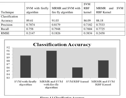
The software complexity measures such as Cyclomatic complexity, Base Halstead measures, Derived Halstead measures, and LOC measure of KC1 (NASA) dataset are used to classify the software modules. All classification in this investigation is carried out on Weka. For the performance evaluation of classifiers, 2107 samples from KC1 Dataset is used, where 716 samples are used as testing set, and 1391samples are used for training. Weka was used on KC1 dataset for classification, and result is summarized in Table 4.1 and Figure 4.1.
Table 4.1 Results
Technique
SVM with firefly algorithm
MRMR and SVM with fire fly algorithm
SVM RBF kernel
MRMR and SVM RBF Kernel
Classification
Accuracy 89.61 91.03 86.09 88.18
Precision 0.7874 0.8179 0.7182 0.7533
Recall 0.758 0.7948 0.7604 0.7725
RMSE 0.2147 0.1826 0.3834 0.2458
Figure4.1 Classification Accuracy
The MRMR and SVM with firefly algorithm improved the classification accuracy by 5.58% when compared to the SVM.
Figure 4.2 Precision
9
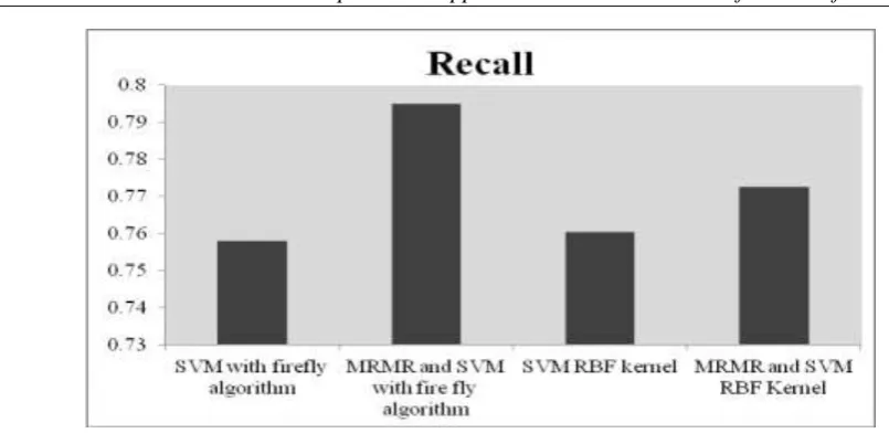
Figure 4.3 Recall
The MRMR and SVM with firefly algorithm improved recall by 1.91% when compared to the SVM with firefly algorithm.
Figure 4.4 RMSE
The MRMR and SVM with firefly algorithm reduced RMSE by 13.5071% when compared to the SVM with firefly algorithm.
V CONCLUSION
Software defects are expensive regarding quality and cost. Also, the cost of capturing and correcting defects is a very expensive software development activity. SVM is popular and most of the researchers use it to construct a predictive model for SDP. Parameter selection is crucial as SVM algorithm is sensitive to the choice of parameter values affecting prediction accuracy. This article proposes a new optimized MRMR and SVM with firefly algorithm (MRMR-SVM with firefly algorithm) to predict SDP. Experiments show that the new method improved classification accuracy.
REFERENCES
[1]. Rawat, M. S., & Dubey, S. K. (2012). Software defect prediction models for quality improvement: a literature study. International Journal of Computer Science.
[2]. Clark, B., & Zubrow, D. (2001). How good is the software: a review of defect prediction techniques. sponsored by the US department of Defense.
[4]. Wahono, R. S., & Suryana, N. (2013). Combining Particle Swarm Optimization based Feature Selection and Bagging Technique for Software Defect Prediction.International Journal of Software Engineering & Its Applications, 7(5).
[5]. Menzies, T., Milton, Z., Turhan, B., Cukic, B., Jiang, Y., & Bener, A. (2010). Defect prediction from static code features: current results, limitations, new approaches. Automated Software Engineering, 17(4), 375-407.
[6]. Kaur, M. P. J., & Pallavi, M. (2013). Data mining techniques for software defect prediction. International Journal of Software and Web Sciences, 54-57.
[7]. Baojun, M., Dejaeger, K., Vanthienen, J., & Baesens, B. (2011). Software defect prediction based on association rule classification. Available at SSRN 1785381.
[8]. Liu, B., Ma, Y., & Wong, C. K. (2000). Improving an association rule based classifier. In Principles of Data Mining and Knowledge Discovery (pp. 504-509). Springer Berlin Heidelberg.
[9]. Song, Q., Jia, Z., Shepperd, M., Ying, S., & Liu, J. (2011). A general software defect-proneness prediction framework. Software Engineering, IEEE Transactions on, 37(3), 356-370.
[10]. Jiawei, H., & Kamber, M. (2001). Data mining: concepts and techniques. San Francisco, CA, itd: Morgan Kaufmann, 5.
[11]. Agarwal, S., & Tomar, D. (2014). A Feature Selection Based Model for Software Defect Prediction. assessment, 65.
[12]. Cortes, C., & Vapnik, V. (1995). Support-vector networks. Machine learning,20(3), 273-297.
[13]. Dietterich, T. G., & Bakiri, G. (1995). Solving multiclass learning problems via error-correcting output codes. arXiv preprint cs/9501101.
[14]. Schölkopf, B., Burges, C. J., & Smola, A. J. (Eds.). (1999). Advances in kernel methods: support vector learning. MIT press.
[15]. Sastry, P. S. (2003). An introduction to support vector machines. Computing and information sciences: Recent trends, 53-85.
[16]. Sundararaghavan, V., & Zabaras, N. (2005). Classification and reconstruction of three-dimensional microstructures using support vector machines.Computational Materials Science, 32(2), 223-239. [17]. He, P., Li, B., Liu, X., Chen, J., & Ma, Y. (2014). An Empirical Study on Software Defect Prediction
with Simplified Metric Set. arXiv preprint arXiv:1402.3873.
[18]. Shuai, B., Li, H., Li, M., Zhang, Q., & Tang, C. (2013, December). Software Defect Prediction Using Dynamic Support Vector Machine. In Computational Intelligence and Security (CIS), 2013 9th International Conference on (pp. 260-263). IEEE.
[19]. Agarwal, S., & Tomar, D. (2014, March). Prediction of software defects using Twin Support Vector Machine. In Information Systems and Computer Networks (ISCON), 2014 International Conference on (pp. 128-132). IEEE.
[20]. Can, H., Jianchun, X., Ruide, Z., Juelong, L., Qiliang, Y., & Liqiang, X. (2013, May). A new model for software defect prediction using particle swarm optimization and support vector machine. In Control and Decision Conference (CCDC), 2013 25th Chinese (pp. 4106-4110). IEEE.
[21]. Shan, C., Chen, B., Hu, C., Xue, J., & Li, N. (2014, May). Software defect prediction model based on LLE and SVM. In Communications Security Conference (CSC 2014), 2014 (pp. 1-5). IET.
[22]. Gray, D., Bowes, D., Davey, N., Sun, Y., & Christianson, B. (2009). Using the support vector machine as a classification method for software defect prediction with static code metrics. In Engineering Applications of Neural Networks (pp. 223-234). Springer Berlin Heidelberg.
[23]. Gao, K., Khoshgoftaar, T. M., Wang, H., & Seliya, N. (2011). Choosing software metrics for defect prediction: an investigation on feature selection techniques. Software: Practice and Experience, 41(5), 579-606.
[24]. Yan, Z., Chen, X., & Guo, P. (2010). Software defect prediction using fuzzy support vector regression. In Advances in Neural Networks-ISNN 2010 (pp. 17-24). Springer Berlin Heidelberg.
11
[26]. Wang, H., Khoshgoftaar, T. M., & Napolitano, A. (2010, December). A comparative study of ensemble feature selection techniques for software defect prediction. In Machine Learning and Applications (ICMLA), 2010 Ninth International Conference on (pp. 135-140). IEEE.
[27]. Shirabad, J. S., & Menzies, T. J. (2005). The PROMISE repository of software engineering databases. School of Information Technology and Engineering, University of Ottawa, Canada, 24. [28]. Akay, M. F. (2009). Support vector machines combined with feature selection for breast cancer
diagnosis. Expert systems with applications, 36(2), 3240-3247.
[29]. Gunn, S. R. (1998). Support vector machines for classification and regression.ISIS technical report, 14. [30]. X.-S. Yang, ―Firefly algorithms for multimodal optimization,‖ in Stochastic Algorithms: Foundations and
Applications(Springer, 2009), pp. 169–178.