c
2004 Hindawi Publishing Corporation
A Digital Synthesis Model of Double-Reed
Wind Instruments
Ph. Guillemain
Laboratoire de M´ecanique et d’Acoustique, Centre National de la Recherche Scientifique, 31 chemin Joseph-Aiguier, 13402 Marseille cedex 20, France
Email:[email protected]
Received 30 June 2003; Revised 29 November 2003
We present a real-time synthesis model for double-reed wind instruments based on a nonlinear physical model. One specificity of double-reed instruments, namely, the presence of a confined air jet in the embouchure, for which a physical model has been proposed recently, is included in the synthesis model. The synthesis procedure involves the use of the physical variables via a digital scheme giving the impedance relationship between pressure and flow in the time domain. Comparisons are made between the behavior of the model with and without the confined air jet in the case of a simple cylindrical bore and that of a more realistic bore, the geometry of which is an approximation of an oboe bore.
Keywords and phrases:double-reed, synthesis, impedance.
1. INTRODUCTION
The simulation of woodwind instrument sounds has been in-vestigated for many years since the pioneer studies by Schu-macher [1] on the clarinet, which did not focus on digital sound synthesis. Real-time-oriented techniques, such as the famous digital waveguide method (see, e.g., Smith [2] and V¨alim¨aki [3]) and wave digital models [4] have been intro-duced in order to obtain efficient digital descriptions of res-onators in terms of incoming and outgoing waves, and used to simulate various wind instruments.
The resonator of a clarinet can be said to be approxi-mately cylindrical as a first approximation, and its embou-chure is large enough to be compatible with simple airflow models. In double-reed instruments, such as the oboe, the resonator is not cylindrical but conical and the size of the air jet is comparable to that of the embouchure. In this case, the dissipation of the air jet is no longer free, and the jet remains confined in the embouchure, giving rise to additional aero-dynamic losses.
Here, we describe a real-time digital synthesis model for double-reed instruments based on one hand on a recent study by Vergez et al. [5], in which the formation of the con-fined air jet in the embouchure is taken into account, and on the other hand on an extension of the method presented in [6] for synthesizing the clarinet. This method avoids the need for the incoming and outgoing wave decompositions, since it deals only with the relationship between the impedance vari-ables, which makes it easy to transpose the physical model to a synthesis model.
The physical model is first summarized inSection 2. In order to obtain the synthesis model, a suitable form of the flow model is then proposed, a dimensionless version is writ-ten and the similarities with single-reed models (see, e.g., [7]) are pointed out. The resonator model is obtained by as-sociating several elementary impedances, and is described in terms of the acoustic pressure and flow.
Section 3presents the digital synthesis model, which re-quires first discrete-time equivalents of the reed displacement and the impedance relations. The explicit scheme solving the nonlinear model, which is similar to that proposed in [6], is then briefly summarized.
InSection 4, the synthesis model is used to investigate the effects of the changes in the nonlinear characteristics induced by the confined air jet.
2. PHYSICAL MODEL
The main physical components of the nonlinear synthesis model are as follows.
(i) The linear oscillator modeling the first mode of reeds vibration.
(ii) The nonlinear characteristics relating the flow to the pressure and to the reed displacement at the mouth-piece.
(iii) The impedance equation linking pressure and flow.
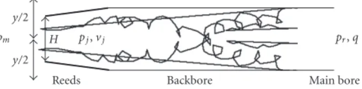
pm y/2
y/2
H pj,vj pr,q
Reeds Backbore Main bore
Figure1: Embouchure model and physical variables.
2.1. Reed model
Although this paper focuses on the simulation of double-reed instruments, oboe experiments have shown that the dis-placements of the two reeds are symmetrical [5,8]. In this case, a classical single-mode model seems to suffice to de-scribe the variations in the reed opening. The opening is based on the relative displacementy(t) of the two reeds when a difference in acoustic pressure occurs between the mouth pressure pm and the acoustic pressure pj(t) of the air jet formed in the reed channel. If we denote the resonance fre-quency, damping coefficient, and mass of the reedsωr,qrand
µr, respectively, the relative displacement satisfies the equa-tion
d2y(t)
dt2 +ωrqr
dy(t)
dt +ω
2
ry(t)= −
pm−pj(t)
µr . (1) Based on the reed displacement, the opening of the reed channel denotedSi(t) is expressed by
Si(t)=Θ
y(t) +H×wy(t) +H, (2) wherewdenotes the width of the reed channel,Hdenotes the distance between the two reeds at rest (y(t) andpm=0) and Θis the Heaviside function, the role of which is to keep the opening of the reeds positive by canceling it wheny(t) +H <
0.
2.2. Nonlinear characteristics 2.2.1. Physical bases
In the case of the clarinet or saxophone, it is generally rec-ognized that the acoustic pressure pr(t) and volume velocity
vr(t) at the entrance of the resonator are equal to the pressure
pj(t) and volume velocityvj(t) of the air jet in the reed chan-nel (see, e.g., [9]). In oboe-like instruments, the smallness of the reed channel leads to the formation of a confined air jet. According to a recent hypothesis [5],pr(t) is no longer equal in this case topj(t), but these quantities are related as follows
pj(t)=pr(t) +1 2ρΨ
q(t)2
S2
ra
, (3)
whereΨis taken to be a constant related to the ratio between the cross section of the jet and the cross section at the en-trance of the resonator,q(t) is the volume flow, andρis the mean air density. In what follows, we will assume that the areaSra, corresponding to the cross section of the reed chan-nel at the point where the flow is spread over the whole cross section, is equal to the areaSrat the entrance of the resonator.
The relationship between the mouth pressurepmand the pressure of the air jetpj(t) and the velocity of the air jetvj(t) and the volume flowq(t), classically used when dealing with single-reed instruments, is based on the stationary Bernoulli equation rather than on the Backus model (see, e.g., [10] for justification and comparisons with measurements). This re-lationship, which is still valid here, is
pm=pj(t) +1 2ρvj(t)
2,
q(t)=Sj(t)vj(t)=αSi(t)vj(t),
(4)
where α, which is assumed to be constant, is the ratio be-tween the cross section of the air jetSj(t) and the reed open-ingSi(t).
It should be mentioned that the aim of this paper is to propose a digital sound synthesis model that takes the dis-sipation of the air jet in the reed channel into account. For a detailed physical description of this phenomenon, readers can consult [5], from which the notation used here was bor-rowed.
2.2.2. Flow model
In the framework of the digital synthesis model on which this paper focuses, it is necessary to express the volume flow
q(t) as a function of the difference between the mouth pres-sure pm and the pressure at the entrance of the resonator
pr(t).
From (4), we obtain
vj(t)2= 2
ρ
pm−pj(t)
, (5)
q2(t)=α2Si(t)2vj(t)2. (6) Substituting the value ofpj(t) given by (3) into (5) gives
vj(t)2= 2
ρ
pm−pr(t)
−Ψq(t)2
S2
r
. (7)
Using (6), this gives
q2(t)=α2S
i(t)2
2
ρ
pm−pr(t)
−Ψq(t)2
S2
r
, (8)
from which we obtain the expression for the volume flow, namely, the nonlinear characteristics
q(t)=signpm−pr(t)
× αSi(t) 1 +Ψα2Si(t)2/S2
r
2
ρpm−pr(t).
(9)
2.3. Dimensionless model
expression involving the variables q(t) and pr(t) (equation
On similar lines to what has been done in the case of single-reed instruments [11],y(t) is normalized with respect to the static beating-reed pressure pM defined by pM = Hω2rµr. We denote by γthe ratio,γ = pm/ pM and replace y(t) by
x(t), where the dimensionless reed displacement is defined byx(t)=y(t)/H+γ.
With these notations, (10) becomes
1
and the reed opening is expressed by
Si(t)=Θ
1−γ+x(t)×wH1−γ+x(t). (12) Likewise, we use the dimensionless acoustic pressure
pe(t) and the dimensionless acoustic flowue(t) defined by
wherecis the speed of the sound.
With these notations, the reed displacement and the non-linear characteristics are finally rewritten as follows,
1
This dimensionless model is comparable to the model described, for example, in [7,9] in the case of single-reed in-struments, where the dimensionless acoustic pressurepe(t), the dimensionless acoustic flowue(t), and the dimensionless reed displacementx(t) are linked by the relations
1
In addition to the parameterζ, two other parametersβx andβudepend on the heightH of the reed channel at rest. Although, for the sake of clarity in the notations, the vari-ablethas been omitted,γ,ζ,βx, andβuare functions of time (but slowly varying functions compared to the other vari-ables). Taking the difference between the jet pressure and the resonator pressure into account results in a flow which is no longer proportional to the reed displacement, and a reed dis-placement which is no longer linked to pe(t) in an ordinary linear differential equation.
2.4. Resonator model
We now consider the simplified resonator of an oboe-like in-strument. It is described as a truncated, divergent, linear con-ical bore connected to a mouthpiece including the backbore to which the reeds are attached, and an additional bore, the volume of which corresponds to the volume of the missing part of the cone. This model is identical to that summarized in [12].
2.4.1. Cylindrical bore
The dimensionless input impedance of a cylindrical bore is first expressed. By assuming that the radius of the bore is large in comparison with the boundary layers thick-nesses, the classical Kirchhoff theory leads to the value of the complex wavenumber for a plane wave k(ω) = ω/c− fer function of a cylindrical bore of infinite length between
x = 0 andx = L, which constitutes the propagation filter associated with the Green formulation, including the prop-agation delay, dispersion, and dissipation, is then given by
F(ω)=exp(−ik(ω)L).
Assuming that the radiation losses are negligible, the di-mensionless input impedance of the cylindrical bore is clas-sically expressed by
C(ω)=itank(ω)L. (18) In this equation,C(ω) is the ratio between the Fourier transformsPe(ω) andUe(ω) of the dimensionless variables
pe(t) andue(t) defined by (13). The input admittance of the cylindrical bore is denoted byC−1(ω).
A different formulation of the impedance relation of a cylindrical bore, which is compatible with a time-domain implementation, and was proposed in [6], is used and ex-tended here. It consists in rewriting (18) as
C(ω)= 1
1 + exp−2ik(ω)L−
exp−2ik(ω)L
1 + exp−2ik(ω)L. (19)
ue(t)
pe(t)
−exp−2ik(ω)L
−exp−2ik(ω)L
Figure2: Impedance model of a cylindrical bore.
ue(t) xe pe(t)
c D
C−1(ω) −1
Figure3: Impedance model of a conical bore.
lower part corresponds to the second term. The filter having the transfer function−F(ω)2= −exp(−2ik(ω)L) stands for
the back and forth path of the dimensionless pressure waves, with a sign change at the open end of the bore.
Althoughk(ω) includes both dissipation and dispersion, the dispersion is small (e.g., in the case of a cylindrical bore with a radius of 7 mm,η=1.34.10−5), and the peaks of the
input impedance of a cylindrical bore can be said to be nearly harmonic. In particular, this intrinsic dispersion can be ne-glected, unlike the dispersion introduced by the geometry of the bore (e.g., the input impedance of a truncated conical bore cannot be assumed to be harmonic).
2.4.2. Conical bore
From the input impedance of the cylindrical bore, the di-mensionless input impedance of the truncated, divergent, conical bore can be expressed as a parallel combination of a cylindrical bore and an “air” bore,
S2(ω)= 1
1/iωxe/c
+ 1/C(ω), (20) wherexeis the distance between the apex and the input. It is expressed in terms of the angleθof the cone and the input radiusRasxe=R/sin(θ/2).
The parameterη involved in the definition ofC(ω) in (20), which depends on the radius and characterizes the losses included ink(ω), is calculated by considering the ra-dius of the cone at (5/12)L. This value was determined em-pirically, by comparing the impedance given by (20) with an input impedance of the same conical bore obtained with a se-ries of elementary cylinders with different diameters (stepped cone), using the transmission line theory.
Denoting byD the differentiation operatorD(ω)=iω
and rewriting (20) in the form S2(ω) = D(ω)(xe/c)/(1 + D(ω)(xe/c)C−1(ω)), we propose the equivalent scheme in Figure 3.
2.4.3. Oboe-like bore
The complete bore is a conical bore combined with a mouth-piece.
The mouthpiece consists of a combination of two bores,
(i) a short cylindrical bore with lengthL1, radiusR1,
sur-face S1, and characteristic impedance Z1. This is the
backbore to which the reeds are attached. Its radius is small in comparison with that of the main conical bore, the characteristic impedance of which is denoted
Z2=ρc/Sr, and
(ii) an additional short cylindrical bore with lengthL0,
ra-diusR0, surfaceS0, and characteristic impedance Z0.
Its radius is large in comparison with that of the back-bore. This role serves to add a volume correspond-ing to the truncated part of the complete cone. This makes it possible to reduce the geometrical dispersion responsible for inharmonic impedance peaks in the combination backbore/conical bore.
The impedanceC1(ω) of the short cylindrical backbore
is based on an approximation of itan(k1(ω)L1) with small
values ofk1(ω)L1. It takes the dissipation into account and
neglects the dispersion. Assuming that the radiusR1is large
in comparison with the boundary layers thicknesses, using (19),C1(ω) is first approximated by
C1(ω)
1−exp−η1c
√
ω/2L1
exp−2iωL1/c
1 + exp−η1c
√
ω/2L1
exp−2iωL1/c
, (21)
which, sinceL1is small, is finally simplified as
C1(ω)
1−exp−η1c
√
ω/2L1
1−2iωL1/c
1 + exp−η1c
√
ω/2L1
. (22)
By noting G(ω) = (1 − exp(−η1c
√
ω/2L1))/(1 +
exp(−η1c
√
ω/2L1)), and H(ω) = (L1/c)(1 − G(ω)), the
expression ofC1(ω) reads
C1(ω)=G(ω) +iωH(ω). (23)
This approximation avoids the need for a second delay line in the sampled formulation of the impedance.
The transmission line equation relates the acoustic pres-sure pnand the flowunat the entrance of a cylindrical bore (with characteristic impedanceZn, lengthLn, and wavenum-ber kn) to the acoustic pressure pn+1 and the flowun+1 at
the exit of a cylindrical bore. With dimensioned variables, it reads
pn(ω)=cos
kn(ω)Ln
pn+1(ω) +iZnsin
kn(ω)Ln
un+1(ω),
un(ω)= i
Zn
sinkn(ω)Ln
pn+1(ω) + cos
kn(ω)Ln
un+1(ω),
(24)
yielding
pn(ω)
un(ω) =
pn+1(ω)/un+1(ω) +iZntan
kn(ω)Ln
1 + (i/Zn) tan
kn(ω)Ln
ue(t)
C1(ω)
S2(ω)
D(ω)
Z1
Z2
−V ρc2
1
Z2
pe(t)
Figure4: Impedance model of the simplified resonator.
Using the notations introduced in (20) and (23), the input impedance of the combination backbore/main conical bore reads
p1(ω)
u1(ω) =
Z2S2(ω) +Z1C1(ω)
1 +Z2/Z1
S2(ω)C1(ω)
, (26)
which is simplified as p1(ω)/u1(ω) = Z2S2(ω) +Z1C1(ω),
sinceZ1Z2.
In the same way, the input impedance of the whole bore reads
p0(ω)
u0(ω)=
p1(ω)/u1(ω) +iZ0tan
k0(ω)L0
1 + (i/Z0) tan
k0(ω)L0
p1(ω)/u1(ω)
, (27)
which, sinceZ0Z1, is simplified as
p0(ω)
u0(ω)=
p1(ω)/u1(ω)
1 + (i/Z0) tan
k0(ω)L0
p1(ω)/u1(ω)
. (28)
Since L0 is small and the radius is large, the losses
in-cluded in k0(ω) can be neglected, and hence k0(ω) = ω/c
and tan(k0(ω)L0)=(ω/c)L0. Under these conditions, the
in-put impedance of the bore is given by
p0(ω)
u0(ω)=
1 1/p1(ω)/u1(ω)
+iω/cL0/Z0
= 1
1/Z2S2(ω) +Z1C1(ω)
+iω/cL0S0/ρc .
(29)
If we take V to denote the volume of the short addi-tional boreV =L0S0and rewrite (29) with the
dimension-less variablesPeandUe (Ue =Z2u0), the dimensionless
in-put impedance of the whole resonator relating the variables
Pe(ω) andUe(ω) becomes
Ze(ω)= Pe(ω)
Ue(ω)
= 1/Z2
iωV/ρc2+ 1/Z1C1(ω) +Z2S2(ω).
(30)
After rearranging (30), we propose the equivalent scheme in Figure 4.
It can be seen from (30) that the mouthpiece is equivalent to a Helmholtz resonator consisting of a hemispherical cavity with volumeVand radiusRbsuch thatV =(4/6)πR3b, con-nected to a short cylindrical bore with lengthL1and radius
R1.
ue(t)
Ze(ω)
H, pm
ζ, βx, βu, γ
f
Reed model
x(t)
pe(t)
pe(t)
Figure5: Nonlinear synthesis model.
2.5. Summary of the physical model
The complete dimensionless physical model consists of three equations,
1
ω2
r
d2x(t)
dt2 +
qr
ωr
dx(t)
dt +x(t)=pe(t) +Ψβuue(t)
2, (31)
ue(t)= ζ
1−γ+x(t)
1 +Ψβx
1−γ+x(t)2
×Θ1−γ+x(t)signγ−pe(t)
×γ−pe(t), (32)
Pe(ω)=Ze(ω)Ue(ω). (33) These equations enable us to introduce the reed and the nonlinear characteristics in the form of two nonlinear loops, as shown inFigure 5. The first loop relates the output peto the input ue of the resonator, as in the case of single-reed instruments models. The second nonlinear loop corresponds to theu2
e-dependent changes inx. The output of the model is given by the three coupled variablespe,ue, andx. The control parameters of the model are the lengthLof the main conical bore and the parameters H(t) and pm(t) from whichζ(t),
βx(t),βu(t), andγ(t) are calculated.
In the context of sound synthesis, it is necessary to calcu-late the external pressure. Here we consider only the propa-gation within the main “cylindrical” part of the bore in (20). Assuming again that the radiation impedance can be ne-glected, the external pressure corresponds to the time deriva-tive of the flow at the exit of the resonatorpext(t)=dus(t)/dt. Using the transmission line theory, one directly obtains
Us(ω)=exp
−ik(ω)LPe(ω) +Ue(ω)
. (34) From the perceptual point of view, the quantity exp(−ik(ω)L) can be left aside, since it stands for the losses corresponding to a single travel between the em-bouchure and the open end. This simplification leads to the following expression for the external pressure
pext(t)= d
dt
pe(t) +ue(t)
3. DISCRETE-TIME MODEL
In order to draw up the synthesis model, it is necessary to use a discrete formulation in the time domain for the reed displacement and the impedance models. The discretization schemes used here are similar to those described in [6] for the clarinet, and summarized in [12] for brass instruments and saxophones.
An inverse Fourier transform provides the impulse response
h(t) of the reed model erty is most important in what follows. In addition, the range of variations allowed forqris ]0, 2[.
The discrete-time version of the impulse response uses two centered numerical differentiation schemes which pro-vide unbiased estimates of the first and second derivatives when they are applied to sampled second-order polynomi-als
With these approximations, the digital transfer function of the reed is given by
X(z)
yielding a difference equation of the type
x(n)=b1ae(n−1) +a1ax(n−1) +a2ax(n−2). (40)
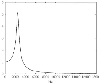
This difference equation keeps the propertyh(0)=0. Figure 6shows the frequency response of this approxi-mated reed model (solid line) superimposed with the exact one (dotted line).
This discrete reed model is stable under the condi-tion ωr < fe
4−q2
r. Under this condition, the mod-ulus of the poles of the transfer function is given by
(2fe−ωrqr)/(2fe+ωrqr) and is always smaller than 1. This
0 2000 4000 6000 8000 10000 12000 14000 16000 18000 Hz
Figure6: Approximated (solid line) and exact (dotted line) reed frequency response with parameter values fr =2500 Hz,qr =0.2, and fe=44.1 kHz.
stability condition makes this discretization scheme unsuit-able for use at low sampling rates, but in practice, at the CD quality sample rate, this problem does not arise for a reed res-onance frequency of up to 5 kHz with a quality factor of up to 0.5. For a more detailed discussion of discretization schemes, readers can consult, for example, [14].
The bilinear transformation does not provide a suitable discretization scheme for the reed displacement. In this case, the impulse response does not satisfy the property of the con-tinuous modelh(0)=0.
3.2. Impedance
A time domain equivalent to the inverse Fourier transform of impedanceZe(ω) given by (30) is now required. Here we expresspe(n) as a function ofue(n).
The losses in the cylindrical bore element contributing to the impedance of the whole bore are modeled with a digi-tal low-pass filter. This filter approximates the back and forth losses described byF(ω)2=exp(−2ik(ω)L) and neglects the
(small) dispersion. So that they can be adjusted to the ge-ometry of the resonator, the coefficients of the filter are ex-pressed analytically as functions of the physical parameters, rather than using numerical approximations and minimiza-tions. For this purpose, a one-pole filter is used,
˜
F( ˜ω)= b0exp(−iωD˜ )
1−a1exp(−iω˜)
, (41)
where ˜ω=ω/ fe, andD= 2fe(L/c) is the pure delay corre-sponding to a back and forth path of the waves.
The parameters b0 and a1 are calculated so that
|F(ω)2|2 = |F˜( ˜ω)|2 for two given values ofω, and are
so-lutions of the system
where |F(ω(1,2))2|2 = exp(−2ηc
ω(1,2)/2L). The first value
ω1 is an approximation of the frequency of the first
impedance peak of the truncated conical bore given byω1=
c(12πL+9π2x
e+16L)/(4L(4L+3πxe+4xe)), in order to ensure a suitable height of the impedance peak at the fundamental frequency. It is important to keep this feature to obtain a real-istic digital simulation of the continuous dynamical system, since the linear impedance is associated with the nonlinear characteristics. This ensures that the decay time of the fun-damental frequency of the approximated impulse response of the impedance matches the exact value, which is impor-tant in the case of fast changes in γ(e.g., attack transient). The second valueω2corresponds to the resonance frequency
of the Helmholz resonatorω2=c
S1/(L1V).
The phase of ˜F( ˜ω) has a nonlinear part, which is given by−arctan(a1sin( ˜ω)/(1−a1cos( ˜ω))). This part differs from
the nonlinear part of the phase of F(ω)2, which is given by
−ηc√ω/2L. Although these two quantities are different and
although the phase of ˜F( ˜ω) is determined by the choice of
a1, which is calculated from the modulus, it is worth
not-ing that in both cases, the dispersion is always very small, has a negative value, and is monotonic up to the frequency (fe/2π) arccos(a1). Consequently, in both cases, in the case of
a cylindrical bore, up to this frequency, the distance between successive impedance peaks decreases as their rank increases,
ωn+1−ωn< ωn−ωn−1.
Using (19) and (41), the impedance of the cylindrical bore unitC(ω) is then expressed by
C(z)= 1−a1z−1−b0z−D
1−a1z−1+b0z−D.
(43)
SinceL1is small, the frequency-dependent functionG(ω)
involved in the definition of the impedance of the short back-boreC1(ω) can be approximated by a constant,
correspond-ing to its value inω2.
The bilinear transformation is used to discretizeD=iω:
D(z)=2fe((z−1)/(z+ 1)).
The combination of all these parts according to (30) yields the digital impedance of the whole bore in the form
Ze(z)=
k=4
k=0bckz−k+ k=3
k=0bcDkz−D−k
1−k=4
k=1ackz−k− k=3
k=0acDkz−D−k
, (44)
where the coefficientsbck,ack,bcDk, andacDkare expressed
an-alytically as functions of the geometry of each part of the bore. This leads directly to the difference equation, which can be conveniently written in the form
pe(n)=bc0ue(n) + ˜V, (45) where ˜V includes all the terms that do not depend on the time samplen
˜
V= k=4
k=1
bckue(n−k) +
k=3
k=0
bcDkue(n−D−k)
+ k=4
k=1
ackpe(n−k) +
k=3
k=0
acDkpe(n−D−k).
(46)
0 500 1000 1500 2000 2500 3000 3500 4000 Hz
0 5 10 15 20 25 30
(a)
0 200 400 600 800 1000 1200 1400 1600 1800 2000 samples
−0.2
−0.1 0 0.1 0.2 0.3
(b)
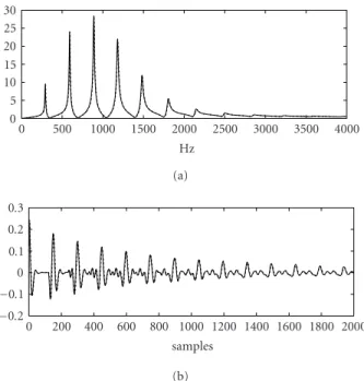
Figure7: (a) represents approximated (solid lines) and exact (dot-ted lines) input impedance, while (b) represents approxima(dot-ted (solid lines) and exact (dotted lines) impulse response. Geometri-cal parametersL=0.46 m,R=0.00216 m,θ =2◦,L1 =0.02 m,
R1=0.0015 m, andRb=0.006 m.
Figure 7shows an oboe-like bore input impedance, both approximated (solid line) and exact (dotted line) together with the corresponding impulse responses.
3.3. Synthesis algorithm
The sampled expressions for the impulse responses of the reed displacement and the impedance models are now used to write the sampled equivalent of the system of (31), (32), and (33):
x(n)=b1a
pe(n−1) +Ψβuue(n−1)2
+a1ax(n−1) +a2ax(n−2),
(47)
pe(n)=bc0ue(n) + ˜V, (48)
ue(n)=Wsign
γ−pe(n)γ−pe(n), (49) whereWis
W=Θ1−γ+x(n)
× ζ
1−γ+x(n)
1 +Ψβx
1−γ+x(n)2.
(50)
require pe(n) and ue(n) to be known. This makes it possi-ble to solve this system explicitly, as shown in [6], thus doing away with the need for schemes such as theK-method [15].
SinceWis always positive, if one considers the two cases
γ−pe(n)≥0 andγ−pe(n)<0, successively, substituting the expression forpe(n) from (48) into (49) eventually gives
ue(n)=1
2sign(γ−V˜) × −bc0W2+W
bc0W
2
+ 4|γ−V˜|
.
(51)
The acoustic pressure and flow in the mouthpiece at sam-pling timenare then finally obtained by the sequential cal-culation of ˜V with (46),x(n) with (47),Wwith (50),ue(n) with (51), andpe(n) with (48).
The external pressure pext(n) is calculated using the
dif-ference between the sum of the internal pressure and the flow at sampling timenandn−1.
4. SIMULATIONS
The effects of introducing the confined air jet into the non-linear characteristics are now studied in the case of two dif-ferent bore geometries. In particular, we consider a cylindri-cal resonator, the impedance peaks of which are odd har-monics, and a resonator, the impedance of which contains all the harmonics. We start by checking numerically the va-lidity of the resolution scheme in the case of the cylindrical bore. (Sound examples are available at http://omicron.cnrs-mrs.fr/∼guillemain/eurasip.html.)
4.1. Cylindrical resonator
We first consider a cylindrical resonator, and make the pa-rameter Ψ vary linearly from 0 to 4000 during the sound synthesis procedure (1.5 seconds). The transient attack cor-responds to an abrupt increase inγatt=0. During the de-cay phase, starting at t = 1.3 seconds,γdecreases linearly towards zero. Its steady-state value isγ = 0.56. The other parameters are constant, ζ = 0.35, βx = 7.5.10−4,βu = 6.1.10−3. The reed parameters areω
r =2π.3150 rad/second,
qr = 0.5. The resonator parameters are R = 0.0055 m,
L=0.46 m.
Figure 8shows superimposed curves, in the top figure, the digital impedance of the bore is given in dotted lines, and the ratio between the Fourier transforms of the sig-nalspe(n) andue(n) in solid lines; in the bottom figure, the digital reed transfer function is given in dotted lines, and the ratio of the Fourier transforms of the signalsx(n) and
pe(n) +Ψ(n)βuue(n)2(including attack and decay transients) in solid lines.
As we can see, the curves are perfectly superimposed. There is no need to check the nonlinear relation between
ue(n), pe(n), and x(n), which is satisfied by construction sinceue(n) is obtained explicitly as a function of the other variables in (51). In the case of the oboe-like bore, the re-sults obtained using the resolution scheme are equally accu-rate.
0 500 1000 1500 2000 2500 3000 3500 40004000 Hz
0 5 10 15 20 25 30
(a)
0 500 1000 1500 2000 2500 3000 3500 40004000 Hz
1 1.5 2
(b)
Figure8: (a) represents impedance (dotted line) and ratio between the spectra ofpeandue(solid line), while (b) represents reed trans-fer (dotted line) and ratio of spectra betweenxandpe+Ψβuu2
e(solid line).
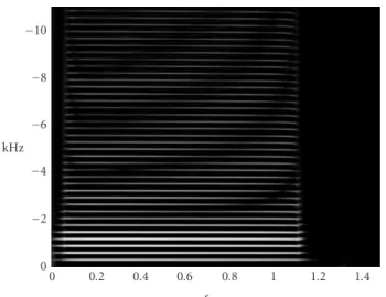
0 0.2 0.4 0.6 0.8 1 1.2 1.4 s
0
−2
−4
−6
−8
−10
kHz
Figure9: Spectrogram of the external pressure for a cylindrical bore and a beating reed whereγ=0.56.
4.1.1. The case of the beating reed
The first example corresponds to a beating reed situation, which is simulated by choosing a steady-state value of γ
greater than 0.5 (γ=0.56).
−8 −6 −4 −2 0 2 4 6 ×10⁻¹
0 2 4 6 8 10 12 14 16 18
×10−2
(a)
−8 −6 −4 −2 0 2 4 6
×10−1
0 2 4 6 8 10 12 14 16 18
×10−2
(b)
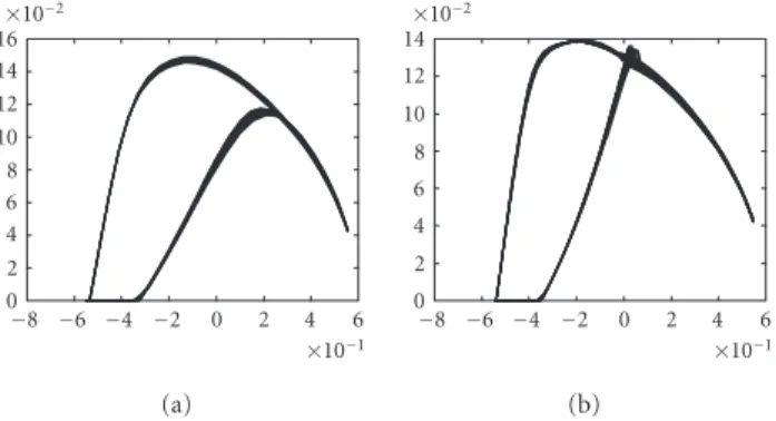
Figure 10:ue(n) versus pe(n): (a)t = 0.25 second, (b)t = 0.5 second.
−8 −6 −4 −2 0 2 4 6
×10−1
0 2 4 6 8 10 12 14 16
×10−2
(a)
−8 −6 −4 −2 0 2 4 6
×10−1
0 2 4 6 8 10 12 14
×10−2
(b)
Figure11:ue(n) versuspe(n): (a)t=0.75 second, (b)t=1 second.
Increasing the value of Ψ mainly affects the pitch and only slightly affects the amplitudes of the harmonics. In par-ticular, at high values ofΨ, a small increase inΨresults in a strong decrease in the pitch.
A cancellation of the self-oscillation process can be ob-served at aroundt=1.2 seconds, due to the high value ofΨ, since it occurs beforeγstarts decreasing.
Odd harmonics have a much higher level than even har-monics as occuring in the case of the clarinet. Indeed, the even harmonics originate mainly from the flow, which is taken into account in the calculation of the external pressure. However, it is worth noticing that the level of the second har-monic increases withΨ.
Figures10and11show the flowue(n) versus the pressure
pe(n), obtained during a small number (32) of oscillation pe-riods at aroundt=0.25 seconds,t=0.5 seconds,t=0.75 seconds and t = 1 seconds. The existence of two different paths, corresponding to the opening or closing of the reed, is due to the inertia of the reed. This phenomenon is observed also on single-reed instruments (see, e.g., [14]). A disconti-nuity appears in the whole path because the reed is beating. This cancels the opening (and hence the flow) while the pres-sure is still varying.
The shape of the curve changes with respect toΨ. This shape is in agreement with the results presented in [5].
0 0.2 0.4 0.6 0.8 1 1.2 1.4 s
0
−2
−4
−6
−8
−10
kHz
Figure12: Spectrogram of the external pressure for a cylindrical bore and a nonbeating reed whereγ=0.498.
−5−4−3−2−1 0 1 2 3 4 5 ×10⁻¹
0 2 4 6 8 10 12 14 16
×10−2
(a)
−5−4−3−2−1 0 1 2 3 4 5 ×10⁻¹
0 2 4 6 8 10 12 14 16
×10−2
(b)
Figure 13:ue(n) versus pe(n): (a)t = 0.25 second, (b)t = 0.5 second.
4.1.2. The case of the nonbeating reed
The second example corresponds to a nonbeating reed situa-tion, which is obtained by choosing a steady-state value ofγ
smaller than 0.5 (γ=0.498).
Figure 12shows the spectrogram of the external pressure generated by the model. Increasing the value ofΨresults in a sharp change in the level of the high harmonics at around
t=0.4 seconds, a slight change in the pitch, and a cancella-tion of the self-oscillacancella-tion process at aroundt=0.8 seconds, corresponding to a smaller value ofΨthan that observed in the case of the beating reed.
Figure 13shows the flowue(n) versus the pressurepe(n) at around t =0.25 seconds andt =0.5 seconds. Since the reed is no longer beating, the whole path remains continu-ous. The changes in its shape with respect toΨare smaller than in the case of the beating reed.
4.2. Oboe-like resonator
0 0.5 1 1.5 s
−0.4
−0.2 0 0.2 0.4
(a)
0 500 1000 1500 2000 2500 3000 3500 4000 samples
−0.2
−0.1 0 0.1 0.2
(b)
0 500 1000 1500 2000 2500 3000 3500 4000 samples
−0.1
−0.05 0 0.05 0.1
(c)
Figure 14: (a) represents external acoustic pressure, and (b), (c) represent attack and decay transients.
the input impedance, and geometric parameters of which correspond toFigure 7. The other parameters have the same values as in the case of the cylindrical resonator, and the steady-state value ofγisγ=0.4.
Figure 14shows the pressurepext(t). Increasing the effect
of the air jet confinement withΨ, and hence the aerodynam-ical losses, results in a gradual decrease in the signal ampli-tude. The change in the shape of the waveform with respect toΨcan be seen on the blowups corresponding to the attack and decay transients.
Figure 15shows the spectrogram of the external pressure generated by the model.
Since the impedance includes all the harmonics (and not only the odd ones as in the case of the cylindrical bore), the output pressure also includes all the harmonics. This makes for a considerable perceptual change in the timbre in comparison with the cylindrical geometry. Since the in-put impedance of the bore is not perfectly harmonic, it is not possible to determine whether the “moving formants” are caused by a change in the value ofΨor by a “phasing effect” resulting from the slight inharmonic nature of the impedance.
Increasing the value ofΨaffects the amplitude of the har-monics and slightly changes the pitch. In addition, as in the case of the cylindrical bore with a nonbeating reed, a large value ofΨbrings the self-oscillation process to an end.
0 0.2 0.4 0.6 0.8 1 1.2 1.4 s
0
−2
−4
−6
−8
−10
kHz
Figure15: Spectrogram of the external pressure for an oboe-like bore whereγ=0.4.
−16 −12 −8 −4 0 4
×10−1
0 2 4 6 8 10 12 14 16 18
×10−2
(a)
−14 −10 −6 −2 2
×10−1
0 2 4 6 8 10 12 14 16 18
×10−2
(b)
Figure 16:ue(n) versus pe(n): (a)t = 0.25 second, (b)t = 0.5 second.
−12 −8 −4 0 4
×10−1
0 2 4 6 8 10 12 14 16 18×
10−2
(a)
−10 −8 −6 −4 −2 0 2 4 ×10⁻¹
0 2 4 6 8 10 12 14 16×
10−2
(b)
Figure17:ue(n) versuspe(n): (a)t=0.75 second, (b)t=1 second.
Figures16and17show the flowue(n) versus the pressure
5. CONCLUSION
The synthesis model described in this paper includes the for-mation of a confined air jet in the embouchure of double-reed instruments. A dimensionless physical model, the form of which is suitable for transposition to a digital synthesis model, is proposed. The resonator is modeled using a time domain equivalent of the input impedance and does not re-quire the use of wave variables. This facilitates the model-ing of the digital couplmodel-ing between the bore, the reed and the nonlinear characteristics, since all the components of the model use the same physical variables. It is thus possible to obtain an explicit resolution of the nonlinear coupled sys-tem thanks to the specific discretization scheme of the reed model. This is applicable to other self-oscillating wind in-struments using the same flow model, but it still requires to be compared with other methods.
This synthesis model was used in order to study the in-fluence of the confined jet on the sound generated, by carry-ing out a real-time implementation. Based on the results of informal listening tests with an oboe player, the sound and dynamics of the transients obtained are fairly realistic. The simulations show that the shape of the resonator is the main factor determining the timbre of the instrument in steady-state parts, and that the confined jet plays a role at the con-trol level of the model, since it increases the oscillation step and therefore plays an important role mainly in the transient parts.
ACKNOWLEDGMENTS
The author would like to thank Christophe Vergez for helpful discussions on the physical flow model, and Jessica Blanc for reading the English.
REFERENCES
[1] R. T. Schumacher, “Ab initio calculations of the oscillation of a clarinet,”Acustica, vol. 48, no. 71, pp. 71–85, 1981. [2] J. O. Smith III, “Principles of digital waveguide models of
musical instruments,” inApplications of Digital Signal Pro-cessing to Audio and Acoustics, M. Kahrs and K. Branden-burg, Eds., pp. 417–466, Kluwer Academic Publishers, Boston, Mass, USA, 1998.
[3] V. V¨alim¨aki and M. Karjalainen, “Digital waveguide modeling of wind instrument bores constructed of truncated cones,” in
Proc. International Computer Music Conference, pp. 423–430, Computer Music Association, San Francisco, 1994.
[4] M. van Walstijn and M. Campbell, “Discrete-time modeling of woodwind instrument bores using wave variables,”Journal of the Acoustical Society of America, vol. 113, no. 1, pp. 575– 585, 2003.
[5] C. Vergez, R. Almeida, A. Causs´e, and X. Rodet, “Toward a simple physical model of double-reed musical instruments: influence of aero-dynamical losses in the embouchure on the coupling between the reed and the bore of the resonator,”
Acustica, vol. 89, pp. 964–974, 2003.
[6] Ph. Guillemain, J. Kergomard, and Th. Voinier, “Real-time synthesis of wind instruments, using nonlinear physical mod-els,” submitted to Journal of the Acoustical Society of Amer-ica.
[7] J. Kergomard, “Elementary considerations on reed-instru-ment oscillations,” in Mechanics of Musical Instruments, A. Hirschberg, J. Kergomard, and G. Weinreich, Eds., Springer-Verlag, New York, NY, USA, 1995.
[8] A. Almeida, C. Vergez, R. Causs´e, and X. Rodet, “Physical study of double-reed instruments for application to sound-synthesis,” inProc. International Symposium in Musical Acous-tics, pp. 221–226, Mexico City, Mexico, December 2002. [9] A. Hirschberg, “Aero-acoustics of wind instruments,” in
Me-chanics of Musical Instruments, A. Hirschberg, J. Kergomard, and G. Weinreich, Eds., Springer-Verlag, New York, NY, USA, 1995.
[10] S. Ollivier, Contribution `a l’´etude des oscillations des instru-ments `a vent `a anche simple, Ph.D. thesis, l’Universit´e du Maine, France, 2002.
[11] T. A. Wilson and G. S. Beavers, “Operating modes of the clar-inet,” Journal of the Acoustical Society of America, vol. 56, no. 2, pp. 653–658, 1974.
[12] Ph. Guillemain, J. Kergomard, and Th. Voinier, “Real-time synthesis models of wind instruments based on physical mod-els,” inProc. Stockholm Music Acoustics Conference, Stock-holm, Sweden, 2003.
[13] A. D. Pierce, Acoustics—An Introduction to Its Physical Prin-ciples and Applications, McGraw-Hill, New York, NY, USA, 1981, reprinted by Acoustical Society of America, Woodbury, NY, USA, 1989.
[14] F. Avanzini and D. Rocchesso, “Efficiency, accuracy, and sta-bility issues in discrete time simulations of single reed instru-ments,” Journal of the Acoustical Society of America, vol. 111, no. 5, pp. 2293–2301, 2002.
[15] G. Borin, G. De Poli, and D. Rocchesso, “Elimination of delay-free loops in discrete-time models of nonlinear acoustic sys-tems,” IEEE Trans. Speech and Audio Processing, vol. 8, no. 5, pp. 597–605, 2000.
Ph. Guillemainwas born in 1967 in Paris. Since 1995, he has been working as a full time researcher at the Centre National de la Recherche Scientifique (CNRS) in Mar-seille, France. He obtained his Ph.D. in 1994 on the additive synthesis modeling of natural sounds using time frequency and wavelets representations. Since 1989, he has been working in the field of musical sounds analysis, synthesis and transformation