Design of Stabilizing PI Controller for Coupled Tank MIMO Process

Volume 3, Issue 10 (September 2012), PP. 47-55

Design of Stabilizing PI Controller for Coupled Tank MIMO

Process

M.Senthilkumar

, Dr.S.Abraham Lincon

1,2

Electronics and Instrumentation Engineering, Annamalai University, Annamalainagar, Chidambaram-608002, India

Abstract––In this paper a new method is proposed for calculation of all stabilizing PI controllers for coupled tank multi-input multi-output (MIMO) process. By plotting the stability boundary locus in the (kp,ki) plane for coupled tank multivariable process after applying the decoupling technique, the stabilizing PI controller parameters are computed. The technique proposed does not require sweeping over the parameters and also does not need linear programming t o solve set of inequalities. This method is also used to obtain the all stabilizing PI controllers which achieve user specified gain and phase margins.

Keywords––MIMO, Coupled tank, Boundary locus, Stabilization, Decoupler

I.

INTRODUCTION

Designing stabilizing PI, PID and lag/lead controllers is of great importance for researchers since these controllers are popular and extensively used in process industries because of their performance and simplicity. Several methods are available to determine the controller parameters among them Zeigler –Nichols method and Cohen – Coon method are still widely used. After the work of Ho et al. [2], [3] the design of stabilizing P,PI and PID controller get more popular. For design of robust controller by computation of the stability region using the stability boundary locus has been given in [5]. All of these methods have been dealt with controller design applied to single- input single – output (SISO) systems. However in most of the processes more than one variable has to be controlled. These processes are called multi-input multi-output (MIMO) process. The control of these processes is more difficult than SISO processes. Because there is an interaction between other control loops of MIMO processes. Therefore the method used for SISO systems cannot use for control of MIMO systems effectively. Usually two types of control schemes are available to control MIMO processes. The first is decentralized control scheme or multiloop control scheme, where single loop controllers are used (the controller matrix is a diagonal one). The second scheme is a full multivariable controller (known as the centralized controller), where the controller matrix is not a diagonal one. Because of the interaction exist between the loops it is more difficult to design a stabilizing controller for MIMO process.

In this paper computation of stabilizing controller using the stability boundary locus method is applied to coupled tank multivariable process. First the decoupler is designed to eliminate the interaction between the loops and stabilizing values of PI controller is obtained in the parameter plane (Kp, Ki) for coupled tank process. The proposed method is also used for computation of PI controllers for achieving user defined gain and phase margins.

The paper is organized as follows: in section 2 computation of stabilizing PI controllers using stability boundary locus method is described. In section3 introduction about the decoupling technique is given. The coupled tank MIMO process is summarized in section 4. Computation of stabilizing PI controller and response for the coupled tank process is given in section 5.

II.

DETERMINATION OF STABILIZING PI CONTROLLERS

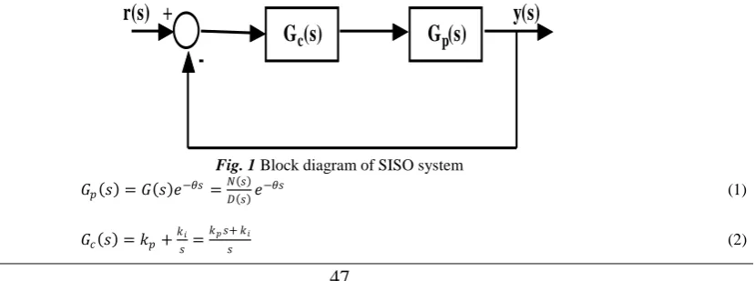
A possible approach to calculation of stabilizing PI controllers based on plotting the stability boundary locus is proposed in [Tan & kaya, 2003; Tan et al., 2006]. Consider the single-input single-output process as shown in Fig. 1 where Gp(s) is the process to be controlled by the PI controller Gc(s)

G

(s)

G

(s)

+

-r(s)

y(s)

Fig. 1 Block diagram of SISO system 𝐺𝑝 𝑠 = 𝐺 𝑠 𝑒−𝜃𝑠 =

𝑁 𝑠

𝐷 𝑠 𝑒

−𝜃𝑠 ₍₁₎

𝐺𝑐 𝑠 = 𝑘𝑝+

𝑘𝑖

𝑠 =

𝑘𝑝𝑠+ 𝑘𝑖

N(s) and D(s) are the numerator and denominator polynomial of the process by decomposing it into their corresponding even and odd part by replacing s by jω gives

𝐺 𝑗𝜔 =𝑁𝑒 −𝜔2 + 𝑗𝜔 𝑁𝑜(−𝜔2)

𝐷𝑒 −𝜔2 + 𝑗𝜔 𝐷𝑜(−𝜔2) (3)

For simplicity (-ω2) will be neglected in the following equation. The closed loop characteristic polynomial can be written as

∆ 𝑗𝜔 = 𝑘𝑖𝑁𝑒− 𝑘𝑝𝜔2𝑁0 cos 𝜔𝜃 + 𝜔(𝑘𝑖𝑁0+ 𝑘𝑝𝑁𝑒)sin 𝜔𝜃 − 𝜔2𝐷0 + 𝑗 [𝜔(𝑘𝑖𝑁0

+ 𝑘𝑝𝑁𝑒) cos 𝜔𝜃 − (𝑘𝑖𝑁𝑒− 𝜔2𝑘𝑝𝑁0) sin 𝜔𝜃 + 𝜔𝐷𝑒]

= 𝑅Δ+ 𝑗𝐼Δ= 0 (4) Equating the real and imaginary parts of Δ (jω) to zero we get

𝑘𝑝[−𝜔2𝑁𝑜cos 𝜔𝜃 + 𝜔𝑁𝑒sin(𝜔𝜃)] + 𝑘𝑖[𝑁𝑒cos 𝜔𝜃 + 𝜔𝑁𝑜sin(𝜔𝜃)] = 𝜔2𝐷𝑜 (5) 𝑘𝑝[𝜔𝑁𝑒 cos 𝜔𝜃 + 𝜔2𝑁0sin(𝜔𝜃)] + 𝑘𝑖[𝜔𝑁0cos 𝜔𝜃 − 𝑁𝑒sin(𝜔𝜃)] = −𝜔𝐷𝑒 (6) Solving equation (5) and (6) for kp and ki

𝑘𝑝 =

𝜔2_𝑁

0𝐷0+𝑁𝑒𝐷𝑒 cos 𝜔𝜃 +𝜔 𝑁0𝐷𝑒−𝑁𝑒𝐷0 sin 𝜔𝜃

− 𝑁𝑒2+ 𝜔2𝑁02

(7)

And

𝑘𝑖=

𝜔2_(𝑁

0𝐷𝑒−𝑁𝑒𝐷0) cos 𝜔𝜃 −𝜔 (𝑁𝑒𝐷𝑒+𝜔2𝑁0𝐷0) sin (𝜔𝜃 )

−(𝑁𝑒2+𝜔2𝑁02)

(8)

The stability boundary locus l(kp,ki,ω) in the(kp,ki)-plane can be obtained using equations (7) and (8).

From equations (7) and (8) it is observed that the stability boundary locus depend on the frequency ω which varies from 0 to ∞. Since the controller operates at the frequency range of below the critical frequency ωcor ultimate frequency , the stability boundary locus can be obtained over the frequency range of ω varies between 0 to ωc.

The performance of the controller can be evaluated by measuring the phase and gain margin. These two are the important frequency domain performance measure. Let the gain-phase margin tester𝐺𝑐 𝑠 = 𝐵𝑒−𝑗𝜙, which is connected in the feed forward path of the control system shown in Fig 1. Then the equation for kp and ki are

𝑘𝑝 =

𝜔2_𝑁

0𝐷0+𝑁𝑒𝐷𝑒 cos ℎ +𝜔 (𝑁0𝐷𝑒−𝑁𝑒𝐷0) sin (ℎ)

−𝐵(𝑁𝑒2+𝜔2𝑁02) (9)

𝑘𝑖 =𝜔

2_(𝑁

0𝐷𝑒−𝑁𝑒𝐷0) cos ℎ −𝜔 (𝑁𝑒𝐷𝑒+𝜔2𝑁0𝐷0) sin (ℎ)

−𝐵(𝑁𝑒2+𝜔2𝑁02)

(10)

Whereℎ = 𝜔𝜃 + 𝜙

One needs to set 𝜙 = 0 in (9) and (10) to obtain stability boundary locus for a given value of gain margin B. On the other hand by setting B=1 in the equation for kp and ki one can obtain the stability boundary locus for the given phase margin 𝜙

III.

DECOUPLING

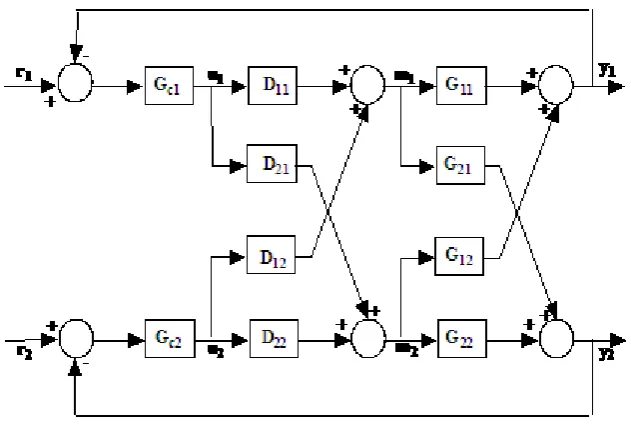
The problem with control-loop interaction is an important issue in MIMO process. The interaction occurs because one manipulated input affects more than one controlled output. One approach to handling this problem is decoupling. A simplified decoupling, is shown for a multivariable process is shown in Fig 2. Here the decoupling matrix is restricted with D11(s) = D22(s) =1 to the form

D(s) = 𝐷11(𝑠) 𝐷12(𝑠)

𝐷21(𝑠) 𝐷22(𝑠) (11) Here we specify a decoupled response and the decoupler with the structure in Equation

𝐺𝑃 𝑠 𝐷(𝑠) =

𝐺11(𝑠) 0

0 𝐺22(𝑠) (12)

𝐺11(𝑠) 𝐺12(𝑠)

𝐺21(𝑠) 𝐺22(𝑠)

1 𝐷12(𝑠)

𝐷21(𝑠) 1 =

𝐺11∗(𝑠) 0

0 𝐺22∗ (𝑠) And we can solve four equations in four unknowns to find

𝐷12 𝑠 = −

𝐺12 𝑠

𝐺11 𝑠

𝐷21 𝑠 = −

𝐺21(𝑠)

𝐺22(𝑠)

𝐺𝑙1(𝑠) = 𝐺11 𝑠 −

𝐺12 𝑠 𝐺21 𝑠

𝐺22 𝑠 (13)

𝐺𝑙2 𝑠 = 𝐺22 𝑠 −𝐺21

𝑠 𝐺12(𝑠)

𝐺11(𝑠) (14)

Fig. 2 Decentralized PI controller for MIMO process with decoupler

IV.

COUPLED TANK MIMO PROCESS

The schematic diagram of coupled tank MIMO process is shown in Fig.3. The input flows of tank1 and tank2 are Fin1 and Fin2. The controlled variables are level h1 and h2 in the tank1 and tank2.

The mass balance and Bernoulli’s law yield 𝐴𝑑ℎ1

𝑑𝑡 = 𝑘1𝑢1− 𝛽1𝑎1 2𝑔𝐻1− 𝛽𝑥𝑎12 2𝑔(𝐻1− 𝐻2) (15)

𝐴𝑑ℎ2

𝑑𝑡 = 𝑘2𝑢2+ 𝛽𝑥𝑎12 2𝑔(𝐻1− 𝐻2)− 𝛽2𝑎2 2𝑔𝐻2 (16) Where

A1, A2 - Cross sectional area of tank1 and tank2 (cm2) a1 - Cross sectional area of output pipe in

tank2 (cm2)

a2 - Cross sectional area of output pipe in tank2 (cm2)

a12 - Cross sectional area of interaction pipe between tank1 and tank2 (cm2) h1, h2 - Water level of tank1 and tank2 (cm) Fin1 - Inflow of tank1 (cm

3 /sec) Fin2 - Inflow of tank2 (cm3/sec) Fout1 - Outflow of tank1 (cm

3 /sec) Fout2 - Outflow of tank2 (cm3/sec) u1 - Input voltage to pump1 (volts) u2 - Input voltage to pump2 (volts) βx - Valve ratio of jointed pipe between tank1 and tank2

h1

Fin1 _F

in2

h2

Fout1 _Fout2

x

1 2

A1 A2

Fig.3 The coupled tank MIMO process

TableI Parameters of Laboratory Coupled Tank MIMO Process

A1, A2 a1,a2, a12 β1 β2 βx

154 0.5 0.7498 0.8040 0.2245

TableII Operating Conditions of Laboratory Coupled Tank MIMO Process

u1 u2 h1 h2 k1 k2

2.5 2.0 18.32 12.23 33.336 25.002

The parameter values of the coupled tank process are given in Table I. The nominal operating conditions of the process are shown in Table II.

V.

SIMULATION AND EXPERIMENT RESULT

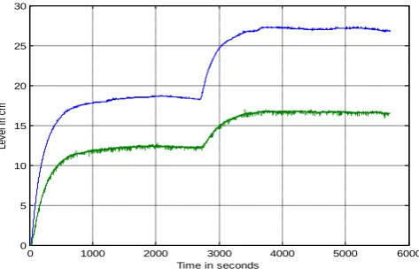
The transfer function model for the coupled tank process is identified using reaction curve method. The levels in the tanks are initially maintained at the operating condition of 18.32 cm and 12.23 cm by giving the input voltage of 2.5 and 2.0 volts to the pump1 and pump2 respectively. Then the input to pump1 is changed from 2.5 to 3.0 voltage by keeping pump 2 input constant and the level in tank 1 and tank2 are recorded. The same procedure is repeated by changing the pump2 input from 2.0 to 2.5 volts by keeping the pump1 input constant. The open loop response for the change in input1 and input2 are shown in Fig.4 and 5.The experimentally identified transfer function model is

𝐺𝑝 𝑠 =

16.99 𝑒−12.89𝑠

214.03𝑠 + 1

6.69 𝑒−72.57𝑠

204.93𝑠 + 1

9.23 𝑒−35.01𝑠

256.44𝑠 + 1

11.38 𝑒−25.04𝑠

169.15𝑠+1

(17)

This transfer function model is used to design a controller. After obtaining the decoupler Gl1 and Gl2 are calculated using eq(13) and (14) as

𝐺𝑙1 𝑠 =

11.56 𝑒−6.63𝑠

156.18𝑠+1 (18)

And

𝐺𝑙2 𝑠 =

7.745 𝑒−24.23𝑠

111.01𝑠+1 (19)

𝑘𝑖1= 13.51𝜔2cos 6.63𝜔 + 0.0865𝜔 sin(6.63𝜔) (21)

Similarly for 𝐺𝑙2(𝑠) 𝑘𝑝2= 14.33𝜔 sin 24.23𝜔 − 0.129 cos(24.23𝜔) (22)

𝑘𝑖2= 14.33𝜔2cos 24.23𝜔 + 0.129𝜔 sin(24.23𝜔) (23)

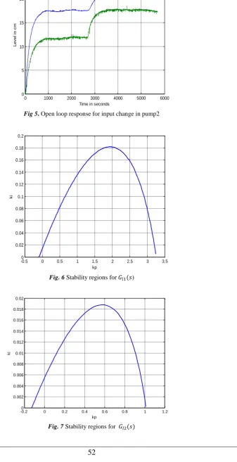
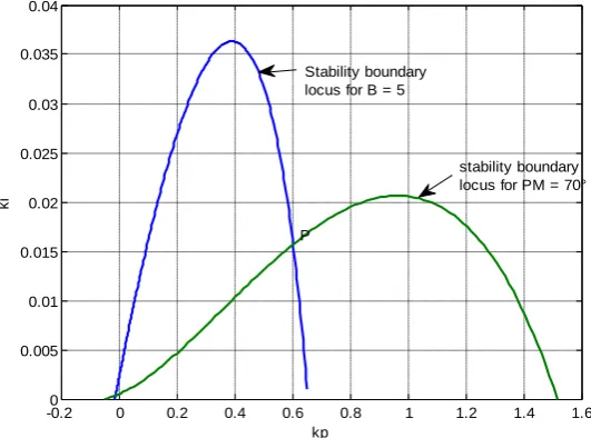
The stability boundary locus for 𝐺𝑙1(𝑠) and 𝐺𝑙2(𝑠) is plotted in kp – ki plane for 𝜔𝜖 0 1.2 and 𝜔𝜖 0 0.0702 respectively, which is shown in Fig .6 and Fig .7. To find all stabilizing PI controller for the phase margin of the system greater than 70° and gain margin is greater than 5 for both 𝐺𝑙1(𝑠) and 𝐺𝑙2(𝑠) . First set B=1 and 𝜙 = 70 in Eqs (9) and (10). Therefore 𝑘𝑝1= 13.51𝜔 sin ℎ − 0.0865 cos(ℎ) (24)

𝑘𝑖1= 13.51𝜔2cos ℎ + 0.0865𝜔 sin(ℎ) (25)

𝑘𝑝2= 14.33𝜔 sin ℎ − 0.129 cos(ℎ) (26)

𝑘𝑖2= 14.33𝜔2cos ℎ + 0.129𝜔 sin(ℎ) (27)

Where ℎ = 𝜔𝜃 + 70. Second to find the stabilizing PI controllers for the gain margin greater than 5 set B=5 and 𝜙 = 0 in Eqs (9) and (10). For𝐺𝑙1(𝑠), using (9) and (10) for these values of B and 𝜙 gives 𝑘𝑝1= 2.702𝜔 sin 6.63𝜔 − 0.0173 cos(6.63𝜔) (28)

𝑘𝑖1= 2.702𝜔2cos 6.63𝜔 + 0.0173𝜔 sin(6.63𝜔) (29) Similarly for 𝐺𝑙2(𝑠) 𝑘𝑝2= 2.866𝜔 sin 24.23𝜔 − 0.0258 cos(24.23𝜔) (30)

𝑘𝑖2= 2.866𝜔2cos 24.23𝜔 + 0.0258𝜔 sin(24.23𝜔) (31)

Thus the stabilizing PI controller’s boundary locus of 𝐺𝑙1(𝑠) and 𝐺𝑙2(𝑠) for 𝐵 ≥ 5 and𝜙 ≥ 70 are shown in Fig.8 and 9 respectively

Fig. 4Open loop response for input change in Pump1

0 1000 2000 3000 4000 5000 6000

0 5 10 15 20 25 30

Time in seconds

Le

ve

l i

n

Fig 5. Open loop response for input change in pump2

Fig. 6 Stability regions for 𝐺𝑙1(𝑠)

0 1000 2000 3000 4000 5000 6000

0 5 10 15 20 25

Time in seconds

L

e

v

e

l

in

c

m

-0.50 0 0.5 1 1.5 2 2.5 3 3.5

0.02 0.04 0.06 0.08 0.1 0.12 0.14 0.16 0.18 0.2

kp

ki

-0.20 0 0.2 0.4 0.6 0.8 1 1.2

0.002 0.004 0.006 0.008 0.01 0.012 0.014 0.016 0.018 0.02

kp

Fig. 8 Stabilizing PI controllers of 𝐺𝑙1(𝑠) for specified gain and phase margin

Fig.9 Stabilizing PI controllers of 𝐺𝑙2(𝑠) for specified gain and phase margins

-0.20 0 0.2 0.4 0.6 0.8 1 1.2 1.4 1.6

0.005 0.01 0.015 0.02 0.025 0.03 0.035 0.04

kp

ki

P

Stability boundary locus for B = 5

stability boundary locus for PM = 70°

-0.10 0 0.1 0.2 0.3 0.4 0.5 0.6

0.5 1 1.5 2 2.5 3 3.5 4 4.5

5x 10

-3

kp

ki

stability boundary locus for B =5

stability boundary locus for PM = 70°

0 500 1000 1500

18 20 22 24 26 28 30

Time in seconds

Le

ve

l i

n

Fig.10 Closed Loop Response for set Point change in Tank1 from 18.32 to 25 cm.

Fig. 11 Closed Loop Response for Tank2 for set Point change in Tank2 from 12.23 to 17 cm.

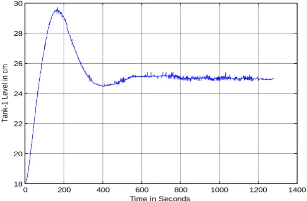
Fig. 12 Real Time Closed Loop Response for set Point change in Tank1 from 18.32 to 25 cm.

0 500 1000 1500

12 13 14 15 16 17 18

Time in seconds

Le

ve

l i

n

cm

0 200 400 600 800 1000 1200 1400

18 20 22 24 26 28 30

Time in Seconds

T

an

k-1

Le

ve

l i

n

cm

0 200 400 600 800 1000 1200 1400 1600 1800 2000

13 14 15 16 17 18 19 20 21

Ta

nk

-2

L

ev

el

in

c

The closed loop simulation response for setpoint change in tank1 and tank2 are shown in Fig. 11 and Fig.12with the controller parameters of kp1=0.606, ki1=0.0157 and kp2=0.1647, ki2=0.00287 .The real time responses are obtained using VDPID card for interface with the process with sampling time of 0.1 seconds and the closed loop responses are shown in Fig. 13 and 14.

VI.

CONCLUSIONS

In this paper, a method is proposed to design a PI controller for a coupled-tank multivariable process by plotting stability boundary locus. The PI controller is designed by equating the real and imaginary part of the characteristic equation of both the loop after applying decoupling to zero. The value for the controller is obtained with ease by plotting the stability boundary locus in Kp-Ki plane, without doing the linear programming to solve the set of inequalities. And also the PI controller parameters for the coupled -tank is obtained for the user defined gain and phase margin. The simulation and experimentation results presented clearly shows the value of the method.

REFERENCES

[1]. Astrom, K.J. and T.Hagglund,” The future of PID control, “Control Engineering Practice, vol.9, pp.1163-1175, 2001.

[2]. Ho, M.T., A.Datta and S.P.Bhattacharyya,” A new approach to feedback stabilization,’’ Proc.of the 35th CDC, pp4643-4648, 1996

[3]. Ho, M.T., A.Datta and S.P.Bhattacharyya.” A linear programming characterization of all stabilizing PID controllers,”Proc. Of Amer.Contr.Conf, 1997.

[4]. Soylemez. M.T.,N.Munro and H. Baki,”Fast calculation of stabilizing PID controllers,” Automatica, Vol.39,pp121-126,2003.

[5]. Tan,N.,I.Kaya and D.P.Atherton ,”computation of stabilizing PI and PID controllers,”Proc. Of the 2003 IEEE Intern. Conf. on the Control Applications (CCA2003), Istanbul, Turkey, 2003.

[6]. Tan .N,” computation of stabilizing PI and PID controllers for processes with time delay,”ISA Transaction, VOl.44.pp 213-223, 2005.

[7]. Tan, N., I.Kaya.C.Yeroglu andD.P.Atherton,”computation of stabilizing PI and PID controllers using the stability boundary locus,”Energy Conversion and management, Vol.47.pp3045-3058, 2006.

[8]. Zhaung, M .and D.P.Atherton,”PID controller design for a TITO system,”IEE Proc. Control Theory Appl., Vol.141, no.2, pp. 111-120, 1994.

[9]. Fang,J ., Da Zheng and ZhengyunRen ,” computation of stabilizing PI and PID controllers by using Kronecker summation method,”Energy Conversion and management ,Vol.50 .pp1821 -1827 ,2009.

[10]. R. Matušů, R. Prokop, K. Matejičková, and M. Bakošová, “Robust stabilization of interval plants using Kronecker summation method”WSEAS Transactions on Systems, vol. 9, no. 9, pp. 917-926, 2010.

[11]. Ho, M. T., A. Datta and S. P. Bhattacharyya, “A linear programming characterization of all stabilizing PID controllers,” Proc. of Amer. Contr. Conf., 1997.

[12]. Shafiei, Z. and A. T. Shenton, “Frequency domain design of PID controllers for stable and unstable systems with time delay,” Automatica, vol. 33, pp. 2223-2232, 1997.

[13]. Huang, Y. J. and Y. J. Wang, “Robust PID tuning strategy for uncertain plants based on the Kharitonov theorem,”