Similarity modeling for machine learning

(1)

c

(2)

SIMILARITY MODELING FOR MACHINE LEARNING

BY

YINGZHEN YANG

DISSERTATION

Submitted in partial fulfillment of the requirements

for the degree of Doctor of Philosophy in Electrical and Computer Engineering in the Graduate College of the

University of Illinois at Urbana-Champaign, 2016

Urbana, Illinois

Doctoral Committee:

Professor Thomas S. Huang, Chair Professor Mark Hasegawa-Johnson Professor Zhi-Pei Liang

(3)

ABSTRACT

Similarity is the extent to which two objects resemble each other. Modeling simi-larity is an important topic for both machine learning and computer vision. In this dissertation, we first propose a discriminative similarity learning method, then in-troduce two novel sparse similarity modeling methods for high dimensional data from the perspective of manifold learning and subspace learning. Our sparse similarity modeling methods learn sparse similarity and consequently generate a sparse graph over the data. The generated sparse graph leads to superior per-formance in clustering and semi-supervised learning, compared to existing sparse graph based methods such as`1_{-graph and Sparse Subspace Clustering (SSC).}

More concretely, our discriminative similarity learning method adopts a novel pairwise clustering framework by bridging the gap between clustering and multi-class multi-classification. This pairwise clustering framework learns an unsupervised nonparametric classifier from each data partition, and searches for the optimal partition of the data by minimizing the generalization error of the learned classi-fiers associated with the data partitions.

Regarding to our sparse similarity modeling methods, we propose a novel `0 regularized `1_{-graph (`}0_-`1_{-graph) to improve} _`1_{-graph from the perspective of} manifold learning. Our `0_-`1_{-graph generates a sparse graph that is aligned to} the manifold structure of the data for better clustering performance. From the perspective of learning the subspace structures of the high dimensional data, we propose `0_{-graph that generates a subspace-consistent sparse graph for} cluster-ing and semi-supervised learncluster-ing. Subspace-consistent sparse graph is a sparse graph where a data point is only connected to other data that lie in the same sub-space, and the representative method Sparse Subspace Clustering (SSC) proves to generate subspace-consistent sparse graph under certain assumptions on the subspaces and the data, e.g. independent/disjoint subspaces and subspace inco-herence/affinity. In contrast, our`0_{-graph can generate subspace-consistent sparse} graph for arbitrary distinct underlying subspaces under far less restrictive

(4)

assump-tions, i.e. only i.i.d. random data generation according to arbitrary continuous distribution. Extensive experimental results on various data sets demonstrate the superiority of `0_{-graph compared to other methods including SSC for both} clus-tering and semi-supervised learning.

The proposed sparse similarity modeling methods require sparse coding using the entire data as the dictionary, which can be inefficient especially in case of large-scale data. In order to overcome this challenge, we propose Support Regu-larized Sparse Coding (SRSC) where a compact dictionary is learned. The data similarity induced by the support regularized sparse codes leads to compelling clustering performance. Moreover, a feed-forward neural network, termed Deep-SRSC, is designed as a fast encoder to approximate the codes generated by Deep-SRSC, further improving the efficiency of SRSC.

(5)

(6)

ACKNOWLEDGMENTS

First, I would like to express my deep gratitude to my adviser Professor Thomas S. Huang for all of his guidance, advice, and support throughout my Ph.D. study at UIUC. It would be very difficult for me to devote most of my work time to my favorite and fundamental topics of statistical machine learning research with-out his enlightened attitude and support. During the past five and half years, I have been inspired by his vision, wisdom, passion and dedication to high-quality research and his respectful personality. The experience of working with him is undoubtedly an invaluable merit for my professional career in the future.

It has been a great honor for me to collaborate with Professor Feng Liang at the Department of Statistics of UIUC, Shuicheng Yan at National University of Singapore. I was deeply impressed by their profound insights into my research problems. I was lucky to work with Dr. Nebojsa Jojic as a summer intern at Mi-crosoft Research Redmond. From him, I learned research skills and how to view my research topics from different perspectives. I am very thankful to Dr. Push-meet Kohli at Microsoft Research Redmond for his suggestions on my research. I also appreciate the comments and advice from Professor Mark Hasegawa-Johnson and Professor Zhi-Pei Liang, and I am fortunate to have them as my thesis com-mittee members.

I would like to extend my appreciation to my mentor, Mr. Dan Gelb, for his suggestions and advice on my research project at Hewlett-Packard Laboratories during the summer of 2011. I also learned a lot of engineering skills from him. I greatly thank Dr. Jianchao Yang at Snapchat Research for his insightful comments and advice on my various research projects. I owe sincere gratitude to Professor Jiashi Feng at National University of Singapore. I also owe sincere thanks to many student collaborators including IFP members Wei Han, Zhaowen Wang, Jiangping Wang and Jiahui Yu, as well as Zhiding Yu from Carnegie Mellon University.

I would also like to extend my deepest gratitude to my family. Without their encouragement and unconditional love, life would not be so beautiful.

(7)

CHAPTER 1

INTRODUCTION

Similarity is the extent to which two objects resemble each other. Similarity mod-eling is regarded as one of the most important topics in machine learning with broad applications in computer vision exhibiting compelling performance in vari-ous learning and vision tasks. In this dissertation, we first propose a discriminative similarity learning method, then introduce two novel similarity modeling methods for general high dimensional data from the perspective of manifold learning and subspace learning with convincing theoretical and empirical results. We finally propose Support Regularized Sparse Coding, which learns a compact dictionary rather than using the entire data as the dictionary in the previous two methods.

A discriminative similarity learning method is proposed in Chapter 2, which adopts a new framework for pairwise clustering wherein the pairwise similarity is derived as the generalization error bound for the unsupervised nonparametric classifier. The unsupervised classifier is learned from unlabeled data and the hy-pothetical labeling. The quality of the hyhy-pothetical labeling is measured by the associated generalization error of the learned classifier, and the hypothetical la-beling with minimum associated generalization error bound is preferred. We con-sider two nonparametric classifiers, i.e. the nearest neighbor classifier (NN) and the plug-in classifier (or the kernel density classifier). The generalization error bounds for both unsupervised classifiers are expressed as sum of pairwise terms between the data points, which can be interpreted as nonparametric pairwise sim-ilarity measure between the data points. Under uniform distribution, both non-parametric similarity measures exhibit a well known form of kernel similarity. We also prove that the generalization error bound for the unsupervised plug-in classifier is asymptotically equal to the weighted volume of cluster boundary [1] for Low Density Separation, a widely used criterion for semi-supervised learning and clustering.

Sparse representation serves as the major tool for our sparse similarity modeling methods. Chapter 3 and 4 describe our similarity learning models that learn sparse

(10)

similarity and consequently generate a sparse graph over which superior cluster-ing and semi-supervised learncluster-ing performance are achieved. A sparse graph is a graph which has only a few edges of nonzero weights for each vertex, wherein the learned sparse similarity serves as the edge weight. Sparse graph is demonstrated to be effective for clustering and semi-supervised learning, especially for high dimensional data. Examples of sparse graph based machine learning methods in-clude `1-graph [2, 3] and Sparse Subspace Clustering (SSC) [4]. Our similarity learning models produce an improved sparse graph from the perspective of mani-fold learning and subspace learning.

More concretely, Chapter 3 describes similarity learning from the perspective of manifold learning. We propose a novel`0 _regularized_`1_{-graph (`}0_-`1_{-graph) to} improve`1_{-graph. Our}_`0_-`1_{-graph generates a sparse graph that is aligned to the} manifold structure of the data for better clustering performance based on manifold assumption [5, 6, 7, 8, 9]. `0_-`1_{-graph employs manifold assumption on the local} structure of the sparse graph, which requires that nearby data in the manifold are encouraged to have similar local sparse graph structure, i.e. they should have sim-ilar neighbors and simsim-ilar edge weights in the sparse graph. `0-`1-graph imposes such manifold assumption by using `0-distance between the sparse codes in the graph regularization term. We develop an iterative proximal method to solve the nonconvex optimization problem of `0_-`1_{-graph with proven guarantee of} con-vergence. Extensive experimental results on various real data sets demonstrate the superiority of`0_-`1_{-graph over other competing clustering methods including} `1_{-graph and its}_`2 _{regularized version, namely}_`2_-`1_-graph. _`2_-`1_{-graph uses}_`2 -distance for the sparse codes in the graph regularization term, a common choice adopted broadly in existing graph regularized sparse representation methods.

Chapter 4 describes similarity learning from the perspective of learning the subspace structures of the high dimensional data. We propose `0-graph, which generates subspace consistent sparse graph for clustering and semi-supervised learning. Sparse subspace learning methods, such as Sparse Subspace Cluster-ing (SSC), assume that the high dimensional data lie in a union of subspaces, and they aim to build a sparse graph where a data point is only connected to other data that lie in the same subspace. Such sparse graph is called subspace con-sistent sparse graph. Data belonging to different subspaces are disconnected in the subspace consistent sparse graph; therefore, compelling clustering and semi-supervised learning performance are achieved by applying standard graph based machine learning methods, such as spectral clustering [10] and label propagation

(11)

[11], over the subspace-consistent sparse graph. Most of sparse subspace cluster-ing methods require certain assumptions, e.g. independence or disjointness, on the subspaces to obtain the subspace consistent sparse graph. These assumptions are not guaranteed to hold in practice and they limit the application of existing sparse subspace learning methods on subspaces with general location. In this disserta-tion, we propose `0_{-graph, which obtains the subspace-consistent sparse graph} for arbitrary distinct underlying subspaces almost surely under the mild i.i.d. as-sumption on the data generation. Extensive experimental results on various data sets demonstrate the superiority of`0-graph over other methods including SSC for both clustering and semi-supervised learning.

The above two similarity modeling methods produce a sparse graph over the data using the entire data as the dictionary in the sparse approximation procedure. Therefore, their efficiency is hindered by the size of the data. In order to overcome this challenge, we propose Support Regularized Sparse Coding (SRSC) in Chap-ter 5, which learns a compact dictionary rather than using the entire data as the dictionary. In contrast to ordinary sparse coding where the sparse code with fixed dictionary is independent for each data point without considering the geometric information and manifold structure of the entire data, SRSC produces sparse code that accounts for the manifold structure of the data by encouraging nearby data in the manifold to choose similar dictionary atoms. In this way, the obtained support regularized sparse code captures the locally linear structure of the data manifold. The similarity of two data points is intuitively set to the positive part of the inner product of the corresponding support regularized sparse codes, leading to com-pelling clustering performance. Moreover, we design a novel feed-forward neural network named Deep Support Regularized Sparse Coding (Deep-SRSC) as a fast encoder to approximate the sparse code generated by SRSC. Instead of the or-dinary optimization method which requires time-consuming numerous iterations, Deep-SRSC outputs the support regularized sparse codes by feeding the data into a network which is comprised of only a few layers, and the architecture of the layer is designed in an interpretable way according to the optimization of SRSC. Experimental results on real data demonstrate the effectiveness of Deep-SRSC.

(12)

CHAPTER 2

ON A THEORY OF NONPARAMETRIC

PAIRWISE SIMILARITY FOR

CLUSTERING: CONNECTING

CLUSTERING TO CLASSIFICATION

2.1

Introduction

Pairwise clustering methods partition the data into a set of self-similar clusters based on the pairwise similarity between the data points. Representative cluster-ing methods include K-means [12] which minimizes the within-cluster dissimilar-ities, spectral clustering [10] which identifies clusters of more complex shapes ly-ing on low dimensional manifolds, and the pairwise clusterly-ing method [13] usly-ing message-passing algorithm to inference the cluster labels in a pairwise undirected graphical model. Utilizing pairwise similarity, these pairwise clustering methods often avoid estimating complex hidden variables or parameters, which is difficult for high dimensional data.

However, most pairwise clustering methods assume that the pairwise similarity is given [12, 10], or they learn a more complicated similarity measure based on several given base similarities [13]. In this chapter, we present a new framework for pairwise clustering where the pairwise similarity is derived as the generaliza-tion error bound for the unsupervised nonparametric classifier. The unsupervised classifier is learned from unlabeled data and the hypothetical labeling. The qual-ity of the hypothetical labeling is measured by the associated generalization error of the learned classifier, and the hypothetical labeling with minimum associated generalization error bound is preferred. We consider two nonparametric classi-fiers, i.e. the nearest neighbor classifier (NN) and the plug-in classifier (or the kernel density classifier). The generalization error bounds for both unsupervised classifiers are expressed as sum of pairwise terms between the data points, which can be interpreted as a nonparametric pairwise similarity measure between the data points. Under uniform distribution, both nonparametric similarity measures exhibit a well-known form of kernel similarity. We also prove that the general-ization error bound for the unsupervised plug-in classifier is asymptotically equal

(13)

to the weighted volume of cluster boundary [1] for Low Density Separation, a widely used criterion for semi-supervised learning and clustering.

Our work is closely related to discriminative clustering methods by unsuper-vised classification, which searches for the cluster boundaries with the help of an unsupervised classifier. For example, [14] learns a max-margin two-class classi-fier to group unlabeled data in an unsupervised manner, known as unsupervised SVM, whose theoretical property is further analyzed in [15]. Also, [16] learns the kernel logistic regression classifier, and uses the entropy of the posterior dis-tribution of the class label by the classifier to measure the quality of the learned classifier. More recent work presented in [17] learns an unsupervised classifier by maximizing the mutual information between cluster labels and the data, and the Squared-Loss Mutual Information is employed to produce a convex optimiza-tion problem. Although such discriminative methods produce satisfactory empir-ical results, the optimization of complex parameters hampers their application in high-dimensional data. Following the same principle of unsupervised classifica-tion using nonparametric classifiers, we derive nonparametric pairwise similarity and eliminate the need of estimating complicated parameters of the unsupervised classifier. As an application, we develop a new nonparametric exemplar-based clustering method with the derived nonparametric pairwise similarity induced by the plug-in classifier, and our new method demonstrates better empirical cluster-ing results than the existcluster-ing exemplar-based clustercluster-ing methods.

It should be emphasized that our generalization bounds are essentially different from the literature. As nonparametric classification methods, the generalization properties of the nearest neighbor classifier (NN) and the plug-in classifier are ex-tensively studied. Previous research focuses on the average generalization error of the NN [18, 19], which is the average error of the NN over all the random training data sets, or the excess risk of the plug-in classifier [20, 21]. In [18], it is shown that the average generalization error of the NN is bounded by twice the Bayes error. Assuming that the class of the regression functions has a smooth parame-ter β, [20] proves that the excess risk of the plug-in classifier converges to 0of the ordern2−β+βd wheredis the dimension of the data. [21] further shows that the

plug-in classifier attains faster convergence rate of the excess risk, namelyn−12, under some margin assumption on the data distribution. All these generalization error bounds depend on the unknown Bayes error. By virtue of kernel density esti-mation and generalized kernel density estiesti-mation [22], our generalization bounds are represented mostly in terms of the data, leading to the pairwise similarities for

(14)

clustering.

2.2

Formulation of Pairwise Clustering by

Unsupervised Nonparametric Classification

The discriminative clustering literature [14, 16] has demonstrated the potential of multi-class classification for the clustering problem. Inspired by the natural connection between clustering and classification, we model the clustering problem as a multi-class classification problem: a classifier is learned from the training data built by a hypothetical labeling, which is a possible cluster labeling. The optimal hypothetical labeling is supposed to be the one such that its associated classifier has the minimum generalization error bound. To study the generalization bound for the classifier learned from the hypothetical labeling, we define the concept of classification model. Given unlabeled data{xl}nl=1, a classification modelMY is

constructed for any hypothetical labelingY ={yl}nl=1as below:

Definition 1. The classification model corresponding to the hypothetical labeling

Y = {yl}nl=1 is defined asMY =

S, PXY,{πi, fi}Qi=1, F

. S ={xl,yl}nl=1 are

the labeled data by the hypothetical labeling, andS are assumed to be i.i.d. sam-ples drawn from the joint distributionPXY =PX|YPY, where(X, Y)is a random

couple,X ∈IRdrepresents the data andY ∈ {1,2, ..., Q}is the class label ofX,

Qis the number of classes determined by the hypothetical labeling. Furthermore,

PXY is specified by{π(i), f(i)}Qi=1as follows:π(i)is the class prior for classi, i.e.

Pr [Y =i] = π(i)_{; the conditional distribution} _P

X|Y=i has probabilistic density

function f(i)_, _i _{= 1}_{, . . . , Q}_. _F _{is a classifier trained using the training data}_S_.

The generalization error of the classification modelMY is defined as the general-ization error of the classifierF inMY.

In this chapter, we study two types of classification models with the nearest neighbor classifier and the plug-in classifier respectively, and derive their gen-eralization error bounds as sum of pairwise similarity between the data. Given a specific type of classification model, the optimal hypothetical labeling corre-sponds to the classification model with minimum generalization error bound. The optimal hypothetical labeling also generates a data partition where the sum of pairwise similarity between the data from different clusters is minimized, which is a common criterion for discriminative clustering.

(15)

In the following text, we derive the generalization error bounds for the two types of classification models. Before that, we introduce more notations and assump-tions for the classification model. Denote byPX the induced marginal distribution

of X, andf is the probabilistic density function ofPX which is a mixture ofQ

class-conditional densities: f =

Q

P

i=1

π(i)_f(i)_. _η(i)₍_x₎ _{is the regression function} of Y on X = x, i.e. η(i)₍_x_{) = Pr [}_Y ₌_i_|X ₌_x_{] =} π(i)_f(i)₍_x₎

f(x) . For the sake of the consistency of the kernel density estimators used in the sequel, there are further assumptions on the marginal density and class-conditional densities in the classification model for any hypothetical labeling:

(A)f is bounded from below, i.e.f ≥fmin>0.

(B){f(i)_}_{is bounded from above, i.e.}_f(i) _≤_f(i)

max, andf(i) ∈Σγ,ci,1≤i≤Q.

whereΣγ,c is the class of H¨older-γsmooth functions with H¨older constantc:

Σγ,c ,{f : IRd→IR| ∀x, y,|f(x)−f(y)| ≤ckx−ykγ}, γ >0

It follows from assumption (B) thatf ∈Σγ,cwherec=P i

π(i)_c

i. Assumptions

(A) and (B) are mild. The upper bound for the density functions is widely required for the consistency of kernel density estimators [23, 24]; H¨older-γ smoothness is required to bound the bias of such estimators, and it also appears in [21] for esti-mating the excess risk of the plug-in classifier. The lower bound for the marginal density is used to derive the consistency of the estimator of the regression func-tion η(i) _{(Lemma 2) and the consistency of the generalized kernel density} esti-mator (Lemma 3). We denote byPX the collection of marginal distributions that

satisfy assumption (A), and denote by PX|Y the collection of class-conditional

distributions that satisfy assumption (B). We then define the collection of joint distributions PXY thatPXY belongs to, which requires the marginal density and

class-conditional densities satisfy assumption (A)-(B):

P_XY _,{PXY |PX ∈ PX,{PX|Y=i} ∈ PX|Y,min i {π

(i)_}_>₀_} _(2.1) Given the joint distribution PXY, the generalization error of the classifier F

learned from the training dataS is:

R(FS),Pr [(X, Y) :F(X)6=Y] (2.2)

(16)

esti-mating the underlying probabilistic density functions in our generalization analy-sis, and we introduce the KDE off as follows:

ˆ fn,hn(x) = 1 n n X l=1 Khn(x−xl) (2.3) whereKh(x) = _h1dK x h

is the isotropic Gaussian kernel with bandwidthhand K(x)_, 1

(2π)d/2e

−kx₂k2_{. We have the following VC property of the Gaussian kernel}

K. Define the class of functions

F _,{K t− · h , t∈IRd, h6= 0} (2.4)

The VC property appears in [23, 24, 25, 26, 27], and it is proved that F is a bounded VC class of measurable functions with respect to the envelope function F such that|u| ≤F for anyu ∈ F (e.g. F ≡(2π)−d2). It follows that there exist positive numbers A and v such that for every probability measureP on IRd for whichRF2_{dP <}_∞_{and any}₀_{< τ <}₁_,

NF,k·k_L₂₍_P₎, τkFk_L₂₍_P₎≤ A τ v (2.5)

where NT,d, ˆ is defined as the minimal number of open d-balls of radiusˆ required to cover T in the metric space

T,dˆ. A and v are called the VC characteristics ofF.

The VC property ofKis required for the consistency of kernel density estima-tors shown in Lemma 2. Also, we adopt the following kernel estimator ofη(i):

ˆ η_n,h(i) n(x) = n P l=1 Khn(x−xl)1I{yl=i} nfˆn,hn(x) (2.6)

Before stating Lemma 2, we introduce several frequently used quantities through-out this chapter. LetL, C >0be constants which only depend on the VC charac-teristics of the Gaussian kernelK. We define

f0 ,

Q X

i=1

(17)

Also, for all positive numbersλ≥Candσ >0, we define

E_σ2 ,

log (1 +λ/4L)

λLσ2 (2.8)

Based on Corollary 2.2 in [23], Lemma 2 and Lemma 3 in Section 2.6 show the strong consistency (almost sure uniformly convergence) of several kernel density estimators, i.e. fˆn,hn, {ηˆ

(i)

n,hn} and the generalized kernel density estimator, and

they form the basis for the derivation of the generalization error bounds for the two types of classification models.

2.3

Generalization Bounds

We derive the generalization error bounds for the two types of classification mod-els with the nearest neighbor classifier and the plug-in classifier respectively. Sub-stituting these kernel density estimators for the corresponding true density func-tions, Theorem 1 and 2 present the generalization error bounds for the classifi-cation models with the plug-in classifier and the nearest neighbor classifier. The dominant terms of both bounds are expressed as sum of pairwise similarity de-pending solely on the data, which facilitates the application of clustering. We also show the connection between the error bound for the plug-in classifier and Low Density Separation in this section. The detailed proofs are included in the supplementary.

2.3.1

Generalization Bound for the Classification Model with

Plug-In Classifier

The plug-in classifier resembles the Bayes classifier while it uses the kernel den-sity estimator of the regression function η(i) _{instead of the true} _η(i)_{. It has the} form PI (X) = arg max 1≤i≤Q ˆ η_n,h(i) n(X) (2.9) where ηˆ_n,h(i)

n is the nonparametric kernel estimator of the regression functionη

(18)

by (2.6). The generalization capability of the plug-in classifier has been studied by the literature[20, 21]. LettingF∗ be the Bayes classifier, it is proved that the excess risk ofPIS, namelyIESR(PIS)−R(F∗), converges to0of the ordern

−β

2β+d

under some complexity assumption on the class of the regression functions with smooth parameterβthat{η(i)_}_{belongs to [20, 21]. However, this result cannot be} used to derive the generalization error bound for the plug-in classifier comprising of nonparametric pairwise similarities in our setting.

We show the upper bound for the generalization error ofPIS in Lemma 1.

Lemma 1. For anyPXY ∈ PXY, there exists a n0 which depends onσ0 and VC

characteristics of K such that when n > n0, with probability greater than 1−

2QLhEσ20

n , the generalization error of the plug-in classifier satisfies

R(PIS)≤RPIn +O s logh−n1 nhd n +hγ_n (2.10) RPI_n = X i,j=1,...,Q,i6=j IEX h ˆ η(_n,hi) n(X) ˆη (j) n,hn(X) i (2.11)

where Eσ2 is defined by (A.2),h_n is chosen such thath_n → 0,logh

−1 n nhd n → 0,ηˆ (i) n,hn is the kernel estimator of the regression function. Moreover, the equality in (A.3) holds whenηˆ(_n,hi)_n ≡ 1

Q for1≤i≤Q.

Based on Lemma 1, we can bound the error of the plug-in classifier from above byRPI_n . Theorem 1 then gives the bound for the error of the plug-in classifier in the corresponding classification model using the generalized kernel density estimator in Lemma 3. The bound has a form of sum of pairwise similarity between the data from different classes.

Theorem 1. (Error of the Plug-In Classifier) Given the classification modelMY =

S, PXY,{πi, fi} Q i=1,PI

withPXY ∈ PXY, there exists an1 which depends on σ0, σ1 and the VC characteristics ofK such that whenn > n1, with probability

greater than1−2QLhEσ02 n −L( √ 2hn) E_σ2 0 −QLh E_σ2 1

n , the generalization error of

the plug-in classifier satisfies

R(PIS)≤Rˆn(PIS) +O s logh−n1 nhd n +hγ_n (2.12)

(19)

where Rˆn(PIS) = _n12 P l,m θlmGlm,√2hn, σ 2 1 = kKk2 2fmax fmin , θlm = 1I{yl6=ym} is a class

indicator function and

Glm,h =Gh(xl,xm), Gh(x, y) = Kh(x−y) ˆ f 1 2 n,h(x) ˆf 1 2 n,h(y) (2.13)

Eσ2 is defined by (A.2), h_n is chosen such thath_n → 0,logh

−1 n nhd n → 0, ˆ fn,hn is the kernel density estimator off defined by (2.3).

ˆ

Rn is the dominant term determined solely by the data and the excess error

Oqlogh−n1 nhd n +h γ n

goes to0with infiniten. In the following subsection, we show the close connection between the error bound for the plug-in classifier and the weighted volume of cluster boundary, and the latter is proposed by [1] for Low Density Separation.

Connection to Low Density Separation

Low Density Separation [28], a well-known criterion for clustering, requires that the cluster boundary should pass through regions of low density. It has been exten-sively studied in unsupervised learning and semi-supervised learning [29, 30, 31]. Suppose the data{xl}nl=1lies on a domainΩ⊆Rd. Letf be the probability den-sity function onΩ,Sbe the cluster boundary which separatesΩinto two partsS1 andS2. Following the Low Density Separation assumption, [1] suggests that the cluster boundarySwith low weighted volumeR

S

f(s)dsshould be preferable. [1] also proves that a particular type of cut function converges to the weighted volume ofS. Based on their study, we obtain the following result relating the error of the plug-in classifier to the weighted volume of the cluster boundary.

Corollary 1. Under the assumption of Theorem 1, for any kernel bandwidth se-quence{hn}∞n=1 such that_nlim_→∞hn = 0andhn > n−αwhere0< α < ₂_d1₊₂, with

probability1, lim n→∞ √ π 2hn ˆ Rn(PIS) = Z S f(s)ds (2.14)

(20)

2.3.2

Generalization Bound for the Classification Model with

Nearest Neighbor Classifier

Theorem 2 shows the generalization error bound for the classification model with nearest neighbor classifier (NN), which has a form similar to that of (A.5).

Theorem 2. (Error of the NN)

Suppose the classification model is given as MY =

S, PXY,{πi, fi}Qi=1,NN

withPXY ∈ PXY and the support ofPX is bounded by[−M0, M0]d, there exists

a n0 which depends onσ0 and VC characteristics ofK such that whenn > n0,

with probability greater than1−2QLhEσ20

n −(2M0)dndd0e−n 1−dd₀_f

min_{, the}

gener-alization error of the NN satisfies:

R(NNS)≤Rˆn(NNS) +c0 √ dγn−d0γ₊_O s logh−n1 nhd n +hγ_n (2.15) whereRˆn(NN) = _n1 P 1≤l<m≤n Hlm,hnθlm, Hlm,hn =Khn(xl−xm) R Vl ˆ fn,hn(x) dx ˆ fn,hn(xl) + R Vmfˆn,hn(x) dx ˆ fn,hn(xm) (2.16)

Eσ2 is defined by (A.2), d₀ is a constant such that dd₀ < 1, fˆ_n,h

n is the kernel density estimator of f defined by (2.3) with the kernel bandwidth hn satisfying

hn → 0,logh

−1

n

nhd

n → 0, Vl is the Voronoi cell associated with xl, c0 is a constant,

θlm = 1I{yl6=ym} is a class indicator function such that θlm = 1 if xl and xm belongs to different classes, and 0 otherwise. Moreover, the equality in (A.8) holds whenη(i)≡ 1

Q for1≤i≤Q.

G_lm,√

2hn in (A.6) andHlm,hn in (A.9) are the new pairwise similarity functions

induced by the plug-in classifier and the nearest neighbor classifier respectively. According to the proof of Theorem 1 and Theorem 2, the kernel density estimator

ˆ

f can be replaced by the true density f in the denominators of (A.6) and (A.9), and the conclusions of Theorem 1 and 2 still hold. Therefore, bothG_lm,√

2hn and

Hlm,hn are equal to ordinary Gaussian kernels (up to a scale) with different kernel

bandwidth under uniform distribution, which explains the broadly used kernel similarity in data clustering from an angle of supervised learning.

(21)

2.4

Application to Exemplar-Based Clustering

We propose a nonparametric exemplar-based clustering algorithm using the de-rived nonparametric pairwise similarity by the plug-in classifier. In exemplar-based clustering, eachxlis associated with a cluster indicatorel(l ∈ {1,2, ...n}, el ∈

{1,2, ...n}), indicating that xl takes xel as the cluster exemplar. Data from the

same cluster share the same cluster exemplar. We definee _,{el}n_l₌₁. Moreover,

a configuration of the cluster indicators e is consistent iff el = l when em = l

for anyl, m ∈ 1..n, meaning thatxl should take itself as its exemplar if anyxm

takexlas its exemplar. It is required that the cluster indicatorseshould always be

consistent. Affinity Propagation (AP) [32], a representative of the exemplar-based clustering methods, solves the following optimization problem:

min e n X l=1 Sl,el s.t. eis consistent (2.17)

Sl,el is the dissimilarity betweenxlandxel, and note thatSl,l is set to be nonzero

to avoid the trivial minimizer of (2.17).

Now we aim to improve the discriminative capability of the exemplar-based clustering (2.17) using the nonparametric pairwise similarity derived by the unsu-pervised plug-in classifier. As mentioned before, the quality of the hypothetical la-belingyˆis evaluated by the generalization error bound for the nonparametric plug-in classifier traplug-ined bySyˆ, and the hypothetical labelingyˆwith minimum associ-ated error bound is preferred, i.e. arg min_y_ˆRˆn(PIS) = arg minyˆ

P

l,m

θlmGlm,√2hn

where θlm = 1Iyˆl6=ˆym and Glm,√2hn is defined in (A.6). By Lemma 3,

minimiz-ingP

l,m

θlmGlm,√2hn also enforces minimization of the weighted volume of cluster

boundary asymptotically. To avoid the trivial clustering where all the data are grouped into a single cluster, we use the sum of within-cluster dissimilarities term

n P l=1 exp −G_le l, √ 2hn

to control the size of clusters. Therefore, the objective func-tion of our pairwise clustering method is

Ψ (e) = n X l=1 exp−G_le l, √ 2hn +λX l,m ˜ θlmG_lm,√₂_h_n+ρlm(el, em) (2.18)

whereρlm is a function to enforce the consistency of the cluster indicators:

ρlm(el, em) = (

∞ em =l, el6=lorel=m, em 6=m

(22)

and λis a balancing parameter. Due to the form of (A.36), we construct a pair-wise Markov Random Field (MRF) representing the unary term ul and the

pair-wise term θ˜lmGlm,√2hn+ρlm as the data likelihood and prior respectively. The

variableseare modeled as nodes and the unary term and pairwise term in (A.36) are modeled as potential functions in the pairwise MRF. The minimization of the objective function is then converted to a MAP (Maximum a Posterior) problem in the pairwise MRF. (A.36) is minimized by Max-Product Belief Propagation (BP). The computational complexity of our clustering algorithm isO(T EN), where E is the number of edges in the pairwise MRF, T is the number of iterations of message passing in the BP algorithm. We call our new algorithm Plug-In Exem-plar Clustering (PIEC), and compare it to representative exemExem-plar-based cluster-ing methods, i.e. AP and Convex Clustercluster-ing with Exemplar-Based Model (CEB) [33], for clustering on three real data sets from the UCI repository, i.e. Iris, Verte-bral Column (VC) and Breast Tissue (BT). We record the average clustering accu-racy (AC) and the standard deviation of AC for all the exemplar-based clustering methods when they produce the correct number of clusters for each data set with different values of hn and λ, and the results are shown in Table 2.1. Although

AP produces better clustering accuracy on the VC data set, PIEC generates the correct cluster numbers more often. The default value for the kernel bandwidth hnish∗n, which is set as the variance of the pairwise distance between data points

kxl−xmk_l<m . The default value for the balancing parameterλ is 1. We let

hn = αh∗n, λ varies between [0.2,1] and α varies between [0.2,1.9] with step

0.2and 0.05respectively, resulting in170 different parameter settings. We also generate the same number of parameter settings for AP and CEB.

Table 2.1: Comparison between exemplar-based clustering methods. The number in the bracket is the number of times when the corresponding algorithm produces correct cluster numbers.

Data sets Iris VC BT

AP 0.8933±0.0138 (16) 0.6677(14) 0.4906 (1) CEB 0.6929±0.0168 (15) 0.4748±0.0014 (5) 0.3868±0.08 (2)

(23)

2.5

Conclusion

We propose a new pairwise clustering framework where nonparametric pairwise similarity is derived by minimizing the generalization error unsupervised nonpara-metric classifier. Our framework bridges the gap between clustering and multi-class multi-classification, and explains the widely used kernel similarity for clustering. In addition, we prove that the generalization error bound for the unsupervised plug-in classifier is asymptotically equal to the weighted volume of cluster bound-ary for Low Density Separation. Based on the derived nonparametric pairwise similarity using the plug-in classifier, we propose a new nonparametric exemplar-based clustering method with enhanced discriminative capability compared to the exiting exemplar-based clustering methods.

2.6

Consistency of Kernel Density Estimator and the

Generalized Kernel Density Estimator

Lemma 2. (Consistency of Kernel Density Estimator) Let the kernel bandwidth

hn of the Gaussian kernel K be chosen such that hn → 0,logh

−1

n

nhd

n → 0. For any

PX ∈ PX, there exists a n0 which depends on σ0 and VC characteristics of K,

whenn > n0, with probability greater than1−Lh E_σ2

0

n over the data{xl}, fˆn,hn(x)−f(x) ∞=O s logh−n1 nhd n +hγ_n (2.19)

wherefˆn,hnis the kernel density estimator off. Furthermore, for anyPXY ∈ PXY, whenn > n0, then with probability greater than1−2Lh

E_σ2 0

n over the data{xl}, ηˆ (i) n,hn(x)−η (i)₍_x₎ ∞=O s logh−n1 nhd n +hγ_n (2.20) for each1≤i≤Q.

Lemma 3. (Consistency of the Generalized Kernel Density Estimator) Suppose

f is the probabilistic density function of PX ∈ PX, and f ≤ fmax. Let g be a

bounded function defined onX andg ∈Σγ,g0,0< gmin ≤g ≤gmax, ande = f g.

(24)

Define the generalized kernel density estimator ofeas ˆ en,h, 1 n n X l=1 Kh(x−xl) g(xl) (2.21) Let σ2_g = kKk 2 2fmax g2 min

. There existsng which depends on σg and the VC

character-istics ofK such that whenn > ng, with probability greater than1−Lh E_σ2 g n over the data{xl}, kˆen,hn(x)−e(x)k∞=O s logh−n1 nhd n +hγ_n (2.22)

wherehnis chosen such thathn→0,logh

−1

n

nhd

n →0.

Sketch of proof: For fixedh6= 0, we consider the class of functions

Fg ,{

K t−·_h

g(·) , t∈IR

d_{, h}₆_{= 0}_}

It can be verified that Fg is also a bounded VC class with the envelope function

Fg = _gF min, and NF_g,k·k_L₂₍_P₎, τkFgk_L₂₍_P₎ ≤ A τ v (2.23)

Then (A.13) follows from similar argument in the proof of Lemma 2 and Corol-lary 2.2 in [23].

The generalized kernel density estimator (A.12) is also used in [22] to estimate the Laplacian PDF Distance between two probabilistic density functions, and the authors only provide the proof of pointwise weak consistency of this estimator in [22]. Under mild conditions, our Lemma 2 and 3 show the strong consistency of the generalized kernel density estimator and the traditional kernel density estima-tor under the same theoretical framework of the VC property of the kernel.

(25)

CHAPTER 3

MANIFOLD LEARNING WITH

`

0

REGULARIZED

`

1

-GRAPH

3.1

Introduction

Clustering is a common unsupervised data analysis method which partitions data into a set of self-similar clusters. The data clusters always serve as an indis-pensable prerequisite for solving various machine learning and computer vision problems by the disclosed grouping patters in the original data. Most cluster-ing algorithms are either similarity-based or model-based methods. Model-based clustering methods typically model the data distribution statistically, for exam-ple, by a mixture of parametric distributions [34]. The parameters of the model are estimated via fitting a statistical model to the data. However, difficulty on the parameter estimation imposed by high dimensionality always hinders the ap-plication of model-based methods; even in the case that parameter estimation is feasible, the resultant parametric distribution is not guaranteed to match the un-derlying true distribution of the data, especially in the case of high dimensionality, which further restricts the feasibility of model-based methods.

In contrast, similarity-based clustering methods segment the data based on the similarity measure between the data points, so they avoid the difficult problem of parameter estimation. For example, K-means [35] searches for data clusters by a local minimum of sum of within-cluster dissimilarities. Affinity Propagation (AP) [36] uses the same principle and it automatically determines the cluster num-ber, and [37] further improves its discriminative capability for pairwise clustering. Spectral Clustering [10] identifies clusters of complex shapes lying on some low dimensional manifolds by spectral embedding. Among various similarity-based clustering methods, graph-based methods [38] are important, wherein the data similarity is the edge weight of the graph, and sparse graph which has only a few edges of nonzero weights for each vertex is demonstrated to be effective, es-pecially for clustering high dimensional data. Examples of sparse graph based

(26)

clustering methods include`1_{-graph [2, 3] and Sparse Subspace Clustering (SSC)} [4], which build the sparse graph by reconstructing each datum with all the other data by sparse representation. In the sparse graph produced by`1_{-graph or SSC,} the vertices represent the data, and an edge is between two vertices whenever one participates in the spare representation of the other. The weight of the edge is the average of the associated elements in the sparse codes corresponding to the two vertices. A theoretical explanation is provided by SSC, which shows that such sparse representation recovers the underlying subspaces from which the data are drawn under certain assumptions, such as the independence or disjointness assumption on the subspaces. When such assumptions hold, data belonging to different subspaces are disconnected in the sparse graph. A sparse similarity ma-trix is then obtained as the weighted adjacency mama-trix of the constructed sparse graph by`1_{-graph or SSC, and spectral clustering is performed on the sparse} sim-ilarity matrix to obtain the data clusters. `1_{-graph and SSC have been shown to} be robust to noise and capable of producing superior results for high dimensional data, compared to spectral clustering on the similarity produced by the widely used Gaussian kernel.

While `1-graph demonstrates compelling performance for clustering, it per-forms sparse representation for each datum independently without considering the geometric information of the data. High dimensional data always lie in low dimensional submanifold. In this chapter, manifold assumption [5] is employed to obtain the sparse representation complying to geometric information of the data so as to improve the performance of `1_{-graph. Manifold assumption [5], which} assumes local smoothness of the embedding, has been employed in the literature of sparse representations to obtain the regularized sparse representations that take into account the geometric information and manifold structure of the data. Inter-preting the sparse code of a data point as its embedding, the manifold assumption in most sparse representation methods requires that if two data points are close in the intrinsic geometry of the submanifold, their corresponding sparse codes are also expected to be similar to each other measured by`2_{-distance, or varying} smoothly along the geometry of the submanifold. Graph Laplacian [39] is widely used to impose such local smoothness requirement on the sparse codes, and the associated graph regularization term mostly measures the distance between the sparse codes by `2_{-norm [8, 9]. In [8, 9], both dictionary and the regularized} sparse code are learned, and the regularized sparse code is used as a feature rep-resentation of the corresponding data point in classification, clustering and other

(27)

learning tasks. However, in the context of sparse graph based clustering, the sparse graph determines the clustering performance. The information of each data point in the sparse graph is its associated local structure of the sparse graph, namely its neighbors and the associated edge weights. Therefore, to obtain a sparse graph in accordance with the manifold structure of the data, the local structure of the sparse graph for a data point serves as the embedding for that point, and manifold assumption in this context should impose local smoothness of the local structure of the sparse graph. Namely:

Manifold assumption on the local structure of the sparse graph: nearby data are encouraged to have similar local sparse graph structure, i.e. they should have similar neighbors and similar edge weights in the sparse graph.

In this chapter, we restrict the information of the local sparse graph structure for a data point to that contained in its sparse code, for the convenience of opti-mization in terms of the sparse codes. The support of the sparse code of a data point determines the neighbors it selects, and the nonzero elements of the sparse code contribute to the corresponding edge weights (please refer to the details of the sparse graph construction in Section2). This also indicates that`2-distance is not a suitable distance measure for sparse codes in our setting, and one can easily imagine that two sparse codes can have very small`2-distance while their supports are quite different, meaning that they choose different neighbors. Motivated by the manifold assumption on the local sparse graph structure, we propose a novel `0 regularized`1_{-graph, abbreviated as}_`0_-`1_{-graph, which uses}_`0_{-norm induced} dis-tance between the sparse codes to impose the local smoothness of the local sparse graph structure, leading to a new `0 _{graph regularization. Compared to}_`2_-norm, `0_{-norm counts the number of nonzero elements in a vector and minimizing} _`0 -norm induced distance between two sparse codes in our new regularization term encourages nearby data in the manifold to have similar local sparse graph struc-ture in terms of their sparse codes. 1 Another benefit of the manifold assumption on the local sparse graph structure is that, instead of choosing neighbors by itself, each data point has to coordinate with its nearby data points in the manifold to choose its neighbors, which makes the constructed sparse graph more robust to outliers.

Although there are sparse representation methods [40, 41] that impose the

spar-1_{Note that for a data point, its nearby data points (in the manifold) are usually specified by}

a K-nearest-neighbor graph, as will be illustrated in Section 3.2, and they are different from its neighbors in the sparse graph for clustering.

(28)

sity of the sparse codes by`0_{-norm, to the best of our knowledge,}_`0_-`1_{-graph is the} first method that encourages the local smoothness of the sparse graph structure by `0_{-norm so as to render sparse graph complying to the intrinsic geometric structure} of the data in the context of sparse graph based clustering. Although`0_{-norm is not} continuous, previous sparse representation methods such as [40] that directly opti-mize objective function involving`0_{-norm demonstrate compelling performance.} In addition, instead of the greedy method such as Orthogonal Matching Pursuit (OMP) [42], we develop a proximal method to optimize the nonconvex objective function of`0-`1-graph with convergence guarantee.

The remainder of the chapter is organized as follows. Sparse coding, `1-graph and `2_-`1_{-graph are introduced in the next section, and then the detailed} formu-lation of `0_-`1_{-graph is illustrated. We then show the clustering performance of} `0_-`1_{-graph, and conclude the chapter. We use bold letters for matrices and} vec-tors, and regular lower letter for scalars throughout this chapter. The bold letter with superscript indicates the corresponding column of a matrix, and the bold let-ter with subscript indicates the corresponding element of a matrix or vector.k · kF

and k · kp denote the Frobenius norm and the `p-norm, and diag(·)indicates the

diagonal elements of a matrix. Also, `0-norm induced distance is abbreviated as `0-distance throughout this chapter.

3.2

Preliminaries: Sparse Coding,

`

1

-Graph and Its

`

2

Graph Regularization —

`

2

-

`

1

-Graph

The aim of sparse coding is to represent an input vector by a linear combination of a few atoms of a dictionary which is usually over-complete, and the coeffi-cients for the atoms are called sparse code. Sparse coding is widely applied in machine learning and signal processing, and sparse code is extensively used as a discriminative and robust feature representation with convincing performance for classification and clustering [43, 44, 45]. Suppose the dataX = [x1,x2, . . . ,xn]

lie in the d-dimensional Euclidean space IRd_{, and the dictionary matrix is}_D ₌

[d1,d2, . . . ,dp]∈ IRd×p and eachdk(k = 1, . . . , p)is the atom of the dictionary.

The sparse coding method seeks the linear sparse representation with respect to the dictionaryDfor each vectorxi by solving the following convex optimization

(29)

problem:

αi = arg minαikx_i−Dαik2₂+λ||αi||₁ i= 1, . . . , n (3.1)

whereλis a weighting parameter for the sparsity ofαi.

`1-graph [2, 3] and SSC [46, 4] apply the idea of sparse coding where the data similarity is represented by the sparse codes. Given the dataX = [x1, . . . ,xn]∈

IRd×n_, _`1_{-graph and SSC solve the following optimization problem to obtain the} sparse representation for each data point:

min

αi kα

i_k

1 s.t.xi =Xαi (3.2)

In SSC [46, 4], it is proved that the sparse representation (4.1) for each datum recovers the underlying subspaces from which the data are generated when the subspaces are independent or disjoint, and certain conditions on the geometric properties, such as the principle angle between different subspaces, hold. When these required assumptions hold, data belonging to different subspaces are dis-connected in the sparse graph, leading to the success of the subspace clustering. In practice, however, one can often empirically try the same formulation to obtain satisfactory results even without checking the assumptions.

Allowing some tolerance for inexact representation and robustness to noise [47, 48], the following Lasso-type problem is solved instead of (4.1):

min α kαk1 s.t.kX−XαkF ≤δ, diag(α) =0 which is equivalent to min αi kxi−Xα i_k2 2+λ`1kαik₁ i= 1, . . . , n (3.3) for some weighting parameter λ`1 > 0, and αi ∈ IRn×1, α = [α1, . . . ,αn] ∈

IRn×nis the coefficient matrix with the elementαij =αji. The diagonal elements

of αare enforced to be zero, i.e. αii = 0 for1 ≤ i ≤ n, so as to avoid trivial

solutionα=InwhereInis an×nidentity matrix.

`1-graph constructs the sparse graph G = (X,W) where X is the set of vertices, W is the weighted adjacency matrix ofG and Wij indicates the edge

(30)

weight, or the similarity, betweenxi andxj. Wis set by the sparse codes:

Wij = (|αij|+|αji|)/2 1≤i, j≤n (3.4)

`1_{-graph then performs spectral clustering on the sparse similarity matrix}_W_to obtain the data clusters. It should be emphasized that the above sparse graph con-struction method is used for almost all the sparse graph based clustering methods [2, 3, 46, 4, 49] while the sparse codes could be learned in different ways.

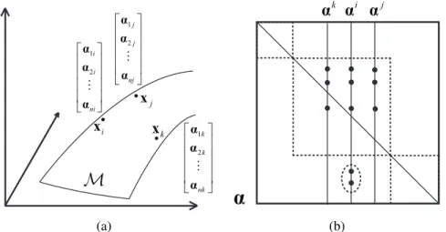
i x j x

M

1 2 i i ni             α α α M 1 2 j j nj             α α α M k x 1 2 k k nk             α α α M (a) i α αj k α

α

(b)

Figure 3.1: (a) Illustration of the manifold assumption used in our`0_-`1_-graph. This figure shows an example of a two-dimensional submanifoldMin the three-dimensional ambient space. Three neighboring pointsxi,xj andxkin the

submanifold are supposed to have similar sparse codes, i.e.

αi = [α1i, . . . ,αni]>,αj = [α1j, . . . ,αnj]>andαk = [α1k, . . . ,αnk]>,

according to the manifold assumption. `0_-distance_k_αi₋_αj_k

0is used to measure the distance between sparse codes for`0_-`1_{-graph, while}_`2_-distance kαi−αjk2 is used for most existing sparse representation methods using graph regularization. (b) Illustration of the coefficient matrixαcomprising the sparse codes of all the data, where the black dots indicate nonzero elements, and the inner dashed box specifies the scope of correct neighbors, i.e. the ones in the same ground truth cluster. xkandxj choose the correct neighbors, and the local

smoothness on the local sparse graph structure would encouragexi to abandon

the two wrong neighbors encompassed by the dashed ellipse.

High dimensional data always lie on or close to a submanifold of low intrinsic dimension, and clustering the data according to its underlying manifold structure is important and challenging in computer vision and machine learning. While `1-graph demonstrates better performance than many traditional similarity-based

(31)

clustering methods, it performs sparse representation for each datum indepen-dently without considering the geometric information and manifold structure of the entire data. On the other hand, in order to obtain the data embedding that ac-counts for the geometric information and manifold structure of the data, the mani-fold assumption [5] is usually employed [6, 7, 8, 9]. Interpreting the sparse code of a data point as its embedding, the manifold assumption in the case of sparse repre-sentation for most existing methods requires that if two pointsxiandxj are close

in the intrinsic geometry of the submanifold, their corresponding sparse codesαi

and αj are also expected to be similar to each other in the sense of `2-distance [8, 9]. In other words,αvaries smoothly along the geodesics in the intrinsic ge-ometry (see Figure 3.1(a)). Based on the spectral graph theory [39], extensive literature uses graph Laplacian to impose local smoothness of the embedding and preserve the local manifold structure [5, 8, 9]. Given a proper symmetric similar-ity matrixS, the sparse codeαthat captures the local geometric structure of the data in accordance with the manifold assumption by graph Laplacian minimizes the following`2regularization term:

1 2 n X i=1 n X j=1 Sijkαi−αjk22 = Tr(αLSα>) (3.5)

where the `2-norm is used to measure the distance between sparse codes. LS = DS−S is the graph Laplacian using the adjacency matrixS, the degree matrix DS is a diagonal matrix with each diagonal element being the sum of the ele-ments in the corresponding row ofS, namely(DS)ii=

n

P

j=1

Sij. To the best of our

knowledge, such `2 regularization is employed by most methods that use graph regularization for sparse representation. Incorporating the`2 _{regularization term}

into the optimization problem of`1_{-graph, the formulation of}_`2_graph

regulariza-tion for`1_{-graph, which is also named}_`2_-_`1_-graph_{, is}

min α L(α) = n X i=1 kxi−Xαik22+λ`1kαik₁+γ_`2Tr(αL_Sα>) (3.6) where γ_`2 > 0 is the weighting parameter for the `2 regularization term. Fol-lowing the representative `2 _{graph regularization method [8, 9],} _S _{is chosen as} the adjacency matrix of K-nearest-neighbor (KNN) graph, i.e. Sij = 1 if and

(32)

used in the manifold learning literature, such as Locally Linear Embedding [50], Laplacian Eigenmaps [51] and Sparse Manifold Clustering and Embedding [49], to establish the local neighborhood in the manifold. AlthoughSis not symmetric, letting S0 = S+S₂>, then a symmetric adjacency matrix can be used in the graph regularization term without changing its value: Tr(αLS0α>) = Tr(αL_Sα>).

In the following subsection, we propose `0_-`1_{-graph, which uses} _`0_{-norm to} measure the distance between the sparse codes in the graph regularization term in (3.6) based on the manifold assumption on the local structure of the sparse graph, leading to `0 graph regularization for `1-graph with superior clustering perfor-mance.

Algorithm 1Data Clustering by`0_-`1_-Graph

Input:

The data setX ={xi}ni=1, the number of clustersc, the parameterλ,γ,Kfor `0-`1-graph, λ`1 for the initialization of the `0-`1-graph, maximum iteration number Mc for coordinate descent, and maximum iteration number Mp for

the iterative proximal method, stopping thresholdε

1: r= 1, initialize the coefficient matrix asα(0) =α`1.

2: whiler≤Mcdo

3: Obtainα(r) _from_α(r−1)_{by coordinate descent. In}_{i-th (}₁_≤_i _≤_{n) step of} ther-th iteration of coordinate descent, solve (3.8) using the iterative prox-imal method (3.9) and (3.12) to updateαiin each iteration of the proximal method. 4: if|L(α(r))−L(α(r−1))|< εthen 5: break 6: else 7: r=r+ 1. 8: end if 9: end while

10: Obtain the sub-optimal coefficient matrixα∗ when the above iterations con-verge or maximum iteration number is achieved.

11: Build the pairwise similarity matrix by symmetrizingα∗: W∗ = |α∗|+₂|α∗|>, compute the corresponding normalized graph LaplacianL∗ = (D∗)−12(D∗− W∗)(D∗)−12, whereD∗ is a diagonal matrix withD∗

ii = n

P

j=1 W∗_ij

12: Construct the matrixv = [v1, . . . ,vc] ∈ IRn×c, where {v1, . . . ,vc} are the

ceigenvectors ofL∗ corresponding to its csmallest eigenvalues. Treat each row ofvas a data point inIRc_{, and run K-means clustering method to obtain}

the cluster labels for all the rows ofv.

Output: The cluster label ofxi is set as the cluster label of the i-th row of v,

(33)

3.3

The proposed

`

0

-

`

1

-Graph

Different from the previous graph regularized sparse representation methods [8, 9] where the sparse code of a data point serves as feature representation of that point for various learning tasks, the performance of sparse graph based clustering solely depends on the sparse graph. Since the only information of each data point in the sparse graph is its associated local structure of the sparse graph, rendering a sparse graph in accordance to the geometric information and manifold structure of the data requires the manifold assumption on the local sparse graph structure, mentioned in the introduction. This new variant of the manifold assumption en-courages local smoothness on the local sparse graph structure. Such local smooth-ness is prone to produce the sparse graph complying to the manifold structure of the data. It also encourages the data points to coordinate with each other in se-lecting their neighbors. In the frequent case that most of the neighbors of a data point have nearly correct neighbor selection, the said local smoothness effectively advises this point to make a potentially better neighbor selection, compared to choosing neighbors on its own, especially when this point is subject to noise or itself is an outlier (see Figure 3.1(b)).

To facilitate optimization in terms of the sparse codes, we restrict the informa-tion of the local sparse graph structure for a data point to be that contained in its sparse code. Based on the construction of the sparse graph in Section 3.2, the local sparse graph structure contained in the sparse code of a data point is its support and nonzero elements: the support determines the neighbors it chooses and the nonzero elements contribute to the edge weights. Note that if the sparse codes of two data points have zero `0-distance, then they have similar local sparse graph structure. This motivates us to propose `0_-`1_{-graph which employs} _`0_{-norm to} measure the distance between sparse codes and promote local smoothness of the sparse graph structure. The optimization problem of`0-`1-graph is

min α L(α) = n X i=1 kxi−Xαik22+λkαik1+γRS(α) (3.7) whereRS(α) = n P i,j=1

Sijkαi−αjk0 is the `0 regularization term, S is the adja-cency matrix of the KNN graph, γ > 0is the weighting parameter for`0 _graph regularization term.

We use coordinate descent to optimize (3.7) with respect toαi_{, i.e. in each step}

thei-th column ofα, while fixing all the other sparse codes{αj_}

(34)

of coordinate descent, the optimization problem forαi _is min αi F(α i_{) =}_k_x i−Xαik22+λkαik1+γR_S˜(αi) (3.8) whereR_S˜(αi) = n P j=1 ˜ Sijkαi−αjk0,S˜ =S+S>

Inspired by recent advances in solving non-convex optimization problems by proximal linearized method [52], we propose an iterative proximal method to op-timize the nonconvex problem (3.8). In the following text, the superscript with bracket indicates the iteration number of the proposed proximal method or the iteration number of the coordinate descent without confusion.

Int-th (t≥ 1) iteration of our proximal method, gradient descent is performed on the square loss term of (3.8), i.e.P(αi_{) =}_kx

i−Xαik22: ˜ αi(t) ₌_αi(t−1)₋ 2 τ s(X > Xαi(t−1)−X>xi) (3.9)

where τ > 1 is a constant and s is the Lipschitz constant for the gradient of functionP(·), namely

k∇P(Y)− ∇P(Z)kF ≤skY−ZkF, ∀Y,Z∈IRn (3.10)

Thenα(t)is obtained as the solution to the following`0-`1regularized problem:

αi(t) = arg min_v_∈_IRn_,_v i=0 τ s 2 kv−α˜ (t)_k2 2+λkvk1+γR_S˜(v) (3.11) Using the fact thatmax{|α˜(t)_{| −} λ

τ s,0} ◦sign( ˜α (t)₎_{is the solution to} arg min v τ s 2 kv−α˜ (t)_k2 2+λkvk1

where◦denotes element-wise multiplication, Proposition 1 below shows the closed form solution to the`0-`1regularized subproblem (3.11):

Proposition 1. DefineF(vk) = τ s₂ kvi −α˜ (t) k k22+λ|vk|+γR_S˜(vk)forvk ∈ IR andR_S˜(vk), n P j=1 ˜

Sijkvk−αjkk0. Letu= max{|α˜(t)| −_{τ s}λ,0} ◦sign( ˜α(t)), and

letv∗be the optimal solution to (3.11). Then thek-th element ofv∗is

v∗_k =    arg min_v k∈{uk}∪{αjk}{j:˜S_ij6=0}F(vk) : k 6=i 0 : k =i (3.12)

(35)

Proposition 1 suggests an efficient way of obtaining the solution to (3.11). Ac-cording to (3.12), αi(t) ₌ _v∗

can be obtained by searching over a candidate set of sizeK+ 1, whereK is the number of nearest neighbors to construct the KNN graphSfor`0_-`1_-graph.

The iterative proximal method starts from t = 1 and continues until the se-quence {F(αi(t)₎_} _{converges or maximum iteration number is achieved. When}

the proximal method converges or terminates for eachαi, the step of coordinate descent for αi is finished and the optimization algorithm proceeds to optimize other sparse codes. We initialize α as α(0) = α`1 and α_`1 is the sparse codes generated by `1-graph by solving (3.3) with some proper weighting parameter λ_`1. In all the experimental results shown in the next section, we empirically set λ`1 = 0.1.

The data clustering algorithm by`0_-`1_{-graph is described in Algorithm 1.} Let-ting the maximum iteration number for coordinate descent beMc, and maximum

iteration numberMp for each step of the coordinate descent, then the time

com-plexity of running the coordinate descent for `0-`1-graph isO(McMpn3).

More-over, the following theorem shows that with a properly chosens for gradient de-scent in (3.9), each iteration of the proposed proximal method decreases the value of the objective function F(·) in (3.8). Since each step of coordinate descent decreases the objective L, our coordinate descent method optimizing L always converges.

Theorem 3. Let s = 2σmax(X>X) where σmax(·) indicates the largest

eigen-value of a matrix, then the sequence{F(αi(t)₎_}_{generated by the proximal method}

with (3.9) and (3.12) decreases, and the following inequality holds fort≥1:

F(αi(t))≤F(αi(t−1))− (τ−1)s

2 kα

i(t)₋_αi(t−1)_k2

F (3.13)

It follows that the sequence{F(αi(t))}tconverges as a sequence indexed byt

for each 1≤i≤n, so our proximal method converges.

Table 3.1: Clustering Results on Three UCI Data Sets

Data Set Measure KM SC `1_-graph _SMCE _`2_-_`1_-graph _`0_-_`1_-graph

Heart AC 0.5889 0.6037 0.6370 0.5963 0.6259 0.6481 NMI 0.0182 0.0269 0.0529 0.0255 0.0475 0.0637 Ionosphere AC 0.7095 0.7350 0.5071 0.6809 0.7236 0.7635 NMI 0.1285 0.2155 0.1117 0.0871 0.1621 0.2355 Breast AC 0.8541 0.8822 0.9033 0.8190 0.9051 0.9051 NMI 0.4223 0.4810 0.5258 0.3995 0.5249 0.5333

(36)

Table 3.2: Clustering Results on COIL-20 Database COIL-20

# Clusters Measure KM SC `

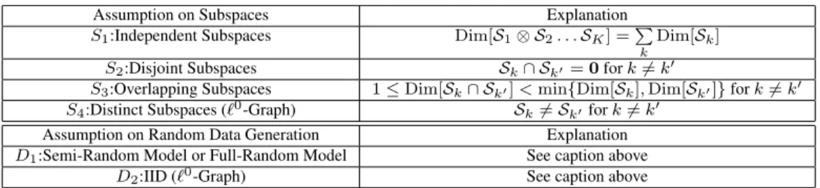
1_-graph _SMCE _`2_-_`1_-graph _`0_-_`1_-graph

K = 4 AC 0.6625 0.6701 1.0000 0.7639 0.7188 1.0000 NMI 0.5100 0.5455 1.0000 0.6741 0.6129 1.0000 K = 8 AC 0.5157 0.4514 0.7986 0.5365 0.6858 0.9705 NMI 0.5342 0.4994 0.8950 0.6786 0.6927 0.9581 K = 12 AC 0.5823 0.4954 0.7697 0.6806 0.7512 0.8333 NMI 0.6653 0.6096 0.8960 0.8066 0.7836 0.9160 K = 16 AC 0.6689 0.4401 0.8264 0.7622 0.8142 0.8750 NMI 0.7552 0.6032 0.9294 0.8730 0.8511 0.9435 K = 20 AC 0.6504 0.4271 0.7854 0.7549 0.7771 0.8208 NMI 0.7616 0.6202 0.9148 0.8754 0.8534 0.9297

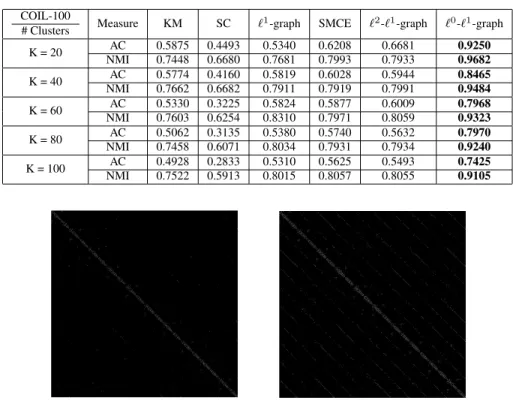
Table 3.3:Clustering Results on COIL-100 Database COIL-100

K = 20 AC 0.5875 0.4493 0.5340 0.6208 0.6681 0.9250 NMI 0.7448 0.6680 0.7681 0.7993 0.7933 0.9682 K = 40 AC 0.5774 0.4160 0.5819 0.6028 0.5944 0.8465 NMI 0.7662 0.6682 0.7911 0.7919 0.7991 0.9484 K = 60 AC 0.5330 0.3225 0.5824 0.5877 0.6009 0.7968 NMI 0.7603 0.6254 0.8310 0.7971 0.8059 0.9323 K = 80 AC 0.5062 0.3135 0.5380 0.5740 0.5632 0.7970 NMI 0.7458 0.6071 0.8034 0.7931 0.7934 0.9240 K = 100 AC 0.4928 0.2833 0.5310 0.5625 0.5493 0.7425 NMI 0.7522 0.5913 0.8015 0.8057 0.8055 0.9105

Figure 3.2: The comparison between the weighed adjacency matrixW of the sparse graph produced by`1_{-graph (right) and}_`0_-`1_{-graph (left) on the Extended} Yale Face Database B, where each white dot indicates an edge in the sparse graph.

3.4

Experimental Results

The superior clustering performance of`0_-`1_{-graph is demonstrated by extensive} experimental results on various data sets. `0_-`1_{-graph is compared to K-means} (KM), Spectral Clustering (SC), `1_{-graph, Sparse Manifold Clustering and}

(37)

Em-Table 3.4: Clustering Results on the Extended Yale Face Database B. Yale-B

c = 10 AC 0.1780 0.1937 0.7580 0.3672 0.4563 0.8750 NMI 0.0911 0.1278 0.7380 0.3264 0.4578 0.8134 c = 15 AC 0.1549 0.1748 0.7620 0.3761 0.4778 0.7754 NMI 0.1066 0.1383 0.7590 0.3593 0.5069 0.7814 c = 20 AC 0.1227 0.1490 0.7930 0.3542 0.4635 0.8376 NMI 0.0924 0.1223 0.7860 0.3789 0.5046 0.8357 c = 30 AC 0.1035 0.1225 0.8210 0.3601 0.5216 0.8475 NMI 0.1105 0.1340 0.8030 0.3947 0.5628 0.8652 c = 38 AC 0.0948 0.1060 0.7850 0.3409 0.5091 0.8500 NMI 0.1254 0.1524 0.7760 0.3909 0.5514 0.8627

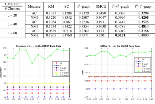
Table 3.5: Clustering Results on CMU PIE Data CMU PIE