Dimension Reduction and Classification for High Dimensional Complex Data.

(1)

ABSTRACT

ZHANG, BO. Dimension Reduction and Classication for High Dimensional Complex Data. (Under the direction of Lexin Li and Hua Zhou.)

The typical modern scientic data set has increased exponentially not only in size but also in complexity, and the diculties of eectively analyzing such data sets have multiplied. This dissertation addresses several dimension reduction and/or classication challenges posed by this new wealth of data.

First, we concentrate on the classication problem with matrix-valued predictors, and propose a novel nuclear norm penalized linear discriminant analysis (LDA), which eciently tackles the high dimensionality while preserving the matrix structure. Our pro-posal is motivated by the fact that the classical LDA can be reconstructed exactly via least squares and the matrix-valued parameters often own a low-rank structure. An eective algorithm to solve the nuclear norm minimization problem with guaranteed convergence rate is introduced. Superior performance of the proposed method is demonstrated on both synthetic and real examples.

Next, we focus on the classication problem with tensor-valued predictors, and pro-pose a tensor LogitBoost method, which organically combines the boosting algorithm and the tensor regression algorithm. The proposed method is o-the-shelf, computationally ecient and adaptable to multiple modalities of brain imaging. Experiments on two real data sets validate the performance of the proposed method.

(2)

(3)

(4)

Dimension Reduction and Classication for High Dimensional Complex Data

by Bo Zhang

A dissertation submitted to the Graduate Faculty of North Carolina State University

in partial fulllment of the requirements for the Degree of

Doctor of Philosophy

Statistics

Raleigh, North Carolina 2012

APPROVED BY:

Wenbin Lu Ana-Maria Staicu

Lexin Li

(5)

DEDICATION

(6)

BIOGRAPHY

(7)

ACKNOWLEDGEMENTS

I would like to take this opportunity to express my upmost gratitude and appreciation to my supervisors, Dr. Lexin Li and Dr. Hua Zhou for their guidance, valuable insight and support over the course of my graduate studies. Their helpful feedback on my work was greatly appreciated and I have learned a lot from them.

I would also like to thank my committee members, Dr. Wenbin Lu, Dr. Ana-Maria Staicu and Dr. Tao Pang for reviewing my dissertation and sharing their constructive suggestions.

I would like to extend my deep appreciation to the Department of Statistics at North Carolina State University for providing great academic and logistic support for my gradu-ate study. I would like to thank knowledgeable faculty members for their excellent lectures and thank friendly sta Adrian and Alison for their assistance.

(8)

LIST OF TABLES

Table 2.1 Testing error for two-dimensional low-rank shape signals . . . 25

Table 2.2 Testing error for two-dimensional high-rank shape signals . . . 25

Table 2.3 Testing error for synthetic signals with Σ = I4096 . . . 26

Table 2.4 Testing error for synthetic signals with Σ = Ω64⊗I64 . . . 27

Table 2.5 Testing error for EEG data . . . 30

Table 3.2 Training and testing subjects from dierent sites . . . 50

Table 3.3 Testing error for sMRI Data . . . 55

Table 4.1 Dimension reduction for design M1 . . . 75

Table 4.4 Dimension reduction for design G1 . . . 79

Table 4.11 Proxies information for temperature data . . . 86

(11)

LIST OF FIGURES

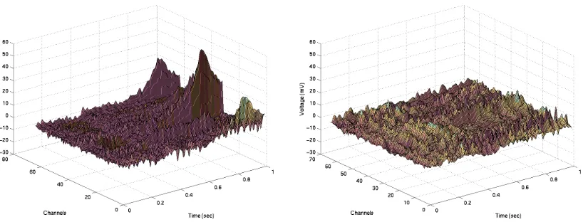
Figure 2.1 EEG patterns of an alcoholic and a control subject . . . 8

Figure 2.2 Regularized estimators of two-dimensional shape signals . . . 24

Figure 2.3 Plot of error versus regularization parameter . . . 27

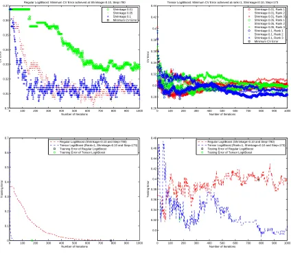
Figure 3.1 Analysis procedure for downsized sMRI data of size 25×29×25. 51

Figure 4.1 Scatter plot for the two sucient predictors for EEG data . . . . 84

(12)

Chapter 1 Introduction

Recent rapid advances in technology and instrumentation are creating high dimensional complex data sets that are not amenable to the traditional statistical analysis methods fa-miliar to statisticians. Traditional methods are often fractured and ineective not merely because of the high dimensionality of the data, but also because of the complex structure of the data. In this dissertation, we describe three innovative dimension reduction and/or classication techniques for dealing with some examples of such data sets.

There have been a signicant body of work devoted to the high dimensional classica-tion problem (Nguyen and Rocke 2002; Huang and Pan 2003; Marchette and Priebe 2003; Tzeng, Lum, and Ma 2003; Boulesteix 2004; Ruschhaupt et al. 2004; Bair et al. 2006; Zou, Hastie, and Tibshirani 2006; Tibshirani and Hastie 2007). However, recent scientic research shows that there often exist complex data which add further complications to the high dimensional classication problem.

(13)

pixels; and remote sensing data, which contain the accurate surface reectance values arranged in rows and columns of the raster; and ow cytometric data, expressed as the uorescence intensity of multiple cells at multiple channels; and Magnetoencephalography (MEG) data, which record magnetic elds over the scalp by a hundred or more sensor channels over a very short time interval.

Our motivating example is the alcoholism study using an electroencephalography (EEG) data set (http://kdd.ics.uci.edu/datasets/eeg/eeg.data.html). Each of the 122 subjects (77 subjects with alcoholism and 44 controls) was asked to look at the prepared stimuli, which were pictures of objects from the Snodgrass and Vanderwart picture set (Snodgrass and Vanderwart 1980). During one exposure interval, the

volt-age values were recorded from 64 channels of electrodes placed on the subject's scalp

at 256 time points. In other words, the sampling unit of the EEG data is a 256 by 64

random matrix. It is of great scientic interest to predict the alcoholism status based on the subject's EEG data. For this purpose, the well-known linear discriminant anal-ysis (LDA), which has demonstrated competitive performance in spite of its simplicity, oers a potentially useful mechanism. However, both the nature of the High Dimension, Low Sample Size (HDLSS) data and the presence of the matrix-valued predictors pose signicant challenges to the application of LDA. Naively attening the matrix-valued predictor into a vector and performing LDA with vectorized predictors would fail due to the singularity of the sample covariance estimate and the destruction of the inherent structural information. Consider the EEG data as an example. An EEG image of size

256 by64 implies a feature space of 256×64 = 16384 dimensions. Covariance matrices

of size 16384×16384 = 268M are almost always singular, since the sample size needs to

be at least268M for them to be non-degenerate.

(14)

sparsity on the covariance matrices so that they can be regularized (Friedman 1989; Krzanowski et al. 1995; Dudoit, Fridlyand, and Speed 2002; Bickel and Levina 2004; Xu, Brock, and Parrish 2009). However, the classier with a better estimate of the inverse covariance matrix might not perform reasonably well (Fan and Fan 2008).

Some further developments have been focusing on assuming sparsity on the mean

vector. However, such `1 penalty enforced on the LDA coecients cannot preserve the

matrix structure.

In Chapter 2, we propose a novel nuclear norm penalized LDA, which eciently com-presses the high dimensionality while maintaining the matrix structure. Our proposal is based rmly on the fact that the traditional LDA algorithm for the two-class classi-cation problem can be reconstructed exactly via least squares and the matrix-valued parameters often have, or can be well approximated by, a low-rank structure. The rank of the matrix-valued parameters in our proposed method is not xed and needs to be tuned, and thus corresponds to the soft-thresholding in the classical vector-valued pre-dictor case. Looking for the nuclear norm penalized solution is a convex optimization problem and a highly ecient estimation algorithm with guaranteed convergence rate is introduced. Synthetic and real examples show that our nuclear norm penalized LDA

outperforms the traditional `1 norm penalized LDA.

More complexity is added to the high dimensional data when the sampling unit is in the form of a higher order tensor or a multidimensional array. Examples are video clip data, which collect a set of images at multiple time points; and diusion tensor imaging (DTI) data, which quantify three-dimensional measures of water diusion; and positron emission tomography (PET) data, which represent a three-dimensional visualization of the tracer concentration within the body.

(15)

projects.nitrc.org/indi/adhd200/), in which structural magnetic resonance imaging (sMRI) data and functional magnetic resonance imaging (fMRI) data for 776 children (491 controls and 285 ADHD) were released. The sMRI data are three-dimensional tensor and the fMRI data are four-dimensional tensor including three spatial dimensions chang-ing over time. The goal of the competition is to develop novel strategies for predictchang-ing ADHD diagnostic status based on the individual's sMRI data or fMRI data. However, high dimensionality and complex structure of the MRI data inhibit the accurate classi-cation.

In Chapter 3, we propose a tensor LogitBoost method for classication, which or-ganically combines the LogitBoost algorithm (Ridgeway 1999; Friedman 2001) and the recently proposed tensor regression algorithm (Zhou, Li, and Zhu 2012). The core part is to learn the classiers by tting a weighted tensor linear regression. The basic idea behind the weighted tensor linear regression is to impose a particular low-rank structure (CANDECOMP/PARAFAC decomposition) on the tensor-valued regression parameters. Such solution ts the model at a xed rank of the tensor, and thus corresponds to the hard-thresholding in the classical vector-valued predictor case. The method is o-the-shelf", computationally eective and adaptable to various modalities of brain imaging, such as sMRI, DTI, fMRI, PET, EEG and MEG. Experiments on the EEG data set and the sMRI data set validate the performance of the proposed method.

(16)

dimension reduction (KDR; Fukumizu, Bach, and Jordan 2009), and principal support vector machine (PSVM; Li, Artemiou, and Li 2011). However, the increasing complex-ity of the data often adds further complications to the sucient dimension reduction problem.

Besides the complexity posed by the matrix-valued predictors or the tensor-valued predictors, complexity could also be present in the high dimensional data when the vector-valued predictors naturally fall into dierent groups or domains at the time of data collection. For instance, in cognitive science, a battery of cognitive measures belong to dierent cognitive domains; in computational biology, genes belong to dierent biological pathways.

Our motivating example is a temperature study (Mann et al. 2008; McShane and Wyner 2011), where 116 proxies from 6 dierent groups are collected. Those proxies are available for both historical period (999-1949) and modern instrumental period (1950-1998). The goal of this study is to construct a statistical model which relates the observed temperature anomalies to the proxy predictors for modern instrumental period, and then use this model to predict temperature anomalies for the historical period to study how temperature has changed.

Conventional dimension reduction could be applied prior to any modeling eort for such high dimensional regression. However, the fact that these 116 proxies come from 6 dierent groups provides structure information that should be considered in the dimen-sion reduction process.

(17)

(18)

Chapter 2 Low-rank Linear Discriminant Analysis

2.1 Introduction

Modern engineering and scientic applications to geography, meteorology, astronomy and medicine are often producing massive data sets for which the sampling unit is not in the form of a vector-valued object but in the form of a matrix-valued object. The row and column of the matrix-valued object represent dierent types of information. Representative data include:

two-dimensional digital image data, which consist of the brightness values ranging from 0 (black) to 255 (white) at a xed number of rows and columns of pixels;

remote sensing data, which contain the accurate surface reectance values arranged in rows and columns of the raster;

(19)

EEG data, which measure the voltage values from multiple electrodes placed on the scalp over a short period of time;

MEG data, which record magnetic elds over the scalp by a hundred or more sensor channels over a very short time interval.

Classication based on such data plays a very important role in these applications but confronts the researchers with various challenges. For instance, Figure 2.1 exhibits characteristic EEG patterns of an alcoholic subject (left panel) and a control subject (right panel). The vertical axis denotes the voltage value and two horizontal axes rep-resent channel and time. It is highly suggested that the EEG patterns are signicantly dierent between these two groups and hence it is of great scientic interest to perform the classication of the alcoholics and non-alcoholics via the EEG data.

(20)

2.1.1 Literature Review

Image classication is the problem of predicting the class label of a new unlabeled image, on the basis of a training sample of images whose class labels are known. A short survey about image classication methods used in two important applications is presented as follows.

Remote Sensing Data

Remote sensing has been be used in several dierent areas, including geography, mete-orology and land-cover mapping. For example, it is of considerable practical interest to retrieve roads, forests and rivers from remote sensing data and to update an existing transportation system. However, classication of remote sensing data is a complex and challenging task, which can be jeopardized by a number of factors, such as the specic need of the user, the technical skills of the analyst, the size of the target area and the economic condition.

Dierent features in a remote sensing image have dierent capabilities of extracting a specic land-cover class. Classication using all the features may decrease the classi-cation accuracy (Price, Guo, and Stiles 2002). Hence, selecting the right set of features is extremely important for separating land-cover classes. A number of classical feature selection methods have been applied to reduce the amount of redundancy in remote sensing data, such as principal component analysis (PCA; Linders 2000), wavelet trans-form (Myint 2001) and spectral mixture analysis (SMA; Okin et al. 2001; Asner and Heidebrecht 2002; Lobell et al. 2002).

(21)

and Taberner 2004), decision tree (Pal and Mather 2003; Lawrence et al. 2004), and knowledge-based classication (Thomas, Hendrix, and Congalton 2003; Schmidt et al. 2004), can be an advantageous alternative to the popular parametric classiers as they are eective to handle either single- or multi-source remote sensing data.

Two-dimensional Brain Image Data

MEG can measure the magnetic elds of the currents, which are produced by the electrical activity of active neurons of the brain. Such current can also reach the scalp surface and result voltage dierences on the scalp, which can be recorded as EEG.

One advantage of EEG and MEG over the other brain image data is their extremely high temporal resolution and can therefore detect more subtle neuronal events. The other advantage of EEG and MEG is that they are matrix-valued. Each row represents time and each column represents variation in the electric potentials (EEG) or magnetic elds (MEG) originating from cortical neurons.

(22)

with an overall classication accuracy varied from 62.5% to79.17%.

2.1.2 Motivation

(23)

Cai, Zhang, and Zhou 2010). However, the LDA classier with a better estimate of the inverse covariance matrix might not be better than random guessing if all the features are used (Fan and Fan 2008).

A particular focus of some further developments or modications in this vein has been the eective selection of the features. Tibshirani et al. (2002) proposed the nearest shrunken centroids (NSC) classier, which can be treated as a heavily restricted version of LDA. They assumed a diagonal within-class covariance matrix and utilized the shrunken centroids rather than the simple centroids as a feature for each class. Fan and Fan (2008) then proposed the features annealed independence rule (FAIR), under which a subset of important features can be selected by hard-thresholding marginal t-statistics.

While assuming the sparsity on the covariance matrix has been quite useful, it is not without drawbacks. In particular, correlations among the predictors for the high dimen-sional data are ignored and could therefore lead to the inferior classication. The other vein is to assume sparsity on the LDA coecients. Mai, Zou, and Yuan (2012) proposed a procedure for sparse LDA and the sparsity was assumed on the mean vector not on the covariance matrix. Their method can consistently estimate the Bayes classication direction.

(24)

vectorized image signal would not benet from the wealth of structural information. In other words, the sparse LDA is ineective for the two-dimensional image data.

In this chapter, we concentrate on the two-dimensional brain image classication and propose a novel nuclear norm penalized version of LDA, called low-rank LDA. The proposed method successfully tackles the high dimensionality of the involved image data while maintaining the matrix structure. Our proposal is original and is partly motivated by the fact that the classical LDA direction can be derived perfectly via least squares. Penalizing the nuclear norm of the image signal can circumvent the singularity of the covariance matrix, enforce the low-rank structure and allow for better interpretation of the LDA coecients.

The proposed method performs naturally for high dimensional classication with matrix-valued predictors. As we have mentioned earlier, when facing with high dimen-sional image data, existing solutions often need a classical feature extraction/selection step followed by a rened classication, or a rened feature extraction/selection step prior to a traditional classication. In contrast, our proposed classication procedure combines these two tasks in a unied framework.

The extensive simulation studies and real data analysis validate the performance of the proposed method.

2.1.3 Outline

(25)

investigate the empirical performance of the proposed method, and to compare with sparse LDA solutions. In Section 2.4, low-rank LDA is applied to the motivating EEG data for further illustration. We conclude the chapter in Section 2.5 with a brief discussion on future directions.

2.2 Method

2.2.1 Notation

All vectors are written as boldface lowercase and matrices are written as boldface

up-percase. Given a vector β ∈ _Rp, we consider the _`

1 norm ||β||1, that is, the sum of the

absolute value of the coordinates of β.

Given a matrix B∈_Rpl×pr, we consider the Schatten-_p norm

||B||Sp =

 

min(pl,pr)

X

j=1

σp_j(B)

 

1/p

,

where p∈(0,∞) is xed and σj(B)is the j-th singular value of the matrix B.

A widely used Schatten-p norm is the Schatten-1 norm:

||B||∗ =

X

j

σj(B).

The Schatten-1 norm is also called nuclear norm or trace norm. Without ambiguity, we

(26)

For the consistency, the Schatten-0norm of the matrix B is dened as

||B||S0 =

 

min(pl,pr)

X

j=1

σ0_j(B)

 .

Under such denition, the Schatten-0 norm of the matrix B is exactly the rank of B,

i.e., ||B||S0 =rank(B).

Given two matricesA= [a1. . .an]∈Rm×nandC = [c1. . .cq]∈Rp×q, the Kronecker

product ofA and C is the mp-by-nq matrix

A⊗C =

     

a11C · · · a1nC

... ...

am1C · · · amnC

      .

If m=p and n=q, the inner product of Aand C is dened as

hA,Ci=hvecA,vecCi=X

i,j

aijcij,

where vec is the vectorization operator that stacks the columns of a matrix below one

another into a vector.

2.2.2 LDA as Least Squares Regression

Consider a two-class classication problem where x ∈ _Rp _{denotes the vector-valued}

predictor and G= 1,2 represents the class label. The underlying assumption of LDA is

(27)

where g ∈ {1,2}. In other words, the predictors from class 1 and class 2 come from two dierent normal distributions, each with distinct mean vectors but same covariance matrix.

Let π1 and π2 be the prior probability of class 1 and class 2, respectively, with

π1 + π2 = 1. If a new data point xnew is observed, then the LDA classication rule,

which can minimize the within-class distance and maximize the between-class distance

simultaneously, is to assign x_new to class2 if

{x_new−1

2(µ1 +µ2)}

T_Σ−1₍_µ

2−µ1) + log

π2

π1

>0

and class 1 otherwise.

In practice, the true values of µ1 and µ2 are unknown and can be estimated by

ˆ

µ1 =

1 n1

X

gi=1

xi,

and

ˆ

µ2 =

1 n2

X

gi=2

xi,

where n1 and n2 are sample sizes within class 1 and class 2, respectively. Also, the true

value of Σ is unknown and can be estimated by

ˆ

Σ = 1

n1+n2−2

[X

gi=1

(xi−µˆ1)(xi−µˆ1)T+

X

gi=2

(xi−µˆ2)(xi−µˆ2)T].

(28)

only if

{x_new− 1

2( ˆµ1+ ˆµ2)}

T_Σˆ−1_{( ˆ}_µ

2−µˆ1) + log

n2

n1

>0. (2.1)

If the class labels for the two classes are coded as

y=

    

− n

n1

if G= 1,

n n2

if G= 2,

where n=n1+n2, a corresponding least squares problem then can be formulated as

( ˆβ₀ls,βˆls) = argmin

β0,β

n

X

i=1

(yi−β0 −xTiβ)

2_. _(2.2)

The solution βls is given by

ˆ

βls= ˆΣ−1( ˆµ2−µˆ1),

up to some positive constant. Hence, the coecient vector derived from least squares,_βˆls_,

is equivalent to the LDA direction given in (2.1), up to a scalar multiple (Fisher 1936; Ripley et al. 1996). This correspondence holds for any distinct coding of the class labels (Hastie et al. 2005).

2.2.3 Low-rank LDA

Now suppose the predictor X is a pl×pr random matrix and assume

(29)

One traditional way to handle the matrix-valued predictor is to concatenate all the columns of the matrix into a column vector. However, the classical LDA with the vec-torized predictors will break down and lose the connection with least squares in cases such as this due to the following three reasons: (1) the maximum likelihood estimate of

the covariance matrix Σ in (2.1) is not invertible and the solution in (2.2) is not unique

sincen is less thanplpr; (2) collapsing the matrix-valued predictor destroys the wealth of

intrinsic structural information possessed in the image data; (3) the resulting LDA classi-er is not easy to be intclassi-erpreted, since the classication rule uses the linear combination of all the features in the image data.

To overcome these issues, we propose to regularize LDA further via penalized least squares regression. For the matrix-valued data, the true signal often has, or can be well approximated by, a low-rank structure. Hence, a natural idea is to approximate the LDA coecients using a low-rank matrix by minimizing

1 n

n

X

i=1

(yi−β0− hB,Xii)2+λ||B||S0, (2.3)

where λ is the positive regularization parameter. However, the minimization problem

in (2.3) is dicult to solve since the rank minimization is known as non-deterministic polynomial-time hard (NP-hard). To overcome this problem, we propose to solve the

Schatten-pnorm penalized least squares problem by minimizing

1 n

n

X

i=1

(yi−β0− hB,Xii)2+λ||B||pSp, (2.4)

where 0< p < ∞.

(30)

of (2.3) than the one under p ≥ 1. Also, similar to the `p norm in vector estimation

problems, the Schatten-p norm is non-convex under 0< p <1.

While a number of algorithms have been proposed to address this Schatten-p norm

(0< p <1) penalized problem (Argyriou, Evgeniou, and Pontil 2008; Mohan and Fazel

2010; Argyriou, Micchelli, and Pontil 2010), how to nd a global minimum in (2.4) is

still an open question. The nuclear norm, or Schatten-1 norm, however, is a commonly

used convex relaxation of the rank function, since it is the convex envelope of the rank function over the unit ball of spectral norm (Fazel 2002). Hence, in this chapter, we focus on the following nuclear norm penalized least squares problem:

( ˆβ₀lr,Bˆlr) = argmin

β0,B

{1

n

X

i=1

(yi−β0− hB,Xii)2+λ||B||∗}. (2.5)

The resulting estimate of the coecient vector_Bˆlr _{in (2.5) will be the low-rank linear}

discriminant direction based on the correspondence between LDA and classication by

least squares. The low-rank LDA classier assigns a new observation X_new to class 2 if

and only if

˜

β₀lr +hBˆlr,X_newi>0. (2.6)

Note that_β˜lr

0 in (2.6) diers fromβˆ0lr in (2.5) unlessn1 =n2 and hence selecting the right

intercept plays a crucial role for low-rank LDA.

Mai, Zou, and Yuan (2012) presented a closed form formula for computing the optimal intercept for the linear discriminant function, which is introduced as follows:

Proposition 2 of Mai, Zou, and Yuan (2012): Suppose that a linear classier

(31)

intercept is

β₀opt =−1

2(µ1 +µ2)

T_β˜_{+ ˜}_βT_Σ_β˜_{₍_µ

2−µ1)Tβ˜}−1log

π2

π1

,

which can be estimated by

ˆ

β₀opt =−1

2( ˆµ1+ ˆµ2)

T_β˜_{+ ˜}_βT_Σ_ˆ_β˜_{_{( ˆ}_µ

2−µˆ1)Tβ˜}−1log

n2

n1

.

This proposition provides a useful tool to select the intercept for the low-rank linear discriminant function. More concretely, the intercept can be estimated by

˜

β₀lr = −1

2(vec ˆµ1+ vec ˆµ2)

T_{vec ˆ}_Blr₊

(vec ˆBlr)TΣˆ(vec ˆBlr){(vec ˆµ2−vec ˆµ1)T(vec ˆBlr)}−1log

n2

n1

.

2.2.4 Estimation Algorithm

Although the non-convexity of the minimization problem is relaxed when p = 1, the

nuclear norm term in (2.5) is still non-smooth.

A number of algorithms have been developed recently (Rennie and Srebro 2005; Weimer, Karatzoglou, and Smola 2008; Ma, Goldfarb, and Chen 2011) by employing some type of approximation to handle the non-smooth term. However, a fast global con-vergence rate for these algorithms is hard to guarantee.

(32)

problems can be adapted to solve the nuclear norm regularized non-smooth problems and

achieve the same optimal convergence rate of O(1/k2₎_{, where} _k _{is the iteration counter.}

For the k-th iteration of their algorithm, the following two steps are involved.

1. Predicting a search point S by a linear extrapolation from previous two iterates:

S(k)←B(k)+ (α

(k−1)₋₁

α(k) )(B (k)₋

B(k−1)).

Here, α(k) _{is a scalar sequence, which can be updated as}

α(k+1)←(1 +

q

1 + (2α(k)₎2_)/2.

Note that this extrapolation step makes this method dier from the traditional gradient method and improves the convergence rate signicantly.

2. Performing gradient descent from the search point S with Armijo type line search

(Nocedal and Wright 2006).

The nal remark is that ve-fold cross-validation is employed for tuning the

regular-ization parameterλ.

2.3 Simulations

(33)

to the following `1 norm penalized least squares problem,

( ˜β₀sp,Bˆsp) = argmin

β0,B

{1

n

X

i=1

(yi−β0− hB,Xii)

2

+λ||vecB||1}.

We randomly generated n two-class labels such that π1 =π2 = 0.5. Conditioning on

the class labels G(G = 1,2), we generated the pl×pr matrix-valued predictor X. More

specically, the vectorized X was generated from a normal distribution with mean µg

and covariance Σ, i.e.,

vecX|G=g ∼Nplpr(vecµg,Σ).

We set pl =pr = 64 and n = 500. Two choices of the covariance matrix Σwere I4096

and Ω64⊗I64, where Ωii = 1,Ωij = 0.6, i = 1, . . . ,64, j = 1, . . . ,64 and i 6=j. We also

setvecµ1 =0 and vecµ2 = 0.2vecB without loss of generality.

A ve-fold cross validation was employed for tuning the regularization parameter

λ. Also, a testing data set of sample size 500 was generated to evaluate the prediction

accuracy of the classication.

Two dierent types of true image signals were considered. First, a number of dierent geometric and natural shapes were examined. Second, some synthetic data with various ranks and sparsity were generated.

2.3.1 Two-dimensional Shapes

In this study, we chose the true matrix signalB as the two-dimensional shape signal. We

(34)

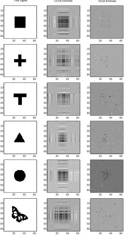
The true and estimated signals of square, cross, T-shape, triangle, disk and buttery are shown in Figure 2.2. The true signals of the upper three shapes have a low-rank structure. The true signals of the lower three shapes can be well approximated by a low-rank structure.

It is strongly suggested that the nuclear norm regularized estimator performs better

than the`1 norm regularized estimator for all the types of two-dimensional shape signals.

One might argue that some true signals are not well recovered by the nuclear norm regularized estimators. However, our goal is to recover the discriminative set, not the signal set.

Table 2.1 shows the prediction accuracy results using the two-dimensional low-rank shape signals as the true matrix signals and Table 2.2 shows the prediction accuracy results using the high-rank shape signals. Results are averaged over 100 replications. The numbers in parentheses are standard errors. The best results are highlighted in boldface. We have the following three observations. First, the low-rank LDA classier is superior to the sparse LDA classier for all two-dimensional shape signals. Second, for the true signals which don't have exact low-rank structure, the low-rank LDA classier still performs reasonably well. Third, the low-rank LDA classier performs slightly better for the cases

of correlated features, corresponding to Σ = Ω64 ⊗I64. In contrast, the sparse LDA

classier performs slightly better for the cases of uncorrelated features, corresponding to

I4096.

2.3.2 Synthetic Data

In this study, we chose the true matrix signal as the synthetic signal, which is generated

(35)

True Signal

20 40 60

10 20 30 40 50 60

LrLDA Estimate

20 40 60

10 20 30 40 50 60

SLDA Estimate

20 40 60

10 20 30 40 50 60 True Signal

20 40 60

10 20 30 40 50 60

Matrix Lasso Estimate Testing Error = 0.140

20 40 60

10 20 30 40 50 60 Lasso Estimate Testing Error = 0.490

20 40 60

10 20 30 40 50 60 True Signal

20 40 60

10 20 30 40 50 60

20 40 60

10 20 30 40 50 60 True Signal

20 40 60

10 20 30 40 50 60

Matrix Lasso Estimate Testing Error =0.21

20 40 60

10 20 30 40 50 60 Lasso Estimate Testing Error =0.430

20 40 60

10 20 30 40 50 60 True Signal

20 40 60

10 20 30 40 50 60

20 40 60

10 20 30 40 50 60 True Signal

20 40 60

10 20 30 40 50 60

20 40 60

10 20 30 40 50 60

(36)

Table 2.1: Testing error for two-dimensional low-rank shape signals

Σ Method Rectangle Cross T-shape

I4096 LrLDA 0.024 (0.010) 0.130 (0.023) 0.102 (0.023)

SLDA 0.269 (0.044) 0.350 (0.046) 0.338 (0.042)

Ω64⊗I64 LrLDA 0.017 (0.009) 0.109 (0.029) 0.087 (0.024)

SLDA 0.309 (0.044) 0.357 (0.045) 0.346 (0.042)

Table 2.2: Testing error for two-dimensional high-rank shape signals

Σ Method Triangle Disk Buttery

I4096 LrLDA 0.133 (0.026) 0.041 (0.014) 0.097 (0.022)

SLDA 0.353 (0.047) 0.283 (0.047) 0.284 (0.049)

Ω64⊗I64 LrLDA 0.130 (0.028) 0.033 (0.016) 0.088 (0.028)

SLDA 0.377 (0.046) 0.322 (0.051) 0.293 (0.040)

the rank of the generated signal eectively. The levels of the variable R are 1, 5,10 and

20. Each entry of B is a Bernoulli random variable taking value one with probability

[1−(1−s)1/R_]1/2 and hence the sparsity size can be precisely controlled by the variable

s. We varied the sparsity size s= 0.01,0.05, 0.10and 0.20. For example, s= 0.01means

about 99% of entries of B are zeros and the rest are ones.

(37)

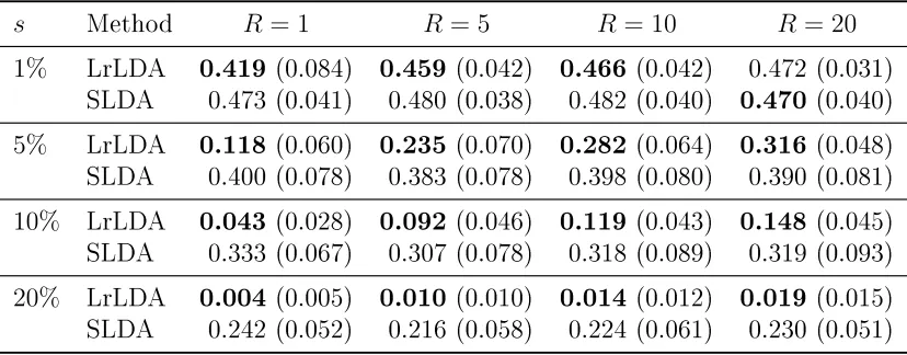
Second, as for the eects of the signal sparsity, both the low-rank LDA classier and the sparse LDA classier perform better when the signal is less sparse, which corresponds to the case that the discriminative set is easier to be identied. Third, as for the eects of the signal rank, the low-rank LDA classier preforms better when the rank is smaller and the sparse LDA is not sensitive to the rank.

Table 2.3: Testing error for synthetic signals with Σ =I4096

s Method R = 1 R= 5 R= 10 R= 20

1% LrLDA 0.419 (0.084) 0.459 (0.042) 0.466 (0.042) 0.472 (0.031)

SLDA 0.473 (0.041) 0.480 (0.038) 0.482 (0.040) 0.470 (0.040)

5% LrLDA 0.118 (0.060) 0.235 (0.070) 0.282 (0.064) 0.316 (0.048)

SLDA 0.400 (0.078) 0.383 (0.078) 0.398 (0.080) 0.390 (0.081)

10% LrLDA 0.043 (0.028) 0.092 (0.046) 0.119 (0.043) 0.148 (0.045)

SLDA 0.333 (0.067) 0.307 (0.078) 0.318 (0.089) 0.319 (0.093)

20% LrLDA 0.004 (0.005) 0.010 (0.010) 0.014 (0.012) 0.019 (0.015)

SLDA 0.242 (0.052) 0.216 (0.058) 0.224 (0.061) 0.230 (0.051)

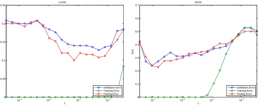
Recall that we used a ve-fold cross-validation to tune the regularization parameter

λ and Figure 2.3 shows the trace plot of the validation error, training error and testing

error versus the tuning parameterλfor low-rank LDA (left panel) and sparse LDA (right

panel), under a typical case of sparsity = 10% and rank = 10. From this trace plot, we

(38)

Table 2.4: Testing error for synthetic signals with Σ = Ω64⊗I64

s Method R = 1 R= 5 R= 10 R= 20

1% LrLDA 0.433 (0.074) 0.463 (0.038) 0.466 (0.036) 0.468 (0.035)

SLDA 0.472 (0.042) 0.470 (0.044) 0.462 (0.044) 0.459 (0.045)

5% LrLDA 0.107 (0.061) 0.204 (0.081) 0.271 (0.069) 0.312 (0.053)

SLDA 0.399 (0.075) 0.378 (0.082) 0.392 (0.085) 0.365 (0.089)

10% LrLDA 0.029 (0.019) 0.061 (0.040) 0.092 (0.041) 0.133 (0.049)

SLDA 0.335 (0.068) 0.310 (0.092) 0.322 (0.094) 0.298 (0.104)

20% LrLDA 0.007 (0.006) 0.008 (0.007) 0.010 (0.011) 0.020 (0.015)

SLDA 0.280 (0.044) 0.257 (0.073) 0.267 (0.088) 0.270 (0.094)

10−4 10−3 10−2 10−1 0 0.05 0.1 0.15 0.2 0.25 λ Error LrLDA Validation Error Training Error Testing Error 10−4 10−3 10−2 10−1 0 0.1 0.2 0.3 0.4 0.5 0.6 0.7 λ Erro SLDA Validation Error Training Error Testing Error

(39)

2.4 EEG Data Analysis

2.4.1 Data Description

EEG can measure the variations in the electric potentials, resulted from ionic current ows within the brain neurons. One advantage of EEG over the other brain image data is its extremely high temporal resolution and can therefore detect more subtle neuronal events. Hence, EEG has been widely used by neuroscientists for both clinical and research purposes.

In one EEG image data, pl electrodes are placed on the subject's scalp and voltage

values are recorded at pr time points. Therefore, the sampling unit for each subject is a

pl×pr random matrix.

We consider the motivating EEG data from an alcoholism study (http://kdd.ics. uci.edu/databases/eeg/eeg.data.html). There are two groups of subjects: an

alco-holic group of 77 subjects and a non-alcoholic group of 45 subjects. Each subject was

asked to look at the prepared stimuli, which were pictures of objects from the Snodgrass and Vanderwart picture set (Snodgrass and Vanderwart 1980). During one exposure

in-terval, the voltage values were recorded from64channels of electrodes at256time points.

The 64 electrodes are placed at dierent locations on the subject's scalp. Each subject

had120trials under three conditions: single picture, two identical pictures and two

dier-ent pictures. It is of great interest to predict the alcoholism status based on one subject's EEG image data.

In our experiment, we included only the single stimulus condition (single picture). For

each subject, we took the average of all 120 trials under the single stimulus condition,

(40)

the mean voltage value of subject i at a combination of a time point and a channel,

averaged over all 120 trials under the single stimulus condition, andYi is a binary variable

indicating whether theith subject is alcoholic (Yi = 1) or nonalcoholic (Yi = 0).

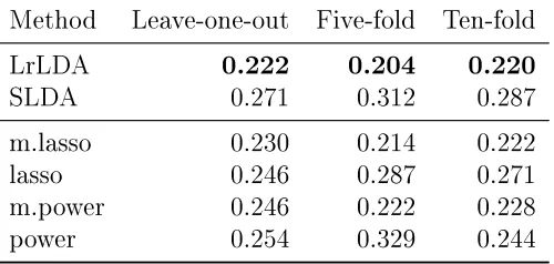
We applied low-rank LDA and sparse LDA to this EEG image data, and evalu-ated each solution via cross-validation based misclassication error. More specically,

we divided the full data into a training sample and a testing sample using k-fold

cross-validation. When k equals to the sample size, it is same as the leave-one-out

cross-validation.

For the training sample, we further employed a ve-fold cross-validation to tune the

regularization parameter λ. We then applied the tuned model which is fully based on the

training sample to the testing sample and evaluated the misclassication error rate. Zhou and Li (2012) analyzed the same data set using four methods: a matrix logistic regression with nuclear norm regularization (m.lasso), a usual vector logistic regression after vectorizing the matrix-valued predictor with a lasso penalty (lasso), a matrix logis-tic regression with power spectral regularization (m.power), and a usual vector logislogis-tic regression with a power penalty (power).

(41)

Table 2.5: Testing error for EEG data

Method Leave-one-out Five-fold Ten-fold

LrLDA 0.222 0.204 0.220

SLDA 0.271 0.312 0.287

m.lasso 0.230 0.214 0.222

lasso 0.246 0.287 0.271

m.power 0.246 0.222 0.228

power 0.254 0.329 0.244

2.5 Discussions

LDA is a well-known and commonly-used method for classication. However, it will break down if the number of the features is larger than the number of the observations, or if the predictor of interest is matrix-valued. In this chapter, we address both settings and propose an approach for extending LDA to the high dimensional matrix-valued

setting in such a way that LDA has been recast as a Schatten-p norm regularized least

squares problem. Since the minimization problem can be relaxed to the convex problem

by using the Schatten-1norm, we can consequently make use of the algorithms for convex

optimization.

It is a fact that the the smaller value of p in the Schatten-p norm corresponds to

a better approximation to the low-rank problem (the Schatten-0 norm is exactly the

rank). However, our nal goal is not to recover the low-rank structure, but to capture

the discriminant set. From this perspective, we might consider other convex Schatten-p

norms, such as Schatten-2 norm, in the future studies.

(42)

with J −1dimensions for multi-class problems, where J is the number of classes in the

training data set. Hence, it is of great interest to obtain a similar relationship between LDA and classication using least squares in multi-class cases. The current results are subject to restrictive conditions (Hastie et al. 2005) and hence the problem of nding a general theoretical link between LDA and least squares is still open.

Moreover, we restrict our studies on problems with matrix-valued predictors. In appli-cations such as structural magnetic resonance imaging (sMRI), diusion tensor imaging (DTI), positron emission tomography (PET) and functional magnetic resonance imaging (fMRI), the sampling unit is in the form of a tensor or a multidimensional array. It is natural to extend the work in this chapter to regularized least squares for tensor-valued predictors. However, the formulation of this problem requires an appropriate norm for tensors, which is in analogous to the nuclear norm for matrices.

One strategy to extend the nuclear norm regularization to tensor-valued predictors is

present as follows. If we assume that the mode-d matricization of the tensorBof interest

has a low-rank structure, the regularized tensor classication problem can be converted into a matrix classication problem by minimizing

1 λn

n

X

i=1

(yi−β0− hB,xii)2+||B(d)||pSp. (2.7)

Note that the regularization parameter λ is moved from the numerator of the

regular-ization term in Equation (2.4) to the denominator of the squared loss term in Equation

(2.7). If the rank of B(d) is small or moderate, when we can estimate the mode-d

matri-cization ofB perfectly, we can also recover the whole Bperfectly, including the ranks of

the unused modes during the estimation (Candès and Recht 2009).

(43)

the tensor. If a mode with a large rank is chosen, even if other modes with smaller ranks

exist, the wholeB cannot be recovered from a small sample size. How to choose a single

(44)

Chapter 3 Tensor LogitBoost

3.1 Introduction

More complexity is added to the high dimensional data when the sampling unit is in the form of a tensor. In this chapter, we concentrate on the classication techniques in dealing with such data, especially the brain image data.

(45)

3.1.1 Literature Review

Brain image classication methods generally comprise of three components: feature ex-traction, feature selection/dimension reduction and feature-based classication. Scientists from computer science, neuropsychiatry and other elds dene dierent types of eective features and exact the corresponding features from the original brain image data. Once the features have been dened and extracted, feature selection/dimension reduction and feature-based classication can be implemented in a statistical way.

Brain image data have been widely used for classifying the cognitive state of a human subject (Wilson and Fisher 1995; Mitchell et al. 2003; Wang, Hutchinson, and Mitchell 2003; Mitchell et al. 2004; Shirer et al. 2012). In this chapter, however, we mainly focus on the problem of classifying the disease diagnosis based on the brain image data. We now review how brain image data can be utilized to predict two important illnesses.

Schizophrenia

Schizophrenia is a complex mental disease that involves functional aection for various aspects. It has continually challenged both scientists and clinicians in terms of diagnosis, treatment and etiology. Patients with schizophrenia tend to show thought disorders,

disor-ganized speech, delusions and hallucinations. Approximately1.1%of the general

popula-tion over the age of18 has schizophrenia (http://www.nimh.nih.gov/health/topics/

schizophrenia/index.shtml). This means that Raleigh, which serves more than four hundred thousand people, might have over two thousand individuals diagnosed with schizophrenia.

(46)

The sMRI scans, for instance, could provide detailed information on which brain regions show reduction in gray matter in schizophrenia. Pardo et al. (2006) applied LDA with the 22 neuropsychological (NP) test scores and 23 quantitative sMRI measurements to classify subjects into patients with schizophrenia, patients with bipolar disorder and healthy controls. Prior to LDA, multiple regression analyses were conducted to select

eective features. The prediction accuracy of 96.4% was reported using a leave-one-out

cross-validation on the 28 subjects (10 patients with schizophrenia, 10 patients with bipolar and 8 healthy controls).

Advances in fMRI technology have also made it realistic to examine the intercon-nected neural networks, which are related to schizophrenia. Calhoun et al. (2008) applied Euclidean distance on the combination of default mode and temporal lobe components based on the fMRI to classify subjects into patients with schizophrenia, patients with bipolar and healthy controls. Both default mode and temporal lobe were identied using independent component analysis (ICA) and then merged into a single image. A dimen-sion reduction method was also employed to decrease the number of voxels. 21 patients with schizophrenia, 14 patients with bipolar and 26 healthy controls were analyzed. One randomly selected subject in each group was removed from the whole data set for

vali-dation. The rest were treated as the training sample. An average sensitivity of 90% and

specicity of 95% were reported.

(47)

the selected features and obtained a 83% leave-one-out cross-validation accuracy, which

is higher than the result of using the fMRI activation maps alone.

DTI, which is a relatively new imaging technique, can be used to visualize and mea-sure the diusion of water in brain tissue. It is especially useful for examining white matter abnormalities in the brain. As such, DTI allows for further evaluating of abnor-mal functional connectivity. Wang and Verma (2008) analyzed a data set comprising of 34 patients with schizophrenia and 36 healthy controls. They rst extracted kernel principal component analysis (KPCA) features from each of the local regions in the DTI data. This step removed the nonlinear correlation among features and reduced the dimensionality of the features. Then they adopted either a probabilistic k-NN classier or a support vector machine (SVM) to preform the classicaiton. Misclassication error of ten-fold

cross-validation ranged from 17.81% to19.68%.

Alzheimer's Disease

Alzheimer's disease (AD) is a common progressive neurodegenerative disorder among older people. It is associated with gradual memory loss and disruption of neuronal function. AD is becoming a major public health issue due to aging of the population

and about 13% of the general population over the age of 65 has Alzheimer's disease

(48)

classication tool. Almost 100% classication accuracy was achieved using a

leave-one-out cross-validation. Wang et al. (2004) noticed that the voxel values in the transformed one-dimensional domain can be viewed as a time series since they are arranged in a certain spatial order. They proposed to apply an existing time series feature extraction technique (Euclidean distance) and an existing time series dimension reduction technique (SVD) for further classication purpose. The same data set as in Kontos et al. (2004) was reanalyzed. Experimental results show that the overall prediction accuracy is above

90%.

Structural brain imaging is also a practical and valuable tool to predict AD. Mesrob et al. (2012) proposed a highly automated approach to classify patients with AD and elderly control subjects based on DTI data and sMRI data. A novel multi-modal mea-sure, which combines anatomical and diusivity measures at the voxel level, is proposed. They divided the whole-brain into 73 anatomical regions. Multi-modal characteristics were exacted in these regions. Discriminative features were selected via dierent feature selection methods. SVM was then applied for classication. 15 patients with AD and 16 elderly controls were discriminated using mean diusivity alone, combination of mean diusivity and fractional anisotropy, and multi-modal measures in the 73 regions. The

overall accuracy obtained was 65.2%, 68.6% and 72%, respectively. If relevant regions

were identied in the multi-modal measures, the overall accuracy reached 99%.

(49)

PET data, random subspace analysis was applied to train the ensembles. Results showed

an improvement of 10%−20% using this approach, compared to the classication

per-formance using each individual data source alone.

3.1.2 Motivation

Although these methods have been widely used in practice, a feature selection step needs to be conducted rst. Combining the feature selection and feature-based classication in a unied framework could avoid the step of selecting the right set of features.

In this chapter, we propose a tensor LogitBoost method, which organically combines two methods. The rst one is boosting, which was called the best o-the-shelf classier in the world by Breiman (1998). The second one is the recently proposed tensor regression method (Zhou, Li, and Zhu 2012), which handles the tensor-valued data eciently in the regression framework. One advantage of the tensor LogitBoost method lies in its ability to keep the tensor structure during the classication stage. Also, respecting tensor structure in the tensor regression step, tensor LogitBoost improves the performance of regular LogitBoost. It is o-the-shelf" and thus applies to various modalities of image data, which are all in the form of matrix or tensor. Also, it is computationally simple due to an ecient estimation algorithm for the tensor regression. The proposed method is applied to the EEG data set in Chapter 2 and a sMRI data set. Results show superior classication performance.

3.1.3 Outline

(50)

present our new method of tensor LogitBoost in detail. Tensor PCA and tuning strategy for tensor boosting are also discussed in this section. In Section 3.3 and Section 3.4, tensor LogitBoost is applied to the analysis of the EEG data and sMRI data example for further illustration. We conclude the chapter in Section 3.5 with a discussion on future extensions.

3.2 Method

3.2.1 Notation

Given two matrices A = [a1. . .an] ∈ Rm×n and B = [b1. . .bq] ∈ Rp×q, if A and B

have the same number of columns n=q, then the Khatri-Rao product is dened as the

mp×n columnwise Kronecker product

AB= [a1⊗b1 . . . an⊗bn].

See Section 2.2.1 for the denition of Kronecker product.

The mode-d matricization, B(d) ∈Rpd×

Q

d06=dpd0, is a matrix with columns the mode-_d

bers of B. More precisely, the (i1, . . . , iD) element of the tensor B maps to the (id, j)

element of the matrix B(d), wherej = 1 +P_d0₆₌_d(id0 −1)Q

d00_<d0_,d00₆₌_dpd00.With d= 1, we

observe thatvecBis the same as vectorizing the mode-1 matricizationB(1). The mode-d

multiplication of the tensor B with a matrix U ∈ _Rpd×q multiplies the mode-_d bers of

X by U, yielding B×dU ∈ Rp1×···×q×···×pD. In other words, mode-d matricization of

B×dU is U X(d).

An outer product ofDvectorsbd ∈Rpd,d= 1, . . . , D,b1◦b2◦· · ·◦bD is ap1×· · ·×pD

(51)

We say a tensor B∈ _Rp1×···×pD admits a CANDECOMP/PARAFAC decomposition

if

B=

R

X

r=1

β(₁r)◦ · · · ◦β(_Dr), (3.1)

where β_d(r) ∈ _Rpd_{, d} _{= 1, . . . , D, r} _{= 1, . . . , R}, are all column vectors. For convenience,

the decomposition is often represented by a shorthand B =_JB1, . . . ,BDK, where Bd =

[β(1)_d , . . . ,β_d(R)]∈_Rpd×R, _d_{= 1, . . . , D} (Kolda and Bader 2009).

The mode-dmatricization ofB admitting CANDECOMP/PARAFAC decomposition

(3.1) can be expresses as

B(d) =Bd(BD · · · Bd+1Bd−1 · · · B1).

Also note that

vecB= vecB(1) = (BD · · · B1)1R.

3.2.2 LogitBoost

There are multiple versions of boosting methods developed for dierent application sce-narios. The point of view of the gradient boosting machine by Friedman (2001) is par-ticularly productive and drives derivations of many variants of boosting algorithm. See Ridgeway (1999) for a good review.

We start with a brief description of LogitBoost algorithm on vector space. Consider

(52)

labels yi ∈ {0,1}. The probability of xbeing in class 1 is represented by

p(x) = e

F(x)

1 +eF(x),

where F(x) = 1₂ PL

l=1fl(x).

The LogitBoost algorithm can be treated as a statistical version of the well known AdaBoost (Freund and Schapire 1997) because it learns the set of regression functions

{fl(x)}l=1,...,L by minimizing the negative binomial log-likelihood instead of the

expo-nential loss. More specically, the LogitBoost algorithm uses Newton steps for tting a logistic model by maximizing binomial log-likelihood of the data

l(y, p(x)) =

n

X

i=1

[yilog(p(xi)) + (1−yi) log(1−p(xi))].

The detail of the LogitBoost algorithm is presented in Algorithm 1.

The ν in (3.2) is the so-called shrinkage parameter. The natural value is 1, but a

smaller value might be a better choice. This makes the algorithm slower, since more iterations are needed, but more stable, since the steps taken are smaller. Also, an

im-plementation protection is necessary by enforcing thresholds on the weights wi and

working responses zi. In our setting, we follow the suggestion in Friedman, Hastie,

and Tibshirani (2000) and use the following thresholds: wi = max{wi,10−10} and zi =

max{max{z,−3},3}.

3.2.3 Weighted Tensor Least Squares

(53)

Algorithm 1 LogitBoost algorithm for two-class classication problem

Initialize:F(xi) = 0 and p(xi) = 1/2, i= 1, . . . , n

for l= 1, . . . , L do

Compute the working responses and weights

zi =

yi−p(xi)

p(xi)[1−p(xi)]

, wi = p(xi)[1−p(xi)];

Fit a weighted least square regression fl(x) of training points xi to response values

zi with weights wi;

Denote the tted values by _fˆ_l;

Update the regression function by the tted values

F ← F +νfˆl, (3.2)

p ← 1

1 +e−F; end for

Output the classier F(x) = sgn[PL

(54)

least squares solver. Two potential pitfalls prevent this strategy. First, the number of voxels far exceeds the number of observations and there is no unique solution. Second, vectorizing voxels destroys the tensor structure of images which themselves possess huge amount of information. Ideally the procedure should respect the tensor structure to retain as much spatial information as possible. Our numerical results show that respecting tensor structure signicantly increases the classication performance of the boosting algorithm. The recent tensor regression model developed in Zhou, Li, and Zhu (2012) supplies a natural regression method for tensor-valued predictors. Consider the special case of weighted least squares criterion

1 2

n

X

i=1

wi(yi− hXi,Bi)

2

,

whereyi ∈Rare scalar responses,Xi ∈Rp1×···×pD are tensor-valued predictors, and Bis

a tensor regression parameter. Limited sample size prevents estimation of the full tensor

parameter B which has the same size as X.

In the rank-R tensor regression introduced in Zhou, Li, and Zhu (2012), we consider

the criterion

L(B1, . . . ,BD) =

1 2

n

X

i=1

wi yi− R

X

r=1

Xi×1β (r)

1 · · · ×Dβ

(r)

D !2 (3.3) = 1 2 n X i=1

wi(yi− hXi,(BD · · · B1)1Ri)2,

where Bd = [β

(1)

d , . . . ,β

(R)

d ]∈ Rpd

×R_, _{denotes the Khatri-Rao product, and} ₁

R is the

vector of R ones.

Dimensionality of this tensor regression model is RP

(55)

substan-for example, dimensionality of the sMRI data is reduced from 1283 _{= 2,}_097,₁₅₂ _to

128 × 3 = 384 by a rank R = 1 model. More importantly, the multi-linear form in

(3.3) generalizes the linear form in the classical linear regression while still respecting the

tensor structure inX.

The parameter (B1, . . . ,BD) can be eciently estimated by a block relaxation

algo-rithm (Zhou, Li, and Zhu 2012). Specialization of their Algoalgo-rithm 1 leads to the alternat-ing least squares (ALS) algorithm, summarized in Algorithm 2, for solvalternat-ing the weighted tensor least squares problem (3.3).

Algorithm 2 Alternating least squares (ALS) algorithm for maximizing the weighted tensor least squares criterion (3.3)

Initialize:B(0)_d ∈ _Rpd×R for _d_{= 1, . . . , D}

Repeat

for d= 1, . . . , D do

B_d(t+1) is obtained by minimizing

1 2

X

i

wi(yi− hBd,Xi(d)(B (t)

D · · · B

(t)

d+1B

(t+1)

d−1 · · · B

(t+1) 1 )i)2

end for

Until:L(θ(t)₎₋_L(_θ(t+1)₎_<

Note that, when updating the blockBd, it is a regular weighted least squares withRpd

parameters, which admits an explicit solution. Therefore, the ALS algorithm is extremely simple to implement. The ALS algorithm iterates monotonically decrease the objective

value and, under mild regularity conditions, converge to a stationarity point of L. See

(56)

3.2.4 Tensor LogitBoost

For classication with tensor-valued predictors, our proposal is to replace the regu-lar weighted least squares by the weighted tensor least squares in Algorithm 1. Let

{Xi, yi}i=1,...,n be the training set, where Xi ∈ Rp1×···×pD and yi ∈ {0,1}. The tensor

LogitBoost is summarized in Algorithm 3.

Algorithm 3 Tensor LogitBoost

Initialize:F(Xi) = 0 and p(Xi) = 1/2, i= 1, . . . , n

for l= 1, . . . , L do

Compute responses and weights

zi =

yi−p(Xi)

p(Xi)[1−p(Xi)]

, wi = p(Xi)[1−p(Xi)];

Fit a weighted tensor linear regression with responseszi, predictors Xi with weights

wi;

Denote the tted values by _fˆ_l;

Update the regression function by the tted values

F ← F + ˆfl,

p ← 1

1 +e−F; end for

Output the classier F(X) =sgn[PL

l=1fˆl(X)].

3.2.5 Tensor PCA for Data Preprocessing

In practice we often need to scale down image data such that the eective model size,

R(pl+pr)−R2 for D= 2 orR(

P

(57)

Success of tensor LogitBoost lies in its ability to retain the tensor structure during the classication stage. Therefore in the preprocessing step we would like to keep the tensor structure too. Particularly we use tensor PCA to reduce sizes of image data.

Dene the rst two sample moments of d-matricization of data as

¯

X(d) =

1 n

n

X

i=1

Xi(d),

S(d) =

1 n

n

X

i=1

(Xi(d)−X¯(d))(Xi(d)−X¯(d)).

Suppose the symmetric matrixS(d) ∈Rpd×pd admits eigen-decompositionS(d) =UdΛdUd

for d= 1, . . . , D and the target dimension is q1× · · · ×qD, where qd ≤pd for all d. Then the reduced image for each subject is

˜

Xi =Xi×1U˜1· · · ×DU˜D ∈Rq1×···qD,

where _U˜

d ∈ Rpd×qd contains the top qd eigenvectors of S(d) in its columns. Then the

follow-up tensor LogitBoost is performed on reduced tensor data _X˜_i, _i _{= 1, . . . , n}_{. Note}

that, for D= 1, tensor PCA reduces to the classical PCA.

3.2.6 Training Tensor LogitBoost

In practice, the tensor LogitBoost algorithm has to be tuned on a training data set for better performance on the testing data. The parameters subject to tuning include the

number of boosting stepsL, the rank of tensor regressionR, and the shrinkage parameter

νin boosting algorithm (Friedman 2001). In following examples, we apply cross validation

(58)

Boosting step Lbetween 1 and 1000.

Rank R ∈ {1,2,3}

Shrinkage ν ∈ {0.01,0.05,0.1}.

3.3 EEG Data Analysis

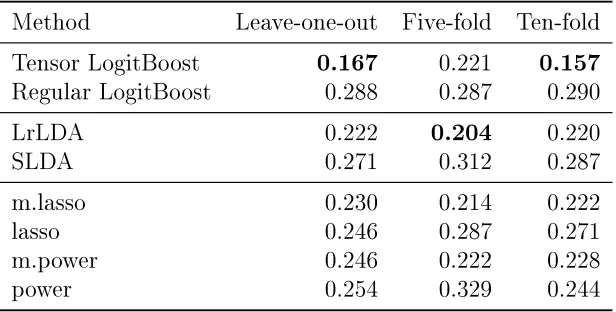
We reanalyzed the same EEG data set in Chapter 2 using the low-rank LDA and com-pared to the regular LogitBoost with the vectorized predictors, which is denoted as regular LogitBoost.

Instead of directly applying the classication method to the original EEG data, we preprocessed the data by tensor PCA to reduce the dimension. As for the evaluation of

the classication performance in Chapter 2, we partition the data into k ∈ {5,10,122}

portions. Each portion is held out once as the testing data set and the remaining k−1

portions together form the training data set. For the training set, a further ve-fold cross-validation is applied to choose the tuning parameters, including the number of boosting

stepsL, the rank of tensor regressionRand the shrinkage parameterν. We experimented

several scales of downsizing and obtained the similar results.

(59)

Table 3.1: Testing error for EEG data

Method Leave-one-out Five-fold Ten-fold

Tensor LogitBoost 0.167 0.221 0.157

Regular LogitBoost 0.288 0.287 0.290

LrLDA 0.222 0.204 0.220

SLDA 0.271 0.312 0.287

m.lasso 0.230 0.214 0.222

lasso 0.246 0.287 0.271

m.power 0.246 0.222 0.228

power 0.254 0.329 0.244

3.4 sMRI Data Analysis

3.4.1 Data Description

Attention decit hyperactivity disorder (ADHD) is one of the most commonly diag-nosed behavioral disorders among children. The primary symptoms for ADHD could be classied into three groups: developmentally inappropriate inattention, impulsive behav-ior and hyperactivity. Children with these symptoms do not know how to control their

behaviors or have trouble organizing their thoughts. About 5% of U.S. children aged

6-17 have been aected with ADHD (http://www.ncbi.nlm.nih.gov/pubmedhealth/ PMH0002518/). The levels of these primary symptoms are widely used as the diagnosis and treatment evaluation of ADHD. Ranking of these primary symptoms is often evalu-ated by the teachers or parents of the children, which is inherently subjective. Therefore, more objective methods are greatly desired.

(60)

(http://fcon_1000.projects.nitrc.org/indi/adhd200/). The ADHD-200 initiative organized the public release of the sMRI data and fMRI data for 776 children (285 children with ADHD and 491 controls) across 8 independent sites. A testing set of 195 unlabeled children then will be utilized to measure the performance of the classiers developed by the teams. Competition results have revealed that the prediction accuracy varied from

43.08%to61.54%with mean= 56.02%. The mean accuracy of predicting control subjects

is 71.77%, which is larger than the one of predicting children with ADHD (37.44%).

We only included the sMRI data in our analysis. The sMRI data set that we used is the preprocessed version of the ADHD-200 Global Competition sMRI data set, which is released by the Neuro Bureau (http://neurobureau.projects.nitrc.org/ADHD200/ Data.html). SPM8 is used for the preprocessing of the sMRI data (http://www.fil. ion.ucl.ac.uk/spm/software/spm8/).

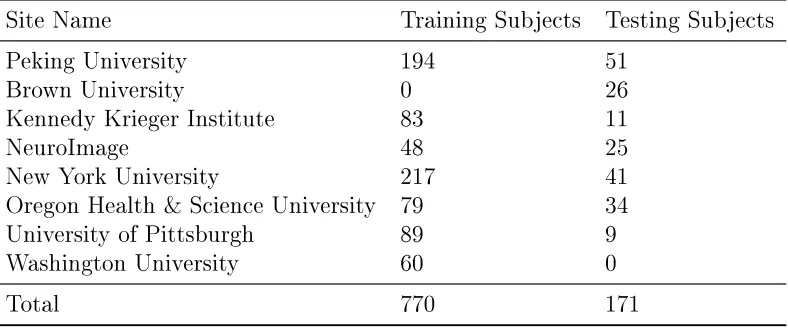
The preprocessed sMRI data comprises of 776 labeled children and 195 unlabelled children. The labeled training set contains 285 children with ADHD and 491 typical developed children (TDC). Not all the children in the training set and testing set were used for our analysis. For some children, the sMRI data are fragmentary and of low quality. Moreover, the diagnostic labels for the 26 participants from the Brown University are unavailable. It turns out that 770 training children and 171 testing children were used in our study. The number of children from each site is listed in Table 3.2.

3.4.2 Classication

Prior to classication, we performed the tensor PCA to downsize the sMRI data. The

original size of the sMRI data is121×145×121. We experimented four dierent scales of

(61)

Table 3.2: Training and testing subjects from dierent sites

Site Name Training Subjects Testing Subjects

Peking University 194 51

Brown University 0 26

Kennedy Krieger Institute 83 11

NeuroImage 48 25

New York University 217 41

Oregon Health &Science University 79 34

University of Pittsburgh 89 9

Washington University 60 0

Total 770 171

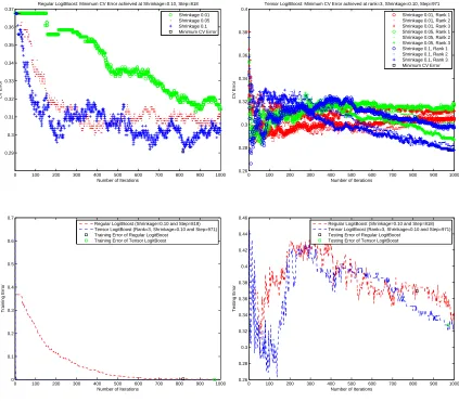
status based on the subject's downsized sMRI data. Figure 3.1, Figure 3.2, Figure 3.3 and Figure 3.4 present the analysis procedures for these four dierent versions of downsized sMRI data, which are described as follows. For the 770 training data, we employed a

ve-fold cross-validation to tune the number of boosting stepsL, the rank of tensor regression

R, and the shrinkage parameter ν in the tensor LogitBoost (upper-left panel). Also, L

andR in the regular LogitBoost were tuned using the same strategy (upper-right panel).

We then applied the tuned model to the testing data and evaluated the misclassication error rate (lower-right panel).

The classication errors on the testing set are reported in Table 3.3. Again, we observe superior performance of tensor LogitBoost compared to the regular LogitBoost. The

best prediction accuracy of 69.00% can be achieved when the 43×51×43 downsized

sMRI is used as the input of the tensor LogitBoost. Recall that the ADHD-200 global

competition results show that the prediction accuracy varied from 43.08% to 61.54%

(62)

0 100 200 300 400 500 600 700 800 900 1000 0.29 0.3 0.31 0.32 0.33 0.34 0.35 0.36 0.37

Number of Iterations

CV Error

Regular LogitBoost: Minimum CV Error achieved at Shrinkage=0.10, Step=818 Shrinkage 0.01 Shrinkage 0.05 Shrinkage 0.1 Minimum CV Error

0 100 200 300 400 500 600 700 800 900 1000 0.26 0.28 0.3 0.32 0.34 0.36 0.38 0.4

CV Error

Tensor LogitBoost: Minimum CV Error achieved at rank=3, Shrinkage=0.10, Step=971 Shrinkage 0.01, Rank 1 Shrinkage 0.01, Rank 2 Shrinkage 0.01, Rank 3 Shrinkage 0.05, Rank 1 Shrinkage 0.05, Rank 2 Shrinkage 0.05, Rank 3 Shrinkage 0.1, Rank 1 Shrinkage 0.1, Rank 2 Shrinkage 0.1, Rank 3 Minimum CV Error

0 100 200 300 400 500 600 700 800 900 1000 0 0.1 0.2 0.3 0.4 0.5 0.6 0.7

Training Error

Regular LogitBoost (Shrinkage=0.10 and Step=818) Tensor LogitBoost (Rank=3, Shrinkage=0.10 and Step=971)

Training Error of Regular LogitBoost Training Error of Tensor LogitBoost

0 100 200 300 400 500 600 700 800 900 1000 0.26 0.28 0.3 0.32 0.34 0.36 0.38 0.4 0.42 0.44 0.46

Testing Error

Regular LogitBoost(Shrinkage=0.10 and Step=818) Tensor LogitBoost(Rank=3, Shrinkage=0.10 and Step=971)

Testing Error of Regular LogitBoost Testing Error of Tensor LogitBoost