University of South Carolina
Scholar Commons
Theses and Dissertations
1-1-2013
Application of Agent-Based Approaches to
Enhance Container Terminal Operations
Omor Sharif Abul Bashar Mohammad
University of South Carolina - Columbia
Follow this and additional works at:https://scholarcommons.sc.edu/etd Part of theCivil and Environmental Engineering Commons
This Open Access Dissertation is brought to you by Scholar Commons. It has been accepted for inclusion in Theses and Dissertations by an authorized administrator of Scholar Commons. For more information, please [email protected].
Recommended Citation
APPLICATION OF AGENT-BASED APPROACHES TO ENHANCE CONTAINER TERMINAL OPERATIONS
by
Omor Sharif
Bachelor of Science
Bangladesh University of Engineering and Technology, 2006 Master of Science
University of South Carolina, 2011
Submitted in Partial Fulfillment of the Requirements for the Degree of Doctor of Philosphy in
Civil Engineering
College of Engineering and Computing University of South Carolina
2013
Accepted by:
Nathan Huynh, Major Professor Jonathan Goodall, Committee Member
Juan Caicedo, Committee Member Jose Vidal, Committee Member
c
Copyright by Omor Sharif, 2013
D
edication
A
cknowledgments
I would like to express my sincerest thanks to my committee chair Dr. Nathan Huynh who supervised, guided and supported me during the entire period. Without his help this dissertation would not be possible. I was fortunate to have accomplished faculties as committee members- Dr. Jon Goodall, Dr. Jose Vidal, Dr. Juan Caicedo and Dr. Chunyang Liu and I am indebted to them for much needed advice and feedback on my work. My special thanks to Dr. Vidal who has been enormously supportive and my source of expert opinions.
A
bstract
The globalization of trade and subsequent growth of containerization for trans-porting goods have brought many challenges for container terminals. Increasing demand, capacity constraints, lack of adequate decision making tools, congestion and environmental concerns are some of the major issues faced by container terminals today. Such terminals involve various processes in their operations and effective decision making is imperative in each process to manage scarce resources and improve the terminals’ competitiveness. This dissertation consists of research addressing three critical operational decision problems in marine terminal opera-tions involving application of agent-based modeling. The studies address 1) the truck queuing problem at terminal gates, 2) the inter-block yard crane scheduling problem and 3) the storage allocation problem. These problems share common objectives such as minimizing turn time of drayage trucks, reducing congestion and emission, and enhancing productivity of the terminals.
on the real-time feedback of congestion. Results from our experiments suggest that the proposed multi-agent framework can produce steadier truck arrivals at terminal gates and therefore significantly less average waiting time.
To facilitate vessel operations, an efficient work schedule for yard cranes is necessary given varying work volumes among yard blocks with different planning periods. The second study investigates an agent-based approach to assign and relocate yard cranes among yard blocks based on the forecasted work volumes. The objective of this study is to reduce the work volume that remains incomplete at the end of a planning period. Several preference functions are offered for yard cranes and blocks which are modeled as agents. These preference functions are designed to find effective schedules for yard cranes. In addition, various rules for the initial assignment of yard cranes to blocks are examined. The analysis demonstrated that the model can effectively and efficiently reduce the percentage of incomplete work volume for any real-world sized problem.
T
able
of
C
ontents
Dedication . . . iii
Acknowledgments . . . iv
Abstract . . . v
List ofTables . . . x
List ofFigures . . . xi
Chapter1 Introduction . . . 1
1.1 Research Topic I - Truck Queuing at Terminal Gates . . . 2
1.2 Research Topic II - Inter-block Scheduling of Yard Cranes . . . 2
1.3 Research Topic III - Storage Space Allocation in Yard . . . 3
1.4 List of Papers and Structure of Dissertation . . . 4
Chapter2 Background and LiteratureReview . . . 6
2.1 Flow of Containers in a Marine Terminal . . . 7
2.2 Processes in Container Terminals . . . 11
2.3 Research Trends in Container Terminals . . . 27
2.4 Contribution to Literature . . . 27
Chapter3 Application ofElFarolModel forManaging MarineTerminalGateCongestion . . . 30
3.1 Introduction . . . 31
3.3 Prior Research . . . 36
3.4 Methodology . . . 38
3.5 Experimental Design . . . 44
3.6 Results . . . 45
3.7 Conclusions and Future Work . . . 54
Chapter4 AnAgent-BasedSolutionFramework for Inter-Block YardCraneScheduling Problems . . . 57
4.1 Introduction . . . 58
4.2 Related Studies . . . 62
4.3 Methodology . . . 65
4.4 Implementation and Results from Experiments . . . 81
4.5 Conclusion and Future Work . . . 85
Chapter5 Storage SpaceAllocation at Marine ContainerTerminalsUsingAnt-BasedControl . . . 87
5.1 Introduction . . . 88
5.2 Review of Related Studies . . . 92
5.3 Methodology . . . 94
5.4 Model Implementation . . . 103
5.5 Experimental Design And Results . . . 105
5.6 Conclusion . . . 110
Chapter6 Conclusion . . . 111
L
ist
of
T
ables
Table 3.1 Values of parameters used in experiments. . . 45 Table 3.2 Mean wait, maximum wait and completiontime for tolerance,
L =10 minutes. . . 46 Table 3.3 Mean wait, maximum wait and completiontime for tolerance,
L =15 minutes. . . 47 Table 3.4 Mean wait, maximum wait and completiontime for tolerance,
L =20 minutes. . . 47 Table 3.5 Mean wait, maximum wait and completiontime for tolerance,
L =25 minutes. . . 47 Table 3.6 Mean wait, maximum wait and completiontime for tolerance,
L =30 minutes. . . 48 Table 3.7 Mean wait, maximum wait and completiontime for tolerance,
L =15 minutes (Asynchronous Case). . . 48 Table 3.8 Percentage decrease in emission. . . 54
Table 4.1 Values of parameters used in experiments. . . 83 Table 4.2 Percentage incomplete work volumes: Case I- Average number
of cranes per block = 1.0 . . . 84 Table 4.3 Percentage incomplete work volumes: Case II- Average
num-ber of cranes per block = 1.5 . . . 84
L
ist
of
F
igures
Figure 2.1 Container terminal subsystems (Modified from Henesey (2006)) 7 Figure 2.2 Flow of outbound/export containers (Modified from Rashidi
and Tsang (2006)) . . . 9
Figure 2.3 Flow of inbound/import containers (Modified from Rashidi and Tsang (2006)) . . . 10
Figure 2.4 A simplified three dimensional view of container terminal . . . . 10
Figure 2.5 Quay cranes working on a container vessel . . . 15
Figure 2.6 A straddle carrier . . . 17
Figure 2.7 An automated guided vehicle . . . 18
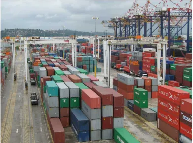
Figure 2.8 Container storage area . . . 20
Figure 2.9 Rubber tired yard cranes . . . 23
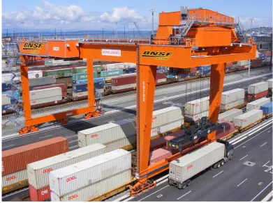
Figure 2.10 Rail-mounted yard crane . . . 23
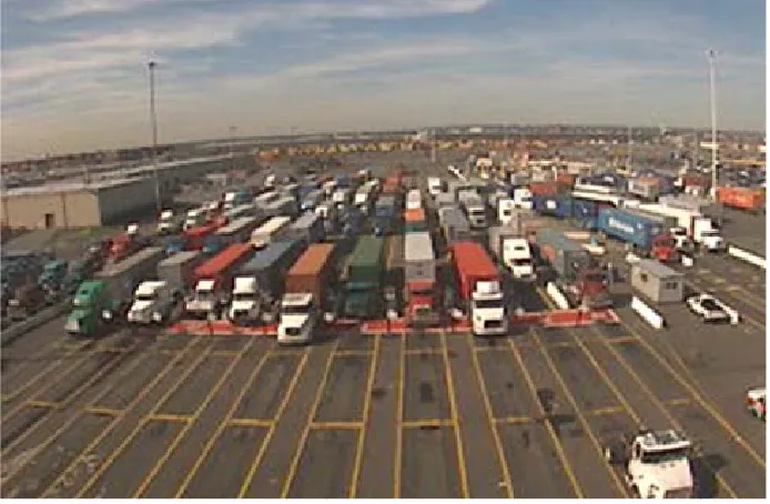
Figure 2.11 Trucks waiting at a container terminal gate . . . 26
Figure 3.1 Real-time view of gate condition via terminal webcam. . . 34
Figure 3.2 A screenshot of the Netlogo model evaluating terminal gate congestion. . . 43
Figure 3.3 Setting up the simulation. . . 43
Figure 3.4 Main loop of the simulation. . . 44
Figure 3.5 Impact of tolerance on mean wait time of trucks. . . 49
Figure 3.6 Impact of tolerance on maximum wait time of trucks. . . 50
Figure 3.7 Impact of tolerance on total completion time. . . 50
with 10 minutes tolerance. . . 52
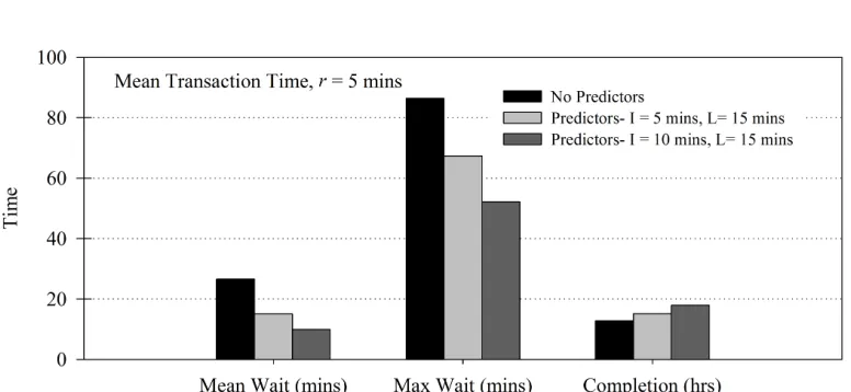
Figure 3.10 Results showing wait time and completion time with and without using predictive strategies. . . 53
Figure 3.11 Histogram of waiting time of truck forr = 5 minutes, I = 5 minutes, and L = 10 minutes. . . 53
Figure 4.1 Illustration of a container yard layout. (Not to scale) . . . 59
Figure 4.2 A rubber-tired yard crane on work. . . 60
Figure 4.3 Illustrating the transfer time of cranes. . . 67
Figure 4.4 A sample crane deployment scenario. . . 80
Figure 4.5 A screenshot of the agent-based model. . . 82
Figure 5.1 A schematic diagram of container terminal . . . 89
Figure 5.2 An illustration of ants in a network . . . 96
Figure 5.3 Relationship between update probability and age of ants . . . 99
Figure 5.4 Relationship between delay time and spare capacity of a block . 100 Figure 5.5 Influence between container routes, workload at blocks, pheromone tables and route of ants. . . 101
Figure 5.6 A screenshot of the agent-based model. . . 104
Figure 5.7 Convergence of container transport cost over time . . . 107
C
hapter
1
I
ntroduction
The globalization of trade and subsequent growth of containerization for transport-ing goods in containers have brought many difficulties and challenges in marine terminal operations. Capacity constraints, lack of adequate decision making tools, congestion and environmental concerns are some of the major issues faced by the container terminals today. Increasing containerization has also resulted in increased complexity in planning for terminal managers to provide satisfactory customer service and maintain terminals competitiveness. Various operations research optimization techniques, automated equipment and information tech-nology have become indispensable for efficient management of marine terminal operations and to attain high productivity in container flow with limited resources.
1.1 Research TopicI - TruckQueuing at TerminalGates
Queuing at marine terminal gates has long been identified as a source of emissions and high drayage costs due to the large number of trucks idling. The first study in this dissertation addresses queuing of trucks at marine terminal gates and presents a novel agent-based framework where the drayage companies can minimize congestion by using the provided real-time gate queuing information. The problem has been tackled based on the approach of El Farol Bar problem from game theory. Our proposed model can be used as a means of managing demand for the marine terminals, assuming that drayage firms will adjust their plans based on the real-time feedback of congestion. Results from our experiments suggest that the proposed multi-agent framework can produce more steady truck arrivals at terminal gate and therefore significantly less average waiting time.
Readers are referred to Chapter 3 of this dissertation for more information about this work, which provides an overview of the truck queuing problem and illustrates how the El Farol Bar problem is adapted as a multi-agent solution framework. A review of related studies is included along with formulation and implementation of the proposed model. Experimental designs of test problems and results are presented to demonstrate the effectiveness of the proposed framework.
1.2 Research TopicII - Inter-blockScheduling of YardCranes
incomplete at the end of a planning period. Several preference functions are offered for yard cranes and blocks which are modeled as agents. These preference functions are designed to find effective schedules for yard cranes. In addition, various rules for the initial assignment of yard cranes to blocks are examined. The analysis demonstrates that the model can effectively and efficiently reduce the percentage of incomplete work volume for any real-world sized problem.
Readers are referred to Chapter 4 of this dissertation for more information about this work, which describes the interblock yard crane scheduling problem and illustrates our proposed methodology in detail regarding the assumptions and the steps of analysis. It also provides a review of related studies and a sample example to demonstrate the approach. The test results from the model based on various real-world sized crane deployment problems are included and results show that the model provides excellent solutions in short time for a range of work volume conditions with high variation.
1.3 Research TopicIII - Storage SpaceAllocation inYard
The results from experiments show that the proposed approach is effective in balancing the workload among yard blocks and reducing the distance traveled by internal transport vehicles during vessel loading and unloading operations.
Readers are referred to Chapter 5 of this dissertation for more information about this work. It describes the storage space allocation problem and its importance. In addition to a review of related studies, all necessary detail of the ant-based control method is presented. Then the model implementation steps are illustrated with experimental designs. Finally, the relevant results and the contributions from this research are included. Simulation results show that the proposed approach effectively balances the workload among yard blocks and thus minimizes congestion on the road network for trucks and yard cranes. At the same time, the transport distance of containers between yard blocks and berth is minimized.
1.4 List ofPapers andStructure ofDissertation
This dissertation includes three research projects completed and published in peer-reviewed journals and these journal articles appear in the dissertation as separate chapters. They
are-1. Sharif, O., N. Huynh and J. M. Vidal (2011). Application of El Farol Model for Managing Marine Terminal Gate Congestion. Research in Transportation Economics, 32(1), 81-89.
2. Sharif, O., N. Huynh, M. Chowdhury, and J.M. Vidal (2012). An Agent-Based Solution Framework for Inter-Block Yard Crane Scheduling Problems. International Journal of Transportation Science and Technology, 1(2), 109-130.
C
hapter
2
B
ackground and
L
iterature
R
eview
This chapter aims to provide a broad overview of marine terminal and its opera-tions. The chapter also presents a selection of related studies. A comprehensive review of literature on the two completed studies that are included in this disserta-tion can be found in the respective journal article chapters.
SHIP TO/FROM
BERTH
TRANSFER OPERATIONS
STORAGE
OPERATIONS DELIVERY/RECEIPT
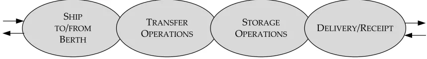
Figure 2.1 Container terminal subsystems (Modified from Henesey (2006))
container ships and container terminals are often expressed in TEUs. According to Zhang et al. (2002), the main functions of container terminals are delivering con-tainers to consignees and receiving concon-tainers from shippers, loading concon-tainers onto and unloading containers from vessels and storing containers temporarily to account either for efficiency of the deployed equipment or for the difference in arrival times of the sea and land carriers.
Marine container terminals operate under several performance goals but the primary objective is to achieve rapid flow of containers at a minimum cost. In this context, the time to load/unload a ship (the time spent by a ship at berth, also known as ‘turn time’) has been generally regarded as a measure of container terminal efficiency. Therefore, much research has been focused on the ‘marine side’ interface of a container terminal, which leaves room for further research such as the ‘land side’ interface (Henesey, 2006).
2.1 Flow ofContainers in a MarineTerminal
The flow of containers in a marine terminal can be viewed as being composed of four broad subsystems. Each container, whether an import container or an exportcontainer, goes through these subsystems between the ship and designated customer/consignee located on land. These subsystems are shown in Figure 2.1.
and Receipt’ indicates that a container is delivered to the port by a customer for export or an import container is picked up by a consignee from the port. The two directional arrows in Figure 2.1 indicate that the direction of flow of import and export containers is reverse to one another. Each of these subsystems has a container handling capacity based on their operational strategy and resources deployed. The subsystems all together determine the performance of the container terminal. A bottleneck in any of these subsystems will increase containers transfer time and consequently impact the productivity of terminal and customer service. Also, the interaction and coordination among the four components are critical for the overall performance. However, to date most of container terminal research has focused on the subsystems individually with very few on the whole system or from a ‘holistic’ view (Henesey, 2006).
Customer/ Depots
Terminal Gate
Storage Area/
Container Yard Shore/Berth Vessel/Ship
XTs: External Trucks YCs: Yard Cranes
AGVs: Automated Guided Vehicles ITs: Internal Trucks
SCs: Straddle Carriers
XTs AGVs/ ITs/ SCs
XTs YCs QCs
Container Arrival And Storage Container Retrieval And Loading
Customer/ Depots
Terminal Gate
Storage Area/
Container Yard Shore/Berth Vessel/Ship
XTs AGVs/ ITs/ SCs
XTs YCs QCs
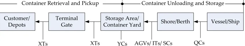
Container Retrieval and Pickup Container Unloading and Storage Figure 2.2 Flow of outbound/export containers (Modified from Rashidi and Tsang (2006))
Rushton et al. (2010) and Henesey (2006) present some typical issues addressed in each level of decisions. Strategic level typically involves choice of a terminal location, terminal size, resource types etc. Tactical level typically involves alloca-tion of resources, determining size of workforce etc. Operaalloca-tional level typically involves daily scheduling of jobs, equipments, process management, scheduling of workers, etc.
Since marine terminals serve as an intermodal service for transferring contain-ers between ocean and land, their primary purposes are 1) to receive outbound containers from customers for loading into vessels and 2) to unload inbound containers from vessels for picking up by consignees (Rashidi and Tsang, 2006). These operations are known as export and import processes respectively and the containers are identified as import container (or inbound container) and export container (outbound container). The flows of outbound and inbound containers are illustrated in Figure 2.2 and Figure 2.3. Also, a three dimensional representation of container terminal is shown in Figure 2.4.
con-Customer/ Depots
Terminal Gate
Storage Area/
Container Yard Shore/Berth Vessel/Ship
XTs: External Trucks YCs: Yard Cranes
AGVs: Automated Guided Vehicles ITs: Internal Trucks
SCs: Straddle Carriers
XTs AGVs/ ITs/ SCs
XTs YCs QCs
Container Arrival And Storage Container Retrieval And Loading
Customer/ Depots
Terminal Gate
Storage Area/
Container Yard Shore/Berth Vessel/Ship
XTs AGVs/ ITs/ SCs
XTs YCs QCs
Container Retrieval and Pickup Container Unloading and Storage
Figure 2.3 Flow of inbound/import containers (Modified from Rashidi and Tsang (2006))
476 T.G. Crainic and K.H. Kim
Fig. 2. Example of a container terminal with an indirect transfer system (Park, 2003).
tainers between the three areas. Figure 2illustrates part of a container port terminal. One ship and three quay cranes are displayed in the sea-side area, while only trucking is shown in the land-side area. Twelve container stacks are displayed in the yard area, as well as one type of yard crane used to transfer containers between yard transporters and outside trucks and stacks, as well as to change the position of containers in the yard as required.
Three main types of handling operations are performed in a container ter-minal:
(1) ship operations associated with berthing, loading, and unloading con-tainer ships,
(2) receiving/delivery operations for outside trucks and trains, and (3) container handling and storage operations in the yard.
When a ship arrives at the container port terminal, it is assigned a berth and a number of quay cranes. Berth space is a very important resource in a container terminal (construction costs to increase capacity are very high, even when space for growth exists) andberth schedulingdetermines the berthing time and position of a container ship at a given quay (Section 5.1). Quay-crane alloca-tionis the process of determining the vessel that each quay crane will serve and the associate service time (Section5.2).Stowage sequencingdetermines the
se-Figure 2.4 A simplified three dimensional view of container terminal
tainers. However since the operational strategy varies among container terminals the choice of equipments deployed may also vary accordingly. The role of these of equipments in various processes within a container terminal will be briefly illustrated in Section 2.2.
2.2 Processes inContainerTerminals
et al. (2007) used five types of decision problems which are berth allocation, quay crane scheduling, yard operations, transfer operation and ship stowage planning. The different classification proposed by different authors originate from how they prefer to view or classify port operations. This dissertation assumed six subclasses of decision problems in container terminal and each of them are reviewed briefly in following sections.
Berth allocation
Following the arrival of a ship at port, it must be allocated a place at the quay where it can moor. The places where ships can moor are known as berths. The problem of berth allocation involves assigning a berth to an arriving ship such that the allocation maximizes utilization of berths. Some of the issues that are considered in berth allocation include length of ship, depth of berth, ship’s timing window, priorities and berthing preferences, location of berth with respect to stacking area where containers for a particular ship are stored etc. While berth allocation is a decision made at operational level, how many berths should be available at the quay is a part of decision making at strategic level. Berths are critical resources in that they directly relates to capacity of the terminal. Also, the construction of berths entails very high cost relative to the investment made in the other facilities in the port (Park and Kim, 2003).
Quay crane scheduling
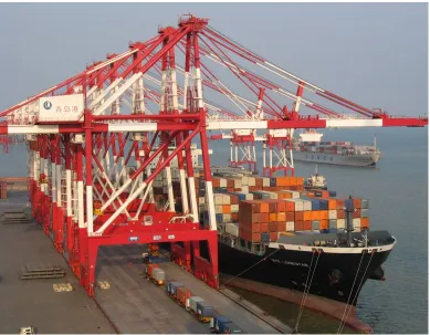
After a ship is docked at a berth, unloading and loading of containers will begin. For this purpose, a number of Quay Cranes (QCs) is assigned to a ship. QCs unload the import containers from ship’s deck to shore. The QCs will place the containers to transfer vehicles which travel between the QCs and container stacking area. For export containers, QCs will load them on the ship from the transfer vehicles. Figure 2.5 shows typical QCs deployed at container terminal. Quay Crane scheduling problems involve determining how many QCs will be assigned to a ship and the set of jobs (loading and unloading moves) that will be performed by a QC. Most often the objective of QC scheduling problem is to minimize the time required to unload and load a ship, thereby minimizing ship’s turnaround time. The constraints considered are interference between the QCs, precedence relationships among the containers etc. In general, sequence of unloading operations of containers offers more flexibility compared to loading operations since a good distribution of containers over the ship is necessary. A desired distribution of containers is accomplished by ‘stowage planning’ which is the problem of allocating space to outbound containers on the board of a ship. Stowage planning is influenced by size/type/weight of containers, the ports the ship will be visiting etc. It should be noted that berth allocation and QC scheduling are sometimes considered simultaneously since the berthing time of a ship is in turn dependent of efficient schedules of QCs.
Figure 2.5 Quay cranes working on a container vessel
is introduced to solve for optimal solution. To overcome computational difficulty of the branch and bound method a heuristic search algorithm was also developed. Moccia et al. (2006) developed a branch-and-cut algorithm for large sized schedul-ing problems as to minimize the vessel completion time as well as the crane idle times. Sammarra et al. (2007) decomposed the quay scheduling problem into two parts- routing problem and scheduling problem. The routing problem is solved by tabu search heuristic and a local search technique is used to generate the solution of the scheduling problem.
Transport of containers to stack and vice versa
Figure 2.6 A straddle carrier
shows a typical AGV. Once what type of equipment will be used for transport is made at strategic level, how many of these equipments is necessary is decided at the tactical level. At the operational level, scheduling and routing of containers are addressed ı.e. which container will be handled by which equipment and which path is chosen. Transport operations are usually optimized to minimize number of vehicles, idling of cranes and vehicles, distance traveled by vehicles etc. Some researchers tackled scheduling problem along with storage space allocation of a container (location of a container in yard) as an integrated process. Storage space allocation problem is reviewed in the next section.
con-Figure 2.7 An automated guided vehicle
and terminal layout on terminal performance. Two terminals with different but commonly used yard configurations are considered for automation using AGVS. A multi attribute decision making method is used to investigate the performance of the two terminals and determine the optimal number of deployed AGVs. Vis et al. (2005) proposed to introduce buffer areas at both quay side and yard side for decoupling of the unloading and transportation processes. The objective is to minimize the vehicle fleet size such that the buffer areas do not exceed their capacity. An integer linear program was developed and simulation was used to verify the analytical results. Cheng et al. (2005) proposed a network flow model taking into account the impact of congestion. The objective is to find a suitable number of AGVs to be deployed and minimize their idling time at berth.
Yard operations - Storage space assignment
Figure 2.8 Container storage area
consists of several rectangular storage blocks known as yard blocks. A typical yard block is 40 forty-footbays/slotslong. Each bay is 6rowswide, and containers can be stacked up to 4tiers. Tiers refer to the height to which containers are stacked. The objective of storage space assignment is to determine an optimum space allocation such that handling and rehandling of containers is kept at minimum and traveling time of vehicles is minimized. Thus some researchers have tackled the storage assignment problem along with transportation planning problem.
in connection with unproductive moves of outbound containers. A binary linear program and a heuristic approach are developed. Zhang et al. (2003) decomposed the storage space allocation problem into two levels and each level is formulated as a mathematical programming model. At the first level, the total number of containers to be placed in each storage block is set to balance workloads among blocks. The second level determines the number of containers associated with each vessel that constitutes the total number of containers in each block in each period. The objective is to minimize the total distance to transport the containers between their storage blocks and the vessel berthing locations. Kang et al. (2006) proposed a method based on a simulated annealing search to derive a good stacking strategy for containers with uncertain weight information. Simulation experiments are used to show that the strategies effectively reduce the number of rehandlings. Lee et al. (2007) studied the storage allocation problem to efficiently transport containers between the vessels and the storage area so that reshuffling and traffic congestion is minimized. To reduce reshuffling, unloaded containers are grouped according to their destination vessel. To reduce traffic congestion, a workload balancing protocol is proposed. Two heuristics are also developed- the first is a sequential method while the second is a column generation method. Lee and Hsu (2007) proposed an optimization model for the container pre-marshalling problem. To minimize the reshuffling, the authors attempted to pre-marshall the containers in such a way that it fits the loading sequence of containers on a vessel.
Yard operations - Yard crane scheduling
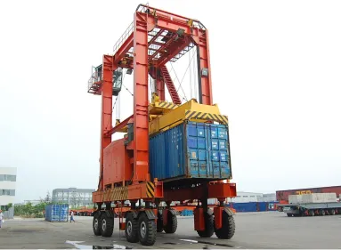
Tsang, 2006). In previous section, we reviewed container storage space assignment problem and this section will briefly discuss the scheduling of equipments that are deployed for container storage and retrieval operations. The equipments are used for loading, unloading, rehandling/reshuffling of containers. Choice of equipments for handling of containers is a decision that is made at strategic level. For this purpose forklift trucks, reach stackers, yard cranes are available options. Commonly used yard cranes are Rail Mounted Gantry Cranes (RMGCs) and Rubber Tired Gantry Cranes (RTGCs). Straddle Carriers (SCs) are also a feasible choice and they are reviewed in Section 2.2. RMGCs are also known as Automated Stacking Cranes (ASCs) and they move on rails and can provide high density storage. However, RMGCs can only travel in one direction across the stacks. An RMGC is shown in Figure 2.10. RTGCs, in contrast, are rubber tired and offer more flexibility. RTGCs are popular and more frequently used in large terminals with high container flows and other automated technologies (Henesey, 2006). A typical RTGC is shown in Figure 2.9. The objective of crane scheduling is to maximize utilization of cranes and minimize the waiting time of transport vehicles (ITs, XTs, AGVs etc). The workload at different blocks within a yard changes over time and scheduling must ensure that more cranes are deployed at blocks with heavier workloads. The typical constraints in a scheduling problem are traffic congestion and interference among cranes.
Figure 2.9 Rubber tired yard cranes
handled.
Delivery and receipt operations
Export containers are brought into the port and import containers are picked up from the port by external trucks (XTs). For both delivery and receipt operations, external trucks (also known as drayage trucks) have to pass through terminal gates for documentation processing, inspection, security checks etc. The objective of optimizing delivery and receipt operations is to minimize the turn time of drayage trucks. The turn time of drayage trucks primarily consists of two components-waiting at gate and components-waiting at yard. Figure 2.11 shows trucks wating at a terminal gate. Idling at yard implies waiting for a yard equipment to come to the truck and load/unload the container to/from the truck. Also, long queue of trucks at terminal gates is a concern since it leads to larger turn time and emission due to congestion. In recent years, some ports have adopted appointment/reservations systems to reduce queuing at gates, where truckers select from a given list of available time windows to arrive to pickup or deliver their containers. However, studies indicate that current appointment strategies have not improved the queu-ing situation. Because of the lack of specific guidelines for implementqueu-ing the appointment systems and that each terminal is left to manage their own system, the lack of structures in the appointment system has led to little time savings for truckers as reported in the work of Giuliano and O’Brien (2007). Another approach being experimented by some terminals is to provide live views of their gates via webcams. However, no guidelines or studies are available how to utilize this information to the benefit of truck dispatchers.
Figure 2.11 Trucks waiting at a container terminal gate
Huynh and Walton (2008) determined the maximum number of trucks a terminal operator could allow into its terminal based on available resources and investigated the effect of limiting the truck arrivals on the terminal’s throughput and resource utilization. In a related study, Huynh (2009) explored rules for scheduling trucks to minimize total delays to trucks. Guan and Liu (2009) utilized a multi-server queuing model to analyze marine terminal gate congestion and quantified truck waiting cost. In the same study, they proposed an optimization model to balance the gate operating cost and truckers’ cost due to excessive waiting time.
windows for cargo delivery/pickup at marine container terminals taking into account the objectives and constraints of the terminal operator and freight carriers.
2.3 Research Trends inContainer Terminals
There is a large amount of literature in the area of marine container terminal modeling. As the container terminal operations are becoming more and more important, the numbers of publications appearing in literature are also increasing. In most instances, operation research optimization methods such as mathematical programs and meta-heuristics are employed by researchers to tackle the container terminal decision problems. Research papers on container terminals can be dis-tinguished in three classes: a) an intensive study or sophisticated model of a single process or decision problem, b) two or more related decision problems as an integrated process or model c) model of an entire container terminal as a coordinated system of container flow. To date, the approach of independent decision problems is most common where a particular operation is optimized rather than integrating several processes or optimizing the whole system. However, more efficiency can be achieved when related processes in terminal operations are considered together. The few studies available in literature adopting integrative views applied analytical, simulation and multi-agent approaches.
2.4 Contribution toLiterature
and enhancing the productivity of terminals. The research carried out in this dissertation contribute to the container terminal literature on both land and water side interface operations. Much research has been focused on the marine side interface of a container terminal, however, the land side interface has not received adequate attention until recently as the environmental issues and high drayage cost have become major concerns. Also, the contribution of the dissertation is important in that all of the papers involve investigation of applicability of agent-based approaches. Agent-agent-based modeling is a new paradigm being introduced to container terminal operations. More specific contribution to literature made by the three research papers are briefly discussed in the following sections.
Study on ‘Truck queuing at terminal gates’
The contributions of this study to literature are: 1) it is the first study to analyze the potential benefits or adverse effects of providing real-time gate congestion information, 2) it examines ways in which the dispatchers and truckers could take advantage of the provided real-time information such that their collective truck queuing time is minimal, and 3) it presents an agent-based framework to be used by truck dispatchers to achieve steady arrival of trucks and hence less queuing at terminal gates.
Study on ‘Inter-block yard crane deployment’
Study on ‘Storage space allocation problem’
C
hapter
3
A
pplication of
E
l
F
arol
M
odel for
M
anaging
M
arine
T
erminal
G
ate
C
ongestion
1Abstract
Truck queuing at marine terminal gates has long been recognized as a source of emissions problem due to the large number of trucks idling. For this reason, there is a great deal of interest among the different stakeholders to lessen the severity of the problem. An approach being experimented by some terminals to reduce truck queuing at the terminal is to provide live views of their gates via webcams. An assumption made by the terminals in this method is that truck dispatchers and drivers will make rational decisions regarding their departure times such that there will be less fluctuations in truck arrivals at the terminal based on the live information. However, it is clear that if dispatchers send trucks to the terminal whenever the truck queues are short and not send trucks when the truck queues are long, it could lead to a perpetual whip lash effect. This study explores the predictive strategies that need to be made by the various dispatchers to achieve the desired effects (i.e. steady arrival of trucks and hence less queuing at the seaport terminal gates). This problem is studied with the use of an agent-based simulation model and the solution to the well known El Farol Bar problem. Results
1O. Sharif, N. Huynh, J. M. Vidal,Research in Transportation Economics, 2011, Volume 32, Issue 1,
demonstrate that truck depots can manage (without any collaboration with one another) to minimize congestion at seaport terminal gates by using the provided real-time gate congestion information and some simple logics for estimating the expected truck wait time.
Keywords: Drayage operations, truck queuing, terminal webcams, multi-agent systems, simulation, and El Farol Bar problem.
3.1 Introduction
Port drayage is defined as a truck pickup from or delivery to a seaport, with the trip origin and destination in the same urban area is a critical, yet comparatively understudied link in the intermodal supply chain (Harrison et al., 2007). Despite the relatively short distance of the truck movement compared to the rail or barge haul, drayage accounts for a large percentage, between 25% and 40%, of origin to destination expenses (Macharis and Bontekoning, 2004). High drayage costs seriously affect the profitability of an intermodal service which in turn could impede the advance of intermodal freight transportation. Hence, it is important to improve drayage operations to keep costs low. Another important reason to improve drayage operations is to reduce its emissions impact on the surrounding communities due to engine idling and the stop-and-go lugging. Reducing the idling time of drayage trucks is equivalent to reducing local and regional particulate matter (PM 2.5), nitrogen oxides, and greenhouse gas emissions. Because drayage trucks operate primarily in urban environments, a reduction of these harmful pollutants has a proportionally greater benefit.
drayage trucks is simply a function of supply (terminal resources) and demand (number of trucks). Given that resources (e.g. gates, clerks, yard cranes) at a terminal change very little on any given day, excessively long turn time for trucks is often the result of fluctuating truck arrivals. That is, because trucks come to the terminal at their earliest convenience without any prior announcement of their arrivals to the terminal operator, there are times during the day where the number of waiting trucks (demand) greatly exceeds the terminal’s resources (supply). When demand greatly exceeds supply, truckers are forced to wait for their turn, resulting in engine idling and stop-and-go lugging. It should be noted that the truck arrivals are driven by shipper demands and ship schedules. Thus, there is a rational explanation for the observed peaking of truck traffic at the terminals.
One solution to the fluctuating truck arrivals is to employ an appointment system whereby the terminal operator designates available time windows for containers and subsequently truckers choose one of the available time windows. With an appointment system, the terminal operator could effectively control the truck arrival rates to keep its resources operating at the maximum level while at the same time ensuring timely service to the trucks. Recognizing the potential of this system, legislation in California suggested terminals to adopt the appointment system, among other methods, in an effort to reduce the number of trucks idling (California Assembly Bill 2650); the stated goal of this regulation was to reduce emissions. A subsequent bill (AB 1971) was passed in the summer of 2004 to include truck queuing. Hence, terminals in Los Angeles, Long Beach, and Oakland are subject to a $250 fine for each truck idling or queuing for more than 30 minutes while waiting to enter the terminal gate. Appointment systems are also employed by terminals outside of California (e.g. Port of Vancouver) and are under consideration at other US terminals.
and reduce trucks’ turn time. However, in practice, because of the lack of specific guidelines for implementing the appointment systems and that each U.S. terminal is left to manage their own system, the lack of structures in the appointment system has led to little time savings for truckers as reported in the work of Giuliano and O’Brien (2007). A similar conclusion was reached in a recently completed federal study which stated that “appointment systems are in an early stage of development, with no uniformity between terminals or ports and many implementation issues to be resolved” (Tioga Group et al., 2011). This problem of inefficiencies due to poor scheduling produce congestion, port staff overloads, unmet trucker needs, and general frustration. Given the present situation of high fuel costs and rising trucker discontent with port congestion, terminal operators seek to utilize as many low-cost solutions as possible. One such low-cost solution is to provide a live view of the gate condition via a webcam that can be accessible via the Internet. Implicitly, the terminal operators are assuming that dispatchers and truckers will utilize the provided information to their advantage; that is, not come during the peak periods. Hence, it is assumed that the truck arrival rates will have less variance and thereby reduces truck queuing at the terminal gates. To our knowledge, no research has been conducted to analyze the potential benefits or adverse effects of providing real-time gate congestion information. Through the use of agent-based simulation, this study seeks to examine ways which the dispatchers and truckers could take advantage of the provided real-time information such that their collective truck queuing time is minimal.
3.2 Background andProblemDescription
Figure 3.1 Real-time view of gate condition via terminal webcam.
monitor the gate congestion condition and depending on the congestion level at the gate will send or withhold a truck at the depot. For example, if the dispatchers see that the terminal is busy, as shown in Figure 3.1, he/she may elect to have the truck make another move elsewhere instead of sending the truck to the terminal where it will likely have to wait for an extended period of time before receiving service. There are two important factors that affect the dispatcher’s decision making. The first is the method which he/she uses to predict the expected waiting time for the truck when it gets to the terminal, and the second is the tolerance level that determines whether or not to send the truck.
The decision making process by the truck dispatchers is similar to that of individuals in the El Farol Problem. A brief summary of the El Farol Bar Problem and its solution are presented here. For additional details, readers are referred to the seminal work of Arthur (1994).
evening would only be enjoyable if the bar is not too crowded, say 60 people or fewer. There is no way to tell the numbers coming in advance; therefore, a person or agent goes to the bar if he expects fewer than 60 to show up or stays home if he expects more than 60 to go. Choices are unaffected by previous visits. There is no collusion or prior communication among the agents, and the only information available is the numbers who attended in past weeks.
Assume agents can individually form several predictors in the form of functions that map the past d weeks’ attendance figures into next week’s. Suppose recent attendance to the bar is:
...44, 78, 56, 15, 23, 67, 84, 34, 45, 76, 40, 56, 22, 35.
Possible predictors are: the same as last week’s (35), a mirror image around 50 of last week’s (65), or an average of the last four weeks (49).
The person decides to go or stay according to the currently most accurate predictor in his set. Once decisions are made, he learns the new attendance figure and updates the accuracies of his monitored predictors. In this bar problem, the set of predictors currently most credible and acted upon by the agents determines the attendance. But the attendance history affects the agents’ set of predictors.
extended Arthur’s work to the gate congestion problem.
The terminal gate congestion problem addressed in this study seeks to under-stand the effects the predictive strategies, tolerance level, and operational related parameters have on the truck waiting time. Our goal is to design a decision making framework for the truck dispatchers that would produce steady demand at the marine terminal gate and also minimize waiting time for all trucks. It should be noted that the problem addressed in this study is more complex than the original El Farol Bar Problem. First, the total demand (number of people intending to go to the bar) does not vary with time, whereas the truck demands vary throughout the day. Second, the bar attendance event occurs at one specific time. In contrast, truck dispatching a continuous process that occurs throughout the operational hours of the terminal. Third, depots are not homogenous in that they are located at different distances to/from the terminal; depots that are closer to the terminal require less travel time to the terminal and hence are in a better position to take advantage of the provided real-time information because their expected wait time, E(W) will be closer to the actual wait time. Fourth, drayage operations involve travel time and service time; these parameters are not applicable in the bar problem. Given that service time is stochastic, the predictive strategy of estimating truck wait time based on information is more difficult. In summary, terminal gate congestion problem addressed in this study is more complex in nature than the original El Farol Bar problem and thus finding the near-optimal solution is more challenging.
3.3 PriorResearch
is limited work that deals specifically with strategies for managing marine terminal gate congestion. These works are addressed from either the drayage operator’s or terminal operator’s perspective. From the terminal operator’s perspective, managing gate congestion can be accomplished via the use of a truck appointment system where truckers select from a given list of available time windows to arrive to pickup or deliver their containers. The terminal operators can better manage their workloads by controlling and limiting the available time windows. Work in this area include a study by Huynh and Walton (2008) who determined the maximum number of trucks a terminal operator could allow into its terminal based on available resources and investigated the effect of limiting the truck arrivals on the terminal’s throughput and resource utilization. In a related study, Huynh (2009) explored rules for scheduling trucks to minimize total delays to trucks. Guan and Liu (2009) utilized a multi-server queuing model to analyze marine terminal gate congestion and quantified truck waiting cost. In the same study, they proposed an optimization model to balance the gate operating cost and truckers’ cost due to excessive waiting time.
Multi-Agent Systems (MAS) has become an important field within artificial intelligence research, and it has been successfully applied to applications such as control processes, mobile robots, air traffic management, and intelligent in-formation retrieval. Far fewer applications are found in the areas of freight and intermodal transportation, in particular, seaport container terminals. To our knowl-edge, no study has examined the marine gate congestion problem from the MAS perspective.
3.4 Methodology
This section provides details regarding our formulation and implementation.
Formulation
A formal description of the problem is given here. There is a set of depots N and each depotn ∈ N has a set of trucksT to send to the port in the planning period; the availability of containers (ready time for pick up of a container) associated with trucks follow a Poisson distribution with a mean of θ. All trucks are sent
dispatch truckt to the port or 0 if it decides to withhold the truck. Once truckt is dispatched, it undergoes three different processes before it enters the terminal. The first process is making the trip to the port which takes time T(t,P). Once a truck arrives in the vicinity of the gates, it picks a lane to enter. Here, we assume that truckers will select the lane with the shortest physical queue length (least number of trucks waiting in a lane). The second process is waiting in the queue. The actual queuing time of truck t is denoted as Q(t). Q(t) begins the instant when a truck joins the back of a queue and ends when the immediate preceding truck finishes its transaction. If no queue is present,Q(t) =0. The third process is receiving service such as documentation processing at the gate. The service time of truck tis denoted asS(t) which follows the Exponential distribution with mean r. A truck’s wait time, W(t), is(Q(t) +S(t)).
The dispatchers at depots make the SEND?(n,t) decision such that its truck can avoid excessive waiting at the terminal gate. The depot agents seek to accomplish this objective without any communication or collusion with other agents. In other words, the function SEND?(n,t) is internal to depot agents and its value is not disclosed to other agents when the decision is made. As previously defined, for all agents excessive wait time occurs when E(W)> L. The study period is discretized into uniform time intervals of length I. LetKbe the number of trucks that finished their transactions at the gate during interval x. We defined the average truck wait time,Wx during the xth interval as follows.
Wx = ∑ K
k=1W(k)
K (3.1)
Historyx ={Wx−m, ...,Wx−2,Wx−1} (3.2)
However, it is possible that no trucks finished its transaction during interval x. In this scenario, we use a real-time estimate of truck wait time using a snapshot of the current demand at the gate. For instance, if at the beginning of xth time intervalWx−1 is not available, then we computeWx−1 as follows.
b
Wx−1 = (Nq+1)×r (3.3)
where Nq is the number of trucks in the shortest queue at the current time. Using the historical truck waiting time, at some xth interval, the agents would estimate the time its truck has to wait at gate if it is dispatched at the onset of xth interval,E(W). Note that the agents do not know the trueWxuntil (x+1)th interval. Depot agents carry out this prediction with the aid of internal models calledpredictors. Predictors are simple rules or logic (inductive reasoning) that can provide an estimate of E(W) based on past trends or independently of past history. We use a large set of global predictor space, S= [s1,s2,s3, ...,sz], which contains z predictors in total. Each depot agentn ∈ N chooses randomly a fixed number of predictors, sayk, fromSand keeps a list of these predictors in my-predictors-list(n). However, as time progresses, agents learn how well each of his predictors is performing and will subsequently rank its predictors. The ranking information is recorded in a list named my-predictors-scores(n). This list maps score for each predictor into my-predictors-list(n). Also, all depot agents keep another list named my-predictors-estimates(n) that records estimates ofWx using each predictor in my-predictors-list(n). Note that the length of all three lists for each agent will be equal to k.
active predictor and is denoted as sactive−predictor(n). The predicted value of Wx using sactive−predictor(n) is denoted as E(W). In deciding whether to send the truck at the xth interval, the depot agent applies the following logic.
1 ifE(W) ≤L
2 thenSEND?(n,t) = 1 3 else SEND?(n,t) = 0
The global set of predictor models, S, employed in our work closely follows the set of strategies used by Garofalo (2006). A brief description of these strategies is given below:
• TitForTat: This family of strategies predicts next interval’s attendance by using the same value asuweeks ago, with ufrom 1 tom.
• Mirror: This is a family of strategies using a mirror image around 50% of 2L, with 1 to mintervals ago.
• Fixed: The Fixed strategy always chooses the same wait time estimate (10%, 20%, 30% ... or 200% of L).
• Trend: A u(1 tom) dated 2 intervals trend applied to the last interval.
• OppositeTrend: Au (1 tom) dated 2 intervals opposite trend applied to the last interval.
• Trend2: A u (1 tom) dated 2 intervals (3 interval spaced) trend applied to the last interval.
• MovingAverage: Au(1 to m) 5 intervals moving average.
• Trend3: A u (1 to m) dated 2 intervals relative trend applied to the last interval.
• OppositeTrend3: Au (1 tom) dated 2 intervals relative trend applied to the last interval.
To update the performance (score) of the predictors in my-predictors-scores(n) which is subsequently used to determine sactive−predictor(n), the three methods that are discussed in the literature are: absolute precision, relative precision, and original precision (Garofalo, 2006). In this study, we adopted the original precision approach. This approach was applied by Zambrano (2004), and according to him the evaluation function is the same as that was used in Arthur’s seminal work. The original precision score updating method has the following form.
Ux(xj(n)) = α∗Ux−1(sj(n)) + (1−α)|wnx(sj(n))−wx| (3.4)
where Ux(xj(n)) is the score of predictor j at xth interval owned by agent n. wnx(sj(n))is the truck wait time estimation by predictor jatxthinterval by agent n. wx is the actual wait time atxth interval. α is a number strictly between zero and
one. A lowα gives more importance to recent performance while a high α gives
more importance to past performance.
Implementation in Netlogo
Figure 3.2 A screenshot of the Netlogo model evaluating terminal gate congestion.
setup()
1 create depot agentsN and waiting lanes at terminal gate 2 set up a global predictor spaceSwith z = 200
3 create and initializeHistoryx of length mwith random values 4 foreachn ∈ N
5 docreate trucks t∈ T for a 12 hour period with mean Poisson dispatch rate θ
6 create my-predictors-list(n) by randomly choosing kpredictors fromS 7 create and initialize my-predictors-scores(n) with zero score
8 create and initialize my-predictors-estimates(n) with random values
Figure 3.3 Setting up the simulation.
interface (GUI). As shown, the model provides several sliders for ease of changing the parameters on the fly. The parameters that could be changed directly on the GUI include the number of depots, truck dispatch rate, mean transaction time, tolerance, number of predictors per depot, maximum memory, interval length,
α, etc. We developed a discrete event simulation where every tick (time-step)
loop()
1 whilethere are truck to service by any depots in N 2 dotick← tick+ 1
3 ifat beginning of xthinterval
4 thenupdate Historyx withWx−1 and set length(Historyx) =m
5 foreach n∈ N
6 doupdate my-predictors-estimates(n)
7 select sactive−predictor(n)
8 determine E(W)
9 if E(W) ≤ Land current time≥pickup-time(t) - T(t,P)- E(W)
10 then SEND(n,t) = 1
11 else SEND(n,t) = 0
12 update my-predictors-scores(n)
13 update plots
14 foreacht ∈ T
15 do ifnot at port
16 thenmove to port
17 ifat port but not at head of queue
18 thenmove forward in queue
19 ifat head of queue
20 thenreceive service with Exponential transaction timer
21 update plots
Figure 3.4 Main loop of the simulation.
3.5 ExperimentalDesign
Table 3.1 Values of parameters used in experiments.
Parameter Value Unit
Number of Depots 10 Nos
Dispatch rate (θ) 12 trucks/depot/hr
Mean transaction time (r) 3, 4, 5, 6, 7 and 8 minutes
Tolerance (L) 15, 20, 25 and 30 minutes
Total Number of predictors (z) 200 Nos
Number of predictors per depot (k) 12 Nos/depot
Update interval (I) 5,10 and 15 minutes
Maximum memory (m) 20 intervals
Predictor scoring policy Original precision n/a
α 0.5 n/a
parameters were kept constant and some were varied over realistic ranges to study how they influence the waiting time of trucks. Thirty replications are run for each combination of mean transaction time, interval length, and tolerance level. The performance measures recorded were (1) mean and (2) maximum waiting time of trucks during the study period, (3) Completion time (i.e. the time required to serve the demand of all depots (1440 trucks on average) during the study period. For comparative purposes, we also performed a base case run where depot agents do not utilize the provided real-time gate congestion information to dispatch trucks. That is, depot agents simply dispatch a truck when it is scheduled to go to the terminal without any regard for the current congestion level at the gate.
3.6 Results
Table 3.2 Mean wait, maximum wait and completiontime for tolerance, L=10 minutes.
I =5 minutes I =10 minutes I =15 minutes
r mean max time mean max time mean max time
(min) (min) (min) (hrs) (min) (min) (hrs) (min) (mins) (hrs)
3 7.4 37.9 19.0 4.7 28.2 27.5 4.4 28.4 41.0
4 10.0 51.6 25.8 6.8 42.6 33.2 6.0 38.4 44.7
5 12.8 67.3 32.0 8.3 50.1 42.0 7.4 48.1 53.5
6 15.6 82.5 37.8 10.1 63.3 49.9 8.7 58.2 65.0
7 18.3 94.6 43.8 11.7 75.6 57.1 10.0 68.8 75.2
8 20.6 106.3 49.3 13.6 83.2 65.4 11.2 80.2 83.9
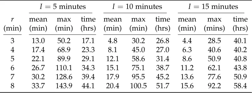
truck finished its transaction; it should be noted that unit of completion timeis in hours whereas the mean and maximum wait times are minutes. These results are averaged over 30 simulation runs for five different tolerance levels (10, 15, 20, 25, and 30 minutes). At each tolerance level, three different interval lengths (5, 10, and 15 minutes) and six different mean transaction times (3, 4, ..., 8 minutes) are provided. The results from these tables indicate that as the mean service time r increases, the truck wait time increases, which is expected. Similarly, as the tolerance level increases, the truck wait time also increases. Again, this is also expected because dispatchers/truckers are willing to go to the seaport terminal even when they expect congestion. The interval length I can be interpreted as the frequency which the dispatchers check the terminal webcam and then make their SEND?(n,t) decisions. As shown in the results, the higher the frequency (i.e. smaller ‘I’ value), the higher the truck wait time. However, because the dispatchers effectively spread out the workload throughout the day the completion timeincreases as I increases.
de-Table 3.3 Mean wait, maximum wait and completiontime for tolerance, L=15 minutes.
I =5 minutes I =10 minutes I =15 minutes
r mean max time mean max time mean max time
(min) (min) (min) (hrs) (min) (min) (hrs) (min) (mins) (hrs)
3 10.0 44.2 17.3 4.8 29.5 26.8 4.4 27.7 40.1
4 13.7 60.1 24.0 7.8 44.0 28.2 6.2 37.8 40.7
5 17.3 77.4 29.8 10.4 57.5 34.7 8.3 49.7 43.2
6 20.9 96.1 35.1 12.8 73.0 42.4 10.2 61.5 49.6
7 24.3 110.9 40.6 14.6 83.2 49.1 11.8 73.4 58.6
8 27.2 122.8 46.0 17.0 94.1 55.4 13.5 81.2 66.6
Table 3.4 Mean wait, maximum wait and completiontime for tolerance, L=20 minutes.
I =5 minutes I =10 minutes I =15 minutes
r mean max time mean max time mean max time
(min) (min) (min) (hrs) (min) (min) (hrs) (min) (mins) (hrs)
3 13.0 50.2 17.1 4.8 30.2 26.8 4.4 28.5 40.1
4 17.4 68.9 23.3 8.1 45.0 27.0 6.3 40.6 40.2
5 22.1 89.9 29.1 12.1 58.6 31.4 8.6 50.9 40.8
6 26.7 110.1 34.3 15.1 75.1 38.7 11.2 62.1 43.8
7 30.2 128.6 39.4 17.9 95.5 45.2 13.6 77.6 50.9
8 33.7 143.9 44.1 20.4 100.5 51.7 15.6 92.2 58.4
Table 3.5 Mean wait, maximum wait and completiontime for tolerance, L=25 minutes.
I =5 minutes I =10 minutes I =15 minutes
r mean max time mean max time mean max time
(min) (min) (min) (hrs) (min) (min) (hrs) (min) (mins) (hrs)
3 15.8 57.4 16.2 4.8 29.8 26.7 4.4 27.3 40.0
4 21.0 78.2 22.7 8.4 44.8 26.8 6.3 40.4 40.0
5 26.6 104.0 28.6 13.6 68.6 29.2 8.6 53.0 40.2
6 31.7 126.2 33.5 17.7 84.5 36.1 12.0 66.2 41.5
7 36.8 143.4 38.6 20.5 95.9 42.4 15.0 82.1 45.9
Table 3.6 Mean wait, maximum wait and completiontime for tolerance, L=30 minutes.
I =5 minutes I =10 minutes I =15 minutes
r mean max time mean max time mean max time
(min) (min) (min) (hrs) (min) (min) (hrs) (min) (mins) (hrs)
3 18.6 62.2 16.1 4.8 30.4 26.7 4.4 29.7 40.0
4 24.8 89.5 22.6 8.2 45.3 26.8 6.2 38.8 40.1
5 31.0 112.1 28.2 15.6 69.6 28.3 8.7 54.7 40.2
6 37.7 136.6 33.4 20.4 88.9 34.9 12.3 64.0 40.7
7 42.8 157.6 38.2 24.1 110.1 41.9 16.5 84.3 43.7 8 47.2 176.7 43.0 27.5 121.4 47.9 19.7 99.1 49.8
Table 3.7 Mean wait, maximum wait and completiontime for tolerance, L=15 minutes (Asynchronous Case).
I =5 minutes I =10 minutes I =15 minutes
r mean max time mean max time mean max time
(min) (min) (min) (hrs) (min) (min) (hrs) (min) (mins) (hrs)
3 8.1 37.1 16.0 3.2 24.9 26.6 3.0 24.8 39.9
4 11.2 50.1 20.9 4.8 37.8 27.7 4.1 33.1 40.9
5 13.4 63.1 25.9 7.5 47.1 31.2 5.4 40.6 42.1
6 15.5 75.0 30.6 9.7 64.4 36.6 7.1 47.9 44.9
7 17.8 87.8 34.8 11.6 73.5 41.0 8.7 59.1 49.8
8 18.1 93.8 41.4 12.7 77.1 48.6 10.0 66.4 58.1
cision making which is more like to be the case in practice. That is, although the terminal operator may update the queuing information every 5 minutes, not all truck dispatchers will make their dispatch decisions immediately after that information is available. It’s more likely that such decisions occur randomly over some interval; in this study, we assume that interval is I.
Figure 3.5 Impact of tolerance on mean wait time of trucks.
levels, L(as shown in Figures 3.5 and 3.6). However, the rate of increase is higher when I is lower. When I = 5 minutes, as the tolerance level increases the truck wait time increases linearly. However, when I = 15 minutes, as the tolerance level increases, there is very little change in truck wait time. It is interesting to note that I nullifies the effect of L.
As explained, the total completion time follows a contrasting pattern. That is, it decreases as the tolerance level increases. Note that when I = 5 minutes, the completiontimeis always lower than when I =10 and 15 minutes, which means that all trucks got served in a short amount of total time. What the completion time results suggest is that when truck dispatchers monitor the webcam more frequently and consequently send trucks to the seaport terminal if the gate is not congested, there is more opportunities for that dispatchers to send trucks; hence, shorter completiontime.
Figure 3.6 Impact of tolerance on maximum wait time of trucks.
tolerance level to demonstrate the convergence characteristics of the truck wait times. Our results show that the convergence does not occur for some scenarios. For instance, if the selected combination of parameters from Table 3.1 impose low demand on the gate (e.g. I = 15 minutes,r= 3 minutes, and L= 15 minutes), all depot agents will use the predictor that predicts a wait time lower than tolerance. Thus, every depot agent ends up sending trucks, but the demand they create at the gate does not exceed the gate capacity; hence, the truck wait timeWx at different intervals xwill never exceed the tolerance level L. Another interesting finding that was observed in our analysis is that when convergence does occur, the mean wait time constantly fluctuates about the tolerance level. This is in contrast to original El Farol Bar problem where the mean attendance converges to the tolerance level (60) after some time. We believe this difference stems from the fact that the gate congestion problem is far more complex than the original problem (see end of section 3.2). Nevertheless, in using nearly the same set of predictive strategies, we were able to show that depot agents could potentially make independent decisions such that they all benefit in the end by having lower total truck wait time. Perhaps, with some modifications of the existing predictors or design some new predictors one could achieve the same convergence characteristic as the original bar problem.
Figure 3.8 Mean wait time of trucks plotted every 15 minutes interval with 15 minutes tolerance.
Figure 3.9 Mean wait time of trucks plotted every 10 minutes interval with 10 minutes tolerance.
A tolerance level of 15 minutes and an interval length of 5 and 10 minutes were selected. The comparison results are shown in Figure 3.10. These results show that our model yields 43% and 63% lower mean wait time for an interval of 5 and 10 minutes, respectively. Similarly, the reduction in maximum wait time is 22% and 40%, respectively. However, the total completion time is higher, by about 18% and 40% for the two intervals, respectively.
r Mean Max Completion time (mins) (mins) (mins) (hrs)
5 26.6 86.4 12.8
Figure 3.10 Results showing wait time and completion time with and without using predictive strategies.
Table 3.8 Percentage decrease in emission.
Pollutant I =5,L =15 I =10,L=15
HC 2.30% 3.40%
CO 2.40% 3.50%
NOx 1.70% 2.40%
PM10 1.50% 2.20%
PM25 1.50% 2.20%
CO2 1.60% 2.30%
The shown distribution of truck wait times from our simulation model matches that of empirical data collected from actual terminals. The results from Figure 3.11 highlight the extent of the marine terminal gate congestion problem. As shown, a good portion of the trucks spend more than 10 minutes queuing (i.e. idling and stop-and-go lugging) at the gate. This represents a serious environmental issue. Emissions from diesel engines of drayage trucks can cause a critical share of local and regional particulate matter (PM 2.5), nitrogen oxides (NOx) and greenhouse gas (GHG) emissions. Also, according to the EPA, PM 2.5 emissions from diesel engines are a serious health concern. Thus, reducing the average inbound gate queueing time will likely lead to a reduction in emissions as well as fuel and cost savings for trucks. To quantify the benefit in terms of emissions reduction using our proposed paradigm to manage gate congestion, a simple emissions analysis was performed. Table 3.8 summarizes the comparative results found using the SmartWay DrayFLEET model, developed by EPA in collaboration with the Federal Highway Administration. The results in Table 3.8 correspond to a dispatch rate of 6 trucks/depot/hr and mean transaction time of 5 minutes.
3.7 Conclusions andFutureWork
Though some remedial measures are employed, their benefits are still largely unknown and published research is very limited. To this end, this paper presents an agent-based approach where depots can manage (without any collaboration with one another) to minimize congestion at seaport terminal gates by using the provided real-time gate congestion information and some simple logic for estimating the expected truck wait time.
Our work is inspired by the well known El Farol Bar problem, but we have modified the methodology and implementation to account for the additional com-plexity and dynamics involved with truck dispatch and queuing at terminal gates. Our simulation model implementation contains a handful of parameters that at-tempts to capture all the variables that are relevant to the gate congestion problem. Extensive experiments were conducted by using practical ranges of the parameters. The results demonstrate that the depots can effectively and successfully minimize truck wait time at the terminal gate by adopting our proposed framework by distributing the demand more uniformly over the operational hours (i.e. adopt a higher I). Our findings also reveal how the selection of different parameters in our model will impact the average and maximum wait time of trucks, as well as how depots can benefit from extended operational hours. Results from our simple emissions analysis show that a good amount of emissions reduction can be gained over the base case (do nothing) scenario.
a dispatcher to have 12 or more predictive strategies. Another interesting line of research would be to incorporate more sophisticated learning models to determine if they would improve the overall system performance.