Solving Discontinuous Collocation Equations for a Class of Brain Tumor Models on GPUs

Solving Discontinuous Collocation Equations for a

Class of Brain Tumor Models on GPUs

I.E. Athanasakis, N.D. Vilanakis and E.N. Mathioudakis

Abstract—Brain tumor modeling has been a challenging research subject over the past decades. Incorporation of brain’s tissue heterogeneity (gray-white matter) in the models, has been realized by the introduction of a discontinuous diffusion coefficient in the core PDE, as tumor cells migrate with different rates in brain’s white and gray matter. For the numerical treatment of these models, recently, a fourth order Discontinuous Hermite Collocation (DHC) method coupled with high order semi implicit and strongly stable Runge-Kutta (RK) time discretization schemes, has been successfully developed. And as, at each time step, large linear systems has to be solved, significant computational cost emerges. For their ef-ficient solution the incomplete LU factorization preconditioned BiCG stabilized iterative method, suggested by the eigenvalue topology, is adopted. The implementation of the numerical method in Matlab environment takes place in a multicore CPU-only computational architecture. Here, we present the design and development of a CPU-GPU parallel algorithm to carry out the whole computation. Its mapping and implementation on a GPU-CPU architecture necessitates the use of CUDA development tools. Several numerical experiments are presented to demonstrate the efficiency of the parallel algorithm.

Index Terms—Discontinuous Hermite Collocation, DIRK methods, Matlab, CUDA, CPU-GPU computations.

I. THE NUMERICAL BRAIN TUMOR MODEL

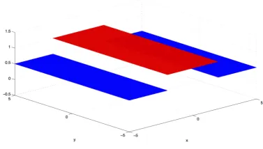
Simulations of the progress of untreated diffusive brain tumors are based on classical reaction-diffusion mathemat-ical models, such as in [1],[2] and [3]. Recently, Swanson ([4],[5]) introduced an appropriately discontinuous diffusion coefficient and generalized these models incorporating the heterogeneity of the brain tissue (white-grey matter). The basic linear version of the model is then expressed with the following reaction-diffusion equation:

Fig. 1. Discontinuous coefficientDfor a two-value problem.

Manuscript received March 23, 2015 ; revised April 6, 2015.

This work was supported by EU (European Social Fund ESF) and Greek funds through the operational programEducation and Lifelong Learningof the National Strategic Reference Framework (NSRF) - Research Funding Program: THALIS.

All authors are with the Applied Mathematics and Computers Laboratory, Technical University of Crete, University Campus, 73132 Chania, Crete, Greece – Corresponding author’s e-mail: [email protected].

∂c¯

∂¯t =∇ ·

¯

D(¯x)∇¯c

+ρc ,¯ (1)

where¯c(¯x,¯t)denotes the tumour cell density,ρdenotes the net proliferation rate, and D¯(¯x) is the diffusion coefficient representing the active motility of malignant cells satisfying

¯

D(¯x) =

Dg , ¯x in Grey Matter

Dw , ¯x in White Matter

, (2)

withDg and Dw scalars andDw > Dg. Using the

dimen-sionless variables :

x= r _ρ

Dw

¯

x , t=ρ¯t , f(x) = ¯f

r _ρ

Dw

¯ x

,

and c(x, t) = ¯c

r _ρ

Dw

¯ x, ρt¯

_D

w

ρN0

withN0=Rf(x)dx to denote the initial number of tumour

cells in the brain att= 0, as well as the transformation

c(x, t) =etu(x, t) ,

the model in2 + 1dimensions reduces to

 



ut= (Dux)x+ (Duy)y , (x, y, t)∈[a, b]2×R+

∂u

∂η = 0, u(x, y,0) =f(x, y), D=

γ, x /∈[w1, w2)

1, x∈[w1, w2)

(3) where the diffusion coefficientD is discontinuous along two interface lines x = w1 and x = w2, as it is depicted in

Fig. 1. The discontinuous diffusion coefficient D, directly implies discontinuity ofux, hence continuity ofDux, across

each interface line. In fact, the linear parabolic nature of the initial-boundary value problem implies continuity ofuacross each interface, that is

[u] := lim

x→w_k+

u(x, y0)− lim

x→w−_k

u(x, y0) = 0 (4)

and

[Dux] := lim x→w+_k

Dux(x, y0)− lim

x→w−_k

Dux(x, y0) = 0 (5)

wherek= 1,2andy=y0 is a fixed point in[a, b]. Taking,

now, into consideration the above two continuity constrains an alternative way to state the model can be described by

 



ut=Duxx+Duyy , (x, y)∈R`

∂u

∂η = 0 , u(x, y,0) =f(x, y)

[u] = 0 , [Dux] = 0 at x=w1,2

(6)

whereR1:= [a, w1)×[a, b] , R2:= [w1, w2)×[a, b]and

R3:= [w1, b)×[a, b].

high order Runge-Kutta schemes for the effective solution of the model problem described above. The approximate solution, DHC method seeks, is in the form

U(x, y, t) =

2Ny+2

X

i=1

2Nx+2

X

j=1

[αi,j(t)φi(x)φj(y)] (7)

whereNy =Nx=Nx1+Nx2+Nx3 denotes the number of

subintervals ofR` andφthe Hermite cubic basis functions.

For the determination of theαi,j unknowns in (7), the DHC

leads to the system of ODEs (cf. [6]):

C_x0⊗C_y0a˙ = DxCx2⊗C

0

y

a+ DxCx0⊗C

2

y

a (8)

whereC_x∗andC_y∗denote the1dDiscontinuous and Continu-ous Collocation matrices respectively (cf. [7]), Dxis the

di-agonal matrix Dx =diag(γ, . . . , γ,1, . . . ,1, γ, . . . , γ), and ⊗ denotes the Kronecker (tensor) matrix product. Setting, now, A0:=Cx0⊗Cy0 andB:=DxCx2⊗Cy0+DxCx0⊗Cy2

of order N= 4NxNy equation (8) can be written as:

A0a˙ =Ba or a˙ =C(t,a) for C(t,a) =A−01Ba. (9)

Finally, the DHC method is coupled (cf. [7],[6]) with an optimal two-step and third-order Diagonally implicit Runge-Kutta scheme [8] for the time discretization, yielding the system of linear equations:

a(n,1)=a(n)+τ λ C(tn,1,a(n,1))

a(n,2)=a(n)+τh(1−2λ)C(tn,1,a(n,1)) +λC(tn,2,a(n,2))

i

a(n+1)=a(n)+τ 2

h

C(tn,1,a(n,1)) +C(tn,2,a(n,2))

i (10)

or, equivalently,

A a(n,1)=A0 a(n)

A a(n,2)=A0 a(n)+τ(1−2λ)B a(n,1) .

A0 a(n+1)=A0 a(n)+

τ

2 [B a

(n,1)_+B

a(n,2)] (11)

whereA:=A0−τ λB,τis the time spacing andλ= 1₂+

√

3

2 .

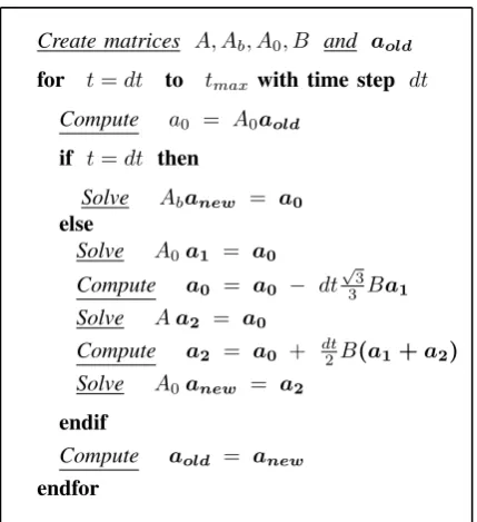
The solution, now, of the above system of linear equations is computationally described by means of the following algorithm:

Create matrices A, Ab, A0, B and aold

for t=dt to tmax with time step dt

Compute a0 = A0aold

if t=dt then

Solve Abanew = a0

else

Solve A0a1 = a0

Compute a0 = a0 − dt

√

3

3 Ba1

Solve Aa2 = a0

Compute a2 = a0 + dt₂B(a1+a2)

Solve A0anew = a2

endif

Compute aold = anew

endfor

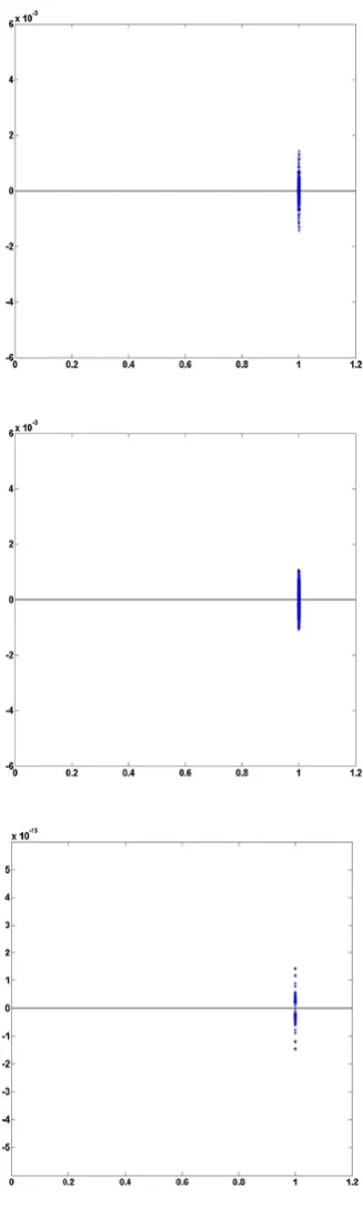
Fig. 3. Eigenvalue charts of matricesAb, A0 and A, respctively,

with the application of the preconditioning technique.

We remark that the first step of the algorithm utilizes the matrix Ab, where Ab := A0−τ B. The use of this matrix

refers to the application of Backward Euler method to avoid possible oscillations. For every other step from there on, matrices A, A0 and B involved in the calculations, arise

from the DIRK scheme. And as all of them are large and sparse, iterative methods are preferable for the solution of the corresponding linear systems. The iterative method could be a stationary one or a Krylov subspace method. A stationary method would demand a matrix splitting in the form of

A = D−L−U, but the nature and the properties of the matrices indicate that would not be an appropriate approach. On the other hand, Krylov subspace methods, where matrix-vector products are the dominant operations, are well suited for parallel execution. Therefore, the BiCGSTAB method [9] is preferred for the solution of the three linear systems in each step of the algorithm. The selection of this particular method is justified by the eigenvalue properties of the matrices involved in the linear systems described above, as well as effective preconditioning techniques.

To be more specific, calculation of the eigenvalues (see Fig. 2) indicates that a suitable preconditioning technique would have a positive effect on the convergence rate of the Krylov iterative method. Since the matrices are stored in a sparse format, the incomplete LU factorization of each matrix Ab, A0 and A, that is MAb :=iLU(Ab),

MA0 :=iLU(A0) andMA:=iLU(A), is a very convenient

choice as a preconditioner. An essential fact we should emphasize on, is that all three matrices are time independent, therefore their iLU factorization computation is performed once before the time stepping process.

Following, now, iLU(A) preconditioning, it becomes clear (inspect Fig. 3) that the eigenvalues of each one of the matrices are clustered around unity and notably close to the real semi-axis, indicating the proper selection of the preconditioning technique and encouraging the use of the BiCGSTAB method instead of GMRES [10].

II. THE PARALLEL ALGORITHM

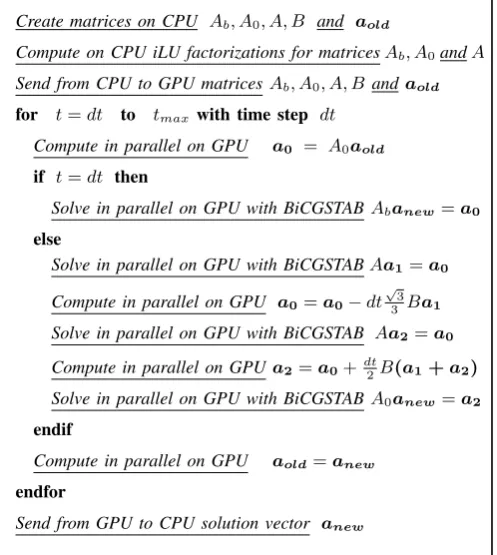
During each time step, the proposed numerical scheme requires the solution of three linear systems, with time-independent coefficient matrices, by an iterative method (BiCGSTAB) in which basic linear algebra operations dom-inate. The decoding of this sentence indicates the develop-ment of an application that will utilize both the CPU and the GPU; sequential parts, like backward and forward substitu-tions, will be executed on the CPU, while the demanding floating-point operations of the compute-intensive parts will be transferred and performed on the GPU. It should be recalled that a Graphics Processing Unit possesses a great number of cores which are heavily multithreaded, working in a single instruction-multiple data mode. That makes it an excellent numeric computing engine, in case of matrix-vector multiplication operations (see for instance [11] and [12]). Therefore, in the parallel algorithm the creation of the matricesAb, A0,A,B and vectoraold along with the

computation of the iLU factorization of each matrix take place on the CPU. The data are being copied to the GPU’s memory before the beginning of the time stepping process and from there on the vast majority of the floating-point operations is performed on the GPU. The communication cost is related to the length of the vectors needed to be transferred between CPU and GPU for the execution of the preconditioned system’s backward and forward substitutions with coefficient matricesMAb,MA0 andMA.

Create matrices on CPU Ab, A0, A, B and aold

Compute on CPU iLU factorizations for matricesAb, A0andA Send from CPU to GPU matricesAb, A0, A, B andaold

for t=dt to tmaxwith time step dt

Compute in parallel on GPU a0 = A0aold

if t=dt then

Solve in parallel on GPU with BiCGSTABAbanew=a0 else

Solve in parallel on GPU with BiCGSTABAa1=a0

Compute in parallel on GPU a0=a0−dt √

3 3 Ba1 Solve in parallel on GPU with BiCGSTAB Aa2=a0

Compute in parallel on GPUa2=a0+dt₂B(a1+a2)

Solve in parallel on GPU with BiCGSTABA0anew=a2

endif

Compute in parallel on GPU aold=anew

endfor

Send from GPU to CPU solution vector anew

The iLU preconditioned GPU - BiCGSTAB iterative method is described with the following parallel algorithm in case of solving the Ax=blinear system, withLU been the incomplete factorization of matrixA :

Choose initial approximationx(0)_{of the solutionx} Compute on GPU r(0) = b−Ax(0)

Chooserˆ(usuallyˆr = r(0)₎

fori = 1,2, ...

Compute on GPU ρi−1 = ˆrTr(i−1)

ifρi−1 = 0 method fails

if i = 1

Compute on GPU p(1) = r(0)

else

βi−1 =

ρi−1

ρi−2

αi−1

ωi−1

Compute on GPUp(i)_=r(i−1)_+β

i−1(p(i−1)− ωi−1v(i−1))

endif

Send from GPU to CPU p(i) Solve on CPU Ly = p(i) Solve on CPU Upˆ= y

Send from CPU to GPU pˆ

Compute on GPU v(i) = Apˆ

Compute on GPU αi =

ρi−1 ˆ

rTv(i) Compute on GPU s = r(i−1) _{− α}

iv(i) if ksk is small enoughthen

Compute on GPU x(i) = x(i−1) + αipˆ stop

Send from GPU to CPU s

Solve on CPU Ly = s Solve on CPU U z = y

Send from CPU to GPU z

Compute on GPU t = A z

−5 −4 −3 −2 −1 0 1 2 3 4 5 −5 0 5 0 0.05 0.1 0.15 0.2 0.25 0.3 0.35 0.4 0.45 0.5 t= 1 −5 −4 −3 −2 −1 0 1 2 3 4 5 −5 −4 −3 −2 −1 0 1 2 3 4 5 0 0.05 0.1 0.15 0.2 0.25 0.3 0.35 0.4 0.45 0.5 t= 2 −5 −4 −3 −2 −1 0 1 2 3 4 5 −5 −4 −3 −2 −1 0 1 2 3 4 5 0 0.05 0.1 0.15 0.2 0.25 0.3 0.35 0.4 0.45 0.5 t= 3 −5 −4 −3 −2 −1 0 1 2 3 4 5 −5 −4 −3 −2 −1 0 1 2 3 4 5 0 0.05 0.1 0.15 0.2 0.25 0.3 0.35 0.4 0.45 0.5 t= 4

−5 −4 −3 −2 −1 0 1 2 3 4 5 −5

−4 −3 −2 −1 0 1 2 3 4 5

0.01 0.02 0.03 0.04 0.05 0.06

−5 −4 −3 −2 −1 0 1 2 3 4 5 −5

−4 −3 −2 −1 0 1 2 3 4 5

0.01 0.02 0.03 0.04 0.05 0.06 0.07 0.08 0.09

−5 −4 −3 −2 −1 0 1 2 3 4 5 −5

−4 −3 −2 −1 0 1 2 3 4 5

0.02 0.04 0.06 0.08 0.1 0.12 0.14 0.16 0.18

−5 −4 −3 −2 −1 0 1 2 3 4 5 −5

−4 −3 −2 −1 0 1 2 3 4 5

0.05 0.1 0.15 0.2 0.25 0.3 0.35 0.4

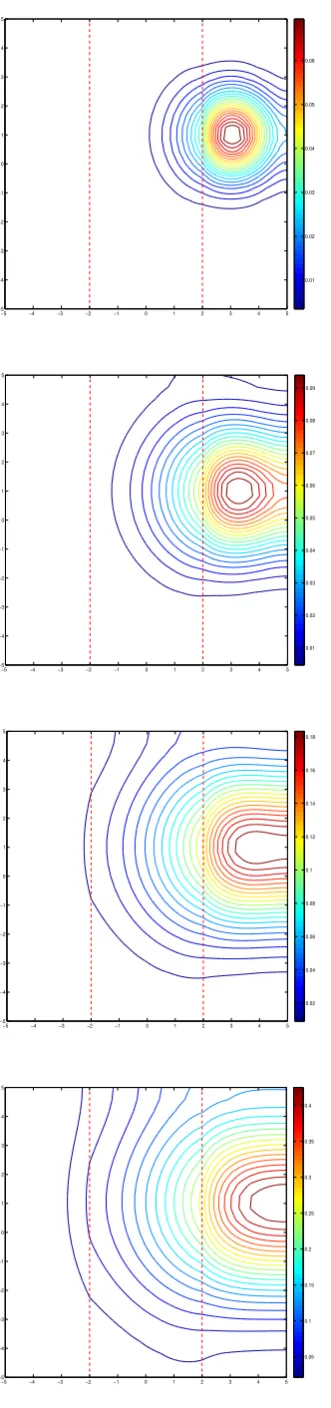
Fig. 5. Model problem’s contour plots of approximate solutions at time stepst= 1,2,3and 4 respectively.

.

Compute on GPU ωi = s

T_t tTt

Compute on GPU x(i) _{= x}(i−1) _{+ α}

ipˆ + ωiz Check for Convergence

if ωi = 0 stop

Compute on GPU r(i) _{= s − ω}

it endfor

III. CPU-GPUIMPLEMENTATION

The implementations of the developed algorithm were carried out on a shared memory HP SL390s G7, consisting of two 6-core Xeon [email protected] GHz type processors with 12 MB Level 3 cache memory each. The total memory is 24 GB and the operating system is Oracle’s Linux version 6.2. The machine is also equipped with a Fermi edition Tesla M2070 GPU, with 6 GB of memory and 448 cores on 14 multiprocessors. The time measurements comparison is between 2 different applications that were developed. The first one was developed in Matlab R2014b [13] and runs on a multicore CPU-only environment, while the second one was developed in Matlab R2014b and in PGI’s 15.3 CUDA Fortran [14] and runs on a CPU-GPU environment. In the development of the CPU-GPU application, subroutines from cuBLAS and cuSPARSE libraries [15] (in GPU operations) and from SparseKit (in CPU operations) were used for CUDA 6.0 compiler suite [16]. We have to mention that Matlab software does not support yet GPU computations for sparse matrices. This is the main reason that the CPU-GPU part of the algorithm is implemented in CUDA Fortran. The Matlab Compiler toolbox from 2014b software version is used for the compilation of the standalone multicore Matlab application for the CPU-only implementations.

Time evolution of the brain’s tumor model numerical solution is depicted in Figures Fig. 4 and 5, for the case of tmax = 4 and dt = 0.05, and the numerical scheme’s successful treatment of the problem is being demonstrated. The regions (stripes) with different rates of cell motility as well as the discontinuity interfaces are visible and handled effectively by the numerical scheme.

In the following Table I the time measurements (in seconds) are presented, comparing the Matlab multithread CPU implementation and the CUDA Fortran CPU-GPU implementation, in different cases of discretization, namely n =400, 1600, 6400 and 25600 finite elements. The size of the linear systems involved in each test case is equal to the number of unknowns N = 4n to be evaluated. Also the total degrees of freedom (dof) are mentioned for every finite element problem size. The observed acceleration is graphically presented in Fig. 6 for all test cases between the multicore CPU Matlab and the CPU-GPU Matlab-CUDA Fortran realization of the parallel algorithm.

Table I :Execution time measurements for Matlab multithread CPU and Matlab-CUDA Fortran CPU-GPU implementations Number of Number of CPU Matlab CPU - GPU

elements unknowns dof Time Time

400 1600 6400 0.83 0.31

1600 6400 25600 2.35 0.94

6400 25600 102400 11.5 4.55

25600 102400 409600 202 81.8

Fig. 6. Speedup measurements for CPU Matlab and CPU-GPU Matlab-CUDA Fortran implementations.

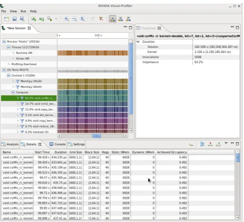
time, while the vector addition operation which was performed 13450 times consumed 11%.

Fig. 7. NVIDIA’s Visual Profiler graphical performance application tool.

The above observations were made using the NVIDIA’s Visual Profiler as shown in Fig. 7.

IV. CONCLUSIONS

A new parallel algorithm for computing architectures with ac-celerators, implementing the Discontinuous Hermite Collocation method, has been developed. The algorithm was realized on ma-chines with Graphics Processing Units and the time measurements were compared to Matlab multicore implementations. The results reveal the highest efficiency of the CPU-GPU implementation since the performance acceleration that was observed reached 2.5x.

ACKNOWLEDGMENT

The present research work has been co-financed by the European Union (European Social Fund ESF) and Greek national funds through the Operational ProgramEducation and Lifelong Learning

of the National Strategic Reference Framework (NSRF) - Research Funding Program: THALIS. Investing in knowledge society through the European Social Fund.

REFERENCES

[1] G.C. Cruywagen, D.E. Woodward, P. Tracqui, G.T. Bartoo, J.D. Murray and E.C. Alvord Jr., “The modeling of diffusive tumours, journal of biological systems,”Journal of Biological Systems, vol. 3, pp. 937–945, 1995.

[2] P.K. Burgess, P.M. Kulesa, J.D. Murray and E.C. Alvord Jr., “The inter-action of growth rates and diffusion coefficients in a three-dimensional mathematical model of gliomas,” Journal of Neuropathology and Experimental Neurology, vol. 14(5), pp. 704–713, 1997.

[3] D.E. Woodward, J.Cook, P.Tracqui, G.C. Cruywagen, J.D. Murray and E.C. Alvord Jr., “A mathematical model of glioma growth: the effect of extent of surgical resection, journal of biological systems,”Cell Proliferation, vol. 29, pp. 269–288, 1996.

[4] K.R. Swanson, E.C. Alvord Jr. and J.D. Murray, “A quantitive model for differential motility of gliomas in grey and white matter,”Cell Proliferation, vol. 33, pp. 317–329, 2000.

[5] K. R. Swanson, C. Bridge, J. D. Murray and E. C. Alvord Jr., “Virtual and real brain tumours:using mathematical modeling to quantify glioma growth and invasion,”J.Neurol.Sci, vol. 216, pp. 1–10, 2003. [6] I.E. Athanasakis, E.P. Papadopoulou and Y.G. Saridakis,

“Discon-tinuous Tensor Product Collocation and Runge-Kutta schemes for heterogeneous brain tumor invasion models,”Submitted, 2015. [7] I.E. Athanasakis, M.G. Papadomanolaki, E.P. Papadopoulou and Y.G.

Saridakis, “Discontinuous Hermite Collocation and Diagonally Im-plicit RK3 for a brain tumour invasion model,”Proceedings of WCE 2013 Vol I, IAENG, pp. 241–246, 2013.

[8] R. Alexander, “Diagonally implicit runge-kutta methods for stiff odes,” SIAM Num. Anal., vol. 14(5), pp. 1006–1021, 1977.

[9] H.A. van der Vorst, “Bi-CGSTAB : A fast and smoothly converging variant of bi-cg for the solution of nonsymmetric linear systems,”SIAM J. Sci.Stat.Comp., vol. 13, pp. 631–644, 1992.

[10] Y. Saad,Iterative methods for sparse linear systems. SIAM, 2003. [11] E.N. Mathioudakis, N.D. Vilanakis, E.P. Papadopoulou and Y.G.

Sari-dakis, “Parallel iterative solution of the hermite collocation equations on GPUs,”Proceedings of WCE 2013 Vol II, IAENG, pp. 1281–1286, 2013.

[12] N.D. Vilanakis and E.N. Mathioudakis, “Parallel iterative solution of the hermite collocation equations on GPUs II,”Journal of Physics: Conference Series, vol. 490(1), 2014.

[13] http://www.mathworks.com. [14] http://www.pgroup.com. [15] http://www.nvidia.com/cuda.