Parameter Selection and Verification Techniques Based on Global
Sensitivity Analysis Illustrated for an HIV Model
Mami T. Wentworth, Ralph C. Smith and H.T. Banks
Department of Mathematics
Center for Research in Scientific Computation
North Carolina State University
Raleigh, NC 27695
February 11, 2015
Abstract
We consider parameter selection and verification techniques for models having one or more parameters that are noninfluential in the sense that they minimally impact model outputs. We illustrate these techniques for a dynamic HIV model but note that the parameter selection and verification framework is applicable to a wide range of biological and physical models. To accommodate the nonlinear input to output relations, which are typical for such models, we focus on global sensitivity analysis techniques, including those based on partial correlations, Sobol indices based on second-order model representations, and Morris indices, as well as a parameter selection technique based on standard errors. A significant objective is to provide verification strategies to assess the accuracy of those techniques, which we illustrate in the context of the HIV model.
1
Introduction
Biological and physical models commonly have tens to hundreds of inputs – comprised of parameters, dis-cretized spatially-varying coefficients, initial or boundary conditions, or exogenous forces – many of which have minimal influence on model responses. This necessitates the development of robust analysis techniques to establish subsets or subspaces of influential parameters or inputs. This challenge is exacerbated for models such as neutronics equations, which can have 106inputs, of which only 50-100 are considered influential. The need for robust parameter selection techniques is further motivated by the following objectives: (i) determine those inputs that can be uniquely estimated from measured data; (ii) establish the robustness or fragility of models with respect to certain parameter sets; (iii) simplify models by fixing insensitive inputs; and (iv) guide experimental design by ascertaining parameter subsets or subspaces that have the greatest impact on parameter or response sensitivity.
To establish notation and terminology, we consider the nonlinear input-output relation
y=f(q)
where q= [q1, . . . , qp] denotes the model inputs – e.g., parameters, initial or boundary conditions – and f denotes the mathematical model. For this discussion, we consider real-valued responsesy∈R1.
A significant goal of input or parameter selection techniques is to establish subsets or subspaces of inputs or parameters that can be uniquely identified from data or that strongly influence model responses. Such subsets can be characterized by the concepts of identifiable and influential parameter sets.
q
y
q
y
q
y
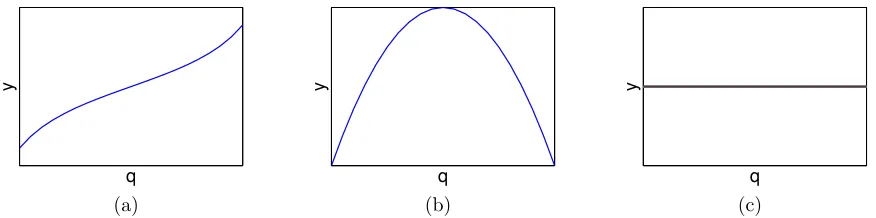
(a) (b) (c)
Figure 1: Illustration ofy=f(q) for (a) identifiable, (b) unidentifiable and (c) noninfluential parametersq.
Hence identifiable parameters can be uniquely determined from observations. An example of identifiable and nonidentifiable parameters are illustrated in Figure 1 (a) and (b).
Influential parameter spaces are sometimes defined differently in various disciplines. We define the param-eter setq= [q1, . . . , qp] to benoninfluentialon the spaceN I(q) iff(q)−f(q∗)< εfor allqandq∗∈ N I(q). The spaceI(q) of influential parameters is defined to be the orthogonal component ofN I(q). Noninfluential parameters, like nonidentifiable parameters, can be fixed for model calibration and uncertainty propagation. Hence, the space of noninfluential parameters is a subspace of the space of nonidentifiable parameters. An example of a noninfluential parameter is illustrated in Figure 1 (c). Furthermore, parameter q1 is more influential than parameterq2if changes inq1affect greater changes iny than changes inq2do. See Figure 2 for an example of highly and minimally influential parameters. We will quantify the degree of influence using global sensitivity analysis.
For linearly parameterized problems y = Aq, it is shown in Chapter 6 of [20] that deterministic and parametrized QR or SVD algorithms can be used to determine subspaces of influential parameters. For the nonlinearly parametrized problems, one typically resorts to global sensitivity analysis or active subspace techniques.
In this paper, we focus on global sensitivity analysis and subset selection based on standard errors to determine subsetsqs={qs
1, . . . , qsp˜} ⊂q={q1, . . . , qp}of influential parameters. This differs from subspace selection techniques – typically based on QR or SVD algorithms with inputs randomly selected from the admissible input space – which can include linear combinations of inputs [2, 11, 20]. The comparison of active input subspaces with the subset established here for the HIV model constitutes future research.
a b
q 1
a b
q 2
(a) (b)
Figure 2: Illustration of influential parameters whereq1 is more influential than q2.
1.1
HIV Model, Inputs and Responses
˙
T1=−d1T1−(1−ξ1(t))k1VIT1−γTT1+pT
a
TVI
VI+KV +aA
T2
˙
T1∗= (1−ξ1(t))k1VIT1−δT1∗−mE1T1∗−γTT1∗+pT
a
TVI
VI+KV +aA
T2∗
˙
T2=λT
Ks
VI+Ks
−γTT1−d2T2−(1−f ξ1(t))k2VIT2−
aTVI
VI+KV +aA
T2
˙
T2∗=γTT1∗+ (1−f ξ1(t))k2VIT2−d2T2∗−
a
TVI
VI+KV +aA
T2∗
˙
VI = (1−ξ2(t))103NTδT1∗−cVI−103[(1−ξ1(t))ρ1k1T1+ (1−f ξ1(t))ρ2k2T2]VI ˙
VN I=ξ2(t)103NTδT1∗−cVN I ˙
E1=λE+
bE1T ∗ 1
T1∗+Kb1
E1−
dET1∗
T1∗+Kd
E1−δE1E1−γE
T1+T1∗
T1+T1∗+Kγ
E1+
pEaEVI
VI+KV
E2
˙
E2=γE
T1+T1∗
T1+T1∗+Kγ
E1+
bE2Kb2
E2+Kb2
E2−δE2E2−
aEVI
VI+KV
E2
(1)
with initial conditions [T1(0), T1∗(0), T2(0), T2∗(0), VI(0), VN I(0), E1(0), E2(0)]. Here,T1 and T1∗ respectively denote uninfected and infected activated (antigen-specific) CD4+ T-cells. Uninfected resting, i.e., not acti-vated, CD4+ T-cells are denoted byT2and infected resting CD4+ T-cells are denoted byT2∗. Infectious free virus is denoted byVI; this is the virus that is capable of infecting other cells in the plasma. On the other hand,VN I denotes non-infectious free virus, which is yielded inactive by protease inhibitors. HIV-specific effector CD8+ T-cells are denoted by E1 and HIV-specific memory CD8+ T-cells are denoted by E2. The compartments of the model are depicted in Figure 3.
Several terms in the model (1) are based on the law of mass action, so that the rate of change in population size is proportional to the population size. The terms−d1T1 and γTT1 in ˙T1 are examples of mass action terms. Other terms are based on Michaelis-Menten kinetics, in which the rate saturates at a maximum. An example of this type is aTVI
VI+KV, which is the activation of infected HIV specific resting CD4+ T-cells
with aT being the maximum activation rate. The term VλTKS
I+KS in the differential equation for ˙T
∗
2 accounts for the source rate of naive CD4+ T-cells. In the equation for ˙E1, bE1T1∗
T∗
1+Kb1E1 and − dET1∗ T∗
1+KdE1 respectively
represent dynamic effects that activated, infected CD4+ T-cells have on the effector CD8+ T-cells when
Parameter Explanation
δ Viral produced lysis rate ofT1∗ d2 T2andT2∗ natural death rate
δE2 Death rate ofE2
m Rate of removal by cell lysis ofT1∗ from the system byE1
γT Rate at whichT1andT1∗ differentiate intoT2 andT2∗ , respectively
c Natural clearance rate ofVI andVN I
δE1 Constant death rate ofE1
γE Source term forE1
k2 Production rate ofT2∗ due to encounters betweenT2andVI that is less thank1
ρ1 Rate of removal ofVII through successful infection ofT1
ρ2 Rate of removal ofVI through successful infection of T2
d1 Natural death rate ofT1
2 Relative effectiveness of protease inhibitor (PI)
aA Activation rate ofT2and∗2 by non-HIV antigen
1 Relative effectiveness of reverse transcriptase inhibitor (RTI)
pT Net proliferation ofT1andT1∗ due to clonal expansion and programmed contraction
pE Net proliferation ofE1 due to clonal expansion and programmed contraction
k1 Production rate ofT1∗ from encounters between T1andVI
NT Number of RNA copies produced during the process ofT1∗ lysis
aT Maximum activation rate ofT2 andT2∗
f Efficacy of treatment 0≤f ≤1
λE Constant differentiation ofE2 intoE1
KV Half-saturation constant of virus
Table 1: Description of parameters in the model (1).
Kb1 < Kd and bE1 < bE. Also in this differential equation, pVEI+KaEVVIE2 represents the activation of memory
CD8+ T-cells into effector CD8+ T-cells. In the differential equation for ˙E2, E1(T1+T1∗)
T1+T1∗+Kγ has an essential role
that activated CD4+ T-cells play in the generation of memory CD8+ T-cells, whereas bE2Kb2E2
E2+Kb2 andδE2E2 are homeostatic regulation terms inE2.
The parameters in the HIV model (1) are described in Table 1 and nominal values for parameters and initial conditions reported in [3] are compiled in Table 2. The functionsξ1=1u(t) andξ2=2u(t) represent the impact of the treatment. Here,1is the effectiveness of the reverse transcriptase inhibitor (RTI), whereas
2 is the effectiveness of the protease inhibitor (PI). Also, u(t) is the HAART drug level, where u(t) = 1 when the patient is on treatment, and u(t) = 0 when the patient is off treatment. Parameters such as 1 and2, along with many others, can not be directly measured and hence must be estimated through a fit to data.
Among these parameters, however, some do not influence model outputs. These parameters must be identified via parameter selection prior to parameter estimation. Isolating these noninfluential parameters allows us to reduce the parameter dimensions for model calibration and focus on estimating those parameters that can be uniquely determined from the data.
Based on results from [3], we focus on the 15 parameters and initial conditions
q= [λT, d1, 1, k1, aT, 2, NT, bE2, aE, pE, aA, pT, T1(0), T1∗(0), T2(0)] (2)
whose values tend to be patient specific. Here, the input dimensions is p = 15. The associated random variable, considered for global sensitivity analysis, is denoted byQ. Also, we denoted the admissible input space of biologically feasible parameters and initial conditions byQ. The lower and upper bounds for each
parameter, whereqi ∈ [`bi, ubi], is summarized in Table 3. For more details of the terms and parameters, see [3, 5].
λT = 3.2543 d1 = 0.1317 1 = 0.5241 k1 = 4.8200e-5
aT = 2.3198e-4 2 = 0.7149 NT = 79.26 bE2 = 0.34554
aE = 1.5332e-2 pE = 1.0294 aA= 8.07e-5 pT = 5.531
γT = 3.792e-4 d2 = 3.096e-3 f = 0.5068 k2 = 2.005e-9
δ= 0.2095 m= 1.127e-3 c= 5.818 λE = 9.9930e-4
bE1= 3.885e-2 Kb1 = 2.488e-2 dE = 6.278e-2 Kd = 0.12
δE1= 5.967e-2 Kb2 = 86.97 γE = 5.154e-4 Kγ = 1.357
KV = 14.79 δE2 = 1.450e-3 Ks = 2.789e+4 T1(0) = 12.135
T1∗(0) = 5.8604e-4 T2(0) = 823.59 T2∗(0) = 7.521e-3 VI(0)= 3.571e+3
VN I(0) = 3.571e+3 E1(0) = 6.821e-2 E2(0) = 0.6909
Table 2: Nominal values of parameters and initial conditions from [3].
T1∗+T2+T2∗) as well as total RNA copies/mL-plasma (VI+VN I) were recorded during this process. For global sensitivity analysis, we require a scaler response. At the same time, we are interested in how parameters affect the model output for the feasible input as well for the entire duration of therapy. For these reasons, we choose our scalar model response to be
f(q) =
Z 1500
0
T1(t;q) +T1∗(t;q) +T2(t;q) +T2∗(t;q)dt+
Z 1500
0
VI(t;q) +VN I(t;q)dt.
To test the parameter selection techniques, we generate synthetic data using the mean values from the model calibration performed in [5], which are summarized in Table 2. The model is solved numerically using
ode15sin MATLAB.
1.2
Previous Work and Paper Organization
Whereas global sensitivity analysis techniques for parameter selection have not previously been investigated for this dynamic HIV model, certain techniques have been used to analyze other biological models.
Readers are referred to [10] for a case study illustrating the use of sensitivity analysis for a rice model, and [13, 23] for examples of parameter selection in computational and systems biology. The subset selection developed in [4, 6, 9] is applied to the HIV model (1) in [3] and we compare our sensitivity-based parameter subsets to those of [3] in Section 4.
In Section 2, we illustrate the difference between local and global sensitivity analysis using a simple portfolio model. In Section 3, we discuss four different techniques for parameter selection. We start with Partial Correlation [1], which quantifies the linear effects of parameters on the model response. Secondly, we discuss Sobol indices, which are variance-based methods based on a second-order Sobol decomposition. For the HIV example, we discuss the limited accuracy of this decomposition and its affect on parameter selection. Thirdly, we summarize Morris indices using a screening method that ranks parameters in the order of importance. Finally, we discuss the parameter subset selection algorithm discussed in [3]. In Section 4, we present our results of applying parameter selection techniques to the HIV model. We interpret the sensitivity indices from each method and provide a comparison for identifying influential parameters. We present verification techniques to illustrate that non-influential parameters should not affect the model
λT d1 1 k1 aT 2 NT bE2
`bi 3.1 0.11 0.43 4.0e-5 2.0e-4 0.63 65 0.28
ubi 3.5 0.15 0.6 5.5e-5 2.7e-4 0.78 85 0.45
aE pE aA pT T1(0) T1∗(0) T2(0)
`bi 1.40e-3 0.85 6.5e-5 5 10.5 5.0e-4 720
ubi 1.75e-3 1.3 9.0e-5 6.5 13.5 7.0e-4 950
output when fixed at nominal values. Finally, we provide comprehensive implications of parameter selection techniques on the HIV model.
2
Global Sensitivity Motivation
There are two types of sensitivity analysis: local versus global. In literature, sensitivity analysis often refers to the local sensitivity analysis, which is typically computed by evaluating the derivative of the response with respect to inputs at nominal input values. On the other hand, global sensitivity analysis considers the effect of parameters over the entire range of input values. Global sensitivity analysis is also used to ascertain how uncertainty in model outputs is apportioned to uncertainties in model inputs; see [17, 19, 20, 21] for details.
We note that global sensitivity techniques rank the relative impact of influential inputs or parameters. Further tests are required to establish that least influential parameters are non-influential in the sense defined in Section 1.
To illustrate the difference between local sensitivity analysis and global sensitivity analysis, we begin by considering the linear portfolio model
Y =c1Q1+c2Q2 (3)
considered in [19, 20]. Here, the random variableY is the return for the investment andQ1∼N(0, σ12) and
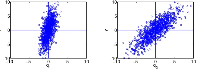
Q2∼N(0, σ22) represent hedged portfolios, wherec1 andc2 are the amounts invested in each portfolio. In this example, we takec1 = 2,c2 = 1, σ1 = 1 and σ2 = 3. The fact thatσ2 > σ1 implies that the second portfolio is more volatile than the first. The scatterplots of 1000 joint realizations ofq1, q2 andy in Figure 4 indicate thatQ2has more influence onY thanQ1. Hence, globally,Y is more sensitive toQ2thanQ1.
However, the local sensitivity si= ∂Q∂Yi fori= 1,2 yieldss1 = 2 ands2 = 1, indicating thatq1 is more sensitive. This reflects the amounts invested in the two portfolio rather than the effects of their volatility of the return. Hence the local sensitivity does not incorporate the nonlinear uncertainty structure over the global admissible parameter space nor the effect of parameter variability on the response.
In our HIV example, we are interested in how parameters affect the model response in the entire parameter space, rather than at some nominal parameter values. For this reason, we use global sensitivity analysis as a parameter selection technique and isolate influential parameters from noninfluential parameters. In the next section, we discuss three methods of parameter selection based on global sensitivity analysis and one method based on standard errors.
3
Parameter Selection Methods
The first of the four parameter selection methods that we discuss is termed the Partial Correlation, or Pear-son’s Correlations. This method quantifies the linear effect of parameters on the model response. Secondly, we detail the use of Sobol indices based on a variance-based, second-order Sobol decomposition. As an initial step, we examine and verify the accuracy of the second-order expansions. Thirdly, we consider the Morris screening method. We note that this method provides a mechanism of ranking parameters but does
−10 −5 0 5 10 −10
−5 0 5 10
q
1
y
−10 −5 0 5 10
−10 −5 0 5 10
q 2
y
not necessarily quantify their relative importance. Finally, we summarize the parameter subset selection detailed in [3]. This method quantifies the importance of parameters by comparing a dimensionless ratio of standard error and mean for each parameter.
3.1
Partial Correlation
We begin by computing partial correlations as detailed in [1]. For two random variables X and Y, the covariance is given by
cov(X, Y) =E[(x−E(X))(Y −E(Y))] =E(XY)−E(X)E(Y).
The partial correlation is then given by
ρXY =
cov(X, Y)
σXσY
. (4)
The partial correlation quantifies the degree to which two random variables are correlated. For example,
ρXY = 0 indicates thatX and Y are not correlated. We note that it does not imply that the two random variables are independent since (4) only quantifies linear dependencies between parameters. On the other hand,ρXY =±1 indicates a linear algebraic relation between the variables, in which case they are not jointly identifiable. Values greater than 0.5 generally indicate significant correlations. However, one must study the parameters with partial correlation values less than 0.5 for possible confounding factors or nonlinearities before determining insignificant.
For the HIV example, X = Qi denotes the random variable for the ith parameter, and Y is the ran-dom variable representing the model response. The partial correlation then quantifies the degree of linear correlation between a parameterqi and model responsey. We compute the correlation
ρqiy=
X
j
((qi)j−q¯i)(yj−y¯)
s X
j
((qi)j−q¯i)2X k
(yk−y¯)2
,
where ¯qi and ¯y are the means of qi and y, respectively. The number of function evaluations required to compute the partial correlation usingM Monte Carlo evaluations forpparameters is thenM ×p.
For this method, variables with large partial correlations are considered more influential on the response than those yielding small values ofρQiYi. For the portfolio model (3), this would reflect the results shown
in Figure 4, which indicate thatQ2is more influential than Q1.
3.1.1 Partial Correlation Results
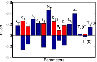
The partial correlation values are computed for the model (1) using M = 2000 function evaluations per parameter. The result is plotted in Figure 5 to provide visual comparison for the overall input-output correlation. Since we are interested in the magnitude of correlation values, the negative correlation values are also shown in the positive direction.
The result indicates thatNTis most correlated to the model response. Also,pT andk1are more correlated to the model response than other variables. On the other hand, two of the initial conditions,T1(0) andT1∗(0) are not correlated to the model response, implying that they have minimum influence.
3.2
Sobol Indices
−0.4 −0.2 0 0.2 0.4 0.6
Parameters
PCorr
pT
T1*(0)
T2(0)
ε
2
aT
d1
λ
T ε1
k1
NT
bE2
pEaA
T1(0)
aE
Figure 5: Partial correlation of the scalar response to the input parameters.
3.2.1 Sobol Decomposition
Sobol indices are based on a second-order High Dimensional Model Representation (HDMR) or Sobol rep-resentation
f(q)≈f0+ p
X
i=1
fi(qi) +
X
1≤i<j≤p
fij(qi, qj). (5)
Since the representation (5) is not unique, additional conditions are imposed to ensure the uniqueness of component functionsfi andfij. As detailed in [14, 16, 20, 21], each component function is uniquely specified by minimizing the functional
J =
Z
Γp "
f(q)− f0+ p
X
i
fi(qi) +· · ·+ X i1<···<is
fi1,···,isqi1,· · ·, qis) !#2
dq
subject to
Z
Γ
fi1,...,is(qi1, . . . , qis)dqik= 0
fork= 1, . . . , sands= 1, . . . , p.
The component functions are given by
fi =
Z
Γp−1
f(q)dq∼i (6)
fij =
Z
Γp−2
f(q)dq∼i,j (7)
where Γk= [0,1]k for a positive integerkand the notationdq∼i denotesdq1, . . . , dqi−1, dqi+1, . . . , dqp. The variance-based method employs the expansion (5) to quantify the contribution of each parameter to the variance of response. As detailed in [20], the total variance of response Y is given by
D= var(Y) =
Z
Γ
f2(q)dq−f02
wheref0is the mean response given by
f0=
Z
Γ
f(q)dq.
The total variance can be expressed as a sum of variances due to first-order and second-order parameter interactions by expressingD as
D= p
X
i=1
Di+
X
1≤i<j≤p
where
Di =
Z
Γ
fi2(qi)dqi
Dij =
Z
Γ2
fij2(qi, qj)dqi dqj.
The Sobol indices are then defined to be
Si=
Di
D, Sij = Dij
D , i, j,= 1, . . . , p.
Here Si are often called the importance measures or first-order sensitivity indices, and they measure the contribution of the parameterqi on the response variance. A large value ofSi implies stronger influence of parameterqi on the response variance. Similarly, Sij measures the contribution of parameter interactions between qi and qj on the response variance. Since the computation of first- and second- order sensitivity indices requiresp+p(p−1)2 model responses, we instead consider the total sensitivity indices
STi =Si+
p
X
j=1
Sij
which quantify the total effect of the parameterqi on the response [20].
3.2.2 Statistical Interpretation
The Sobol indices, along with the expansion terms and partial variances, have expectation or variance interpretations. Let
E(Y|qi) =
Z
Γp−1
f(q)dq∼i
E(Y|qi, qj) =
Z
Γp−2
f(q)dq∼{ij}
denote the expected response whenqi andqi, qj are fixed. The component functions are
f0=E(Y)
fi(qi) =E(Y|qi)−f0
fij(qi, qj) =E(Y|qi, qj)−fi(qi)−fj(qj)−f0. As detailed in [20],
Di= var[E(Y|qi)] and hence
Si=
var[E(Y|qi)] var(Y) .
Similarly, using the equality
Dij = var[E(Y|qi, qj)]−var[E(Y|qi)]−var[E(Y|qj)],
the total sensitivity index has the variance interpretation
ST i= 1−var[E(Y|q∼i)]
var(Y) =
E[var(Y|q∼i)]
var(Y) . (8)
The interpretation of E(Y|qi) and var[E(Y|qi)] is illustrated in Figure 6 from the portfolio example in
−10 −5 0 5 10 −10
−5 0 5 10
q
1
y
−10 −5 0 5 10
−10 −5 0 5 10
q 2
y
Figure 6: Response for fixed values of (a)q1 and (b)q2 illustratingE(Y|qi) and var[E(Y|qi)].
3.2.3 Sobol Indices Algorithm
Since the computation of the Sobol indices requires high-dimensional integration, the indices are approxi-mated numerically. If one usesM Monte Carlo evaluations to approximate the meanE(Y|qi) and repeats the
procedure M times to approximate the variance var[E(Y|qi)], a total of M2 evaluations will be required to
evaluate a single index. The total number of function evaluations required isM2p, which is computationally prohibitive for a large parameter dimensionsp. This motivated the author of [17] to provide a more efficient algorithm to compute Sobol indices that reduces the required evaluations to M(p+ 2), based on Sobol’s original approach in [21]. The algorithm was further improved by the authors of [18, 22] and is summarized here.
Algorithm
1. Create two sample matrices AandB
A=
q11 . . . q1i . . . qp1
..
. ...
qM
1 . . . qiM . . . qpM
, and B=
ˆ
q11 . . . qˆ1i . . . qˆp1 ..
. ...
ˆ
qM
1 . . . qˆiM . . . qˆpM
.
The entriesqji and ˆqij are quasi-random numbers drawn from the respective densities.
2. Create A(i)B
A(i)B =
q11 . . . qˆi1 . . . q1p
..
. ...
qM
1 . . . qˆMi . . . qMp
which is the matrixA except thatithcolumn is taken from B. Similarly, createBA(i).
3. Create Cwhich is the matrixB appended to matrixAsuch that
C=
A − B
The rows ofCare linearly independent, and this matrixC is used when estimating the total variance.
4. Compute column vectorsf(A),f(B),f(A(i)B) andf(BA(i)) by evaluating the model at input values from the rows of matrices A, B, A(i)B and B(i)A . Let f(A)j denote the output computed from the jth row of A. The computation off(A) and f(B) requires 2M model evaluations, whereas the evaluation of
5. Estimate the Sobol indices. The first-order Sobol indices are approximated by
Si= 1 M M X j=1 h
f(A)jf(B(i)A )j−f(A)jf(B)ji 1
2M
2M
X
j=1
f(C)jf(C)j− hf(C)i 2
(9)
and the total Sobol indices are approximated by
ST i= 1 2M M X j=1 h
f(A)j−f(A (i) B)j
i2 1 2M 2M X j=1
f(C)jf(C)j− hf(C)i2
. (10)
In the last step, variances are approximated using Monte Carlo approximation. The denominator in (9) and (10) is the approximation for the total variance with E(Y2) ≈ 1
2M
P2M
j=1f(C)jf(C)j and (E(Y))2 =
hf(C)i2. In (9), the term 1 M
PM
j=1f(A)jf(B (i)
A )j approximates E(E(Y|qi))2. In essence, we are taking the mean of responses when all input parameters are varied except qi. The effect of qi is fixed since the ith column is the same in bothAandBA(i).
The second term in (9),
1
M
M
X
j=1
f(A)jf(B)j,
represents the squared mean,f2
0, using the identify
f02=
Z
Γ2
f(x)f(x0)dxdx0.
This approximation is shown in [22] to reduce the loss of accuracy when computingD, compared to
f02≈
1 M M X j=1
f(A)j
1 M M X j=1
f(B)j
,
which is used in the previous versions of the algorithm.
The computation ofST i follows from the derivations in [12], which uses the approximation
E[var(Y|q∼i)]≈ 1
2M
M
X
j=1
h
f(A)j−f(A(i)B)ji 2
instead of the approximation
var[E(Y|q∼i)]≈ 1
M
M
X
j=1
f(A)jf(A(i)B)j−f02
in (8). The comparison of different versions of the algorithm can be found in [18].
3.2.4 Sobol Indices Results
0 0.05 0.1 0.15 0.2 0.25
Parameters
S T
i k1
aT NT
bE2
a
E
pEa
A
pT
T
2(0)
T1*(0) T1(0) d1
ε 1
ε 2
λ T
Figure 7: Sobol indicesST ifor 15 parameters.
3.2.5 Verification of the Sobol Decomposition
Since the accuracy of the Sobol indices depends on the accuracy of the approximated second-order Sobol representation, we test whether the function is accurately approximated by the second-order Sobol decom-position.
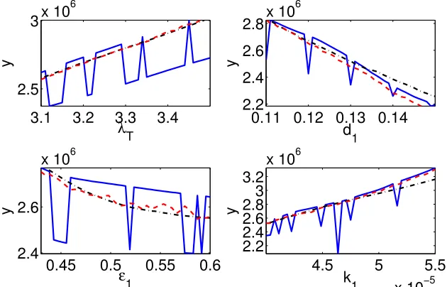
To ensure that we can adequately approximate the integrals, we consider four parametersq= [λT, d1, 1, k1] with values in the 4-D hypercube [3.1,3.5]×[0.11,0.15]×[0.43,0.60]×[4e-5, 5.5e-5]. We compute the model response usingn= 41 equally-spaced quadrature points in each dimension to evaluate the integrals (6) and (7). The function is expanded with a zero-th, first, second, third and fourth order component functions so that
f =f0+
X
i
fi(qi) +X i<j
fij(qi, qj) +
X
i<j<k
fijk(qi, qj, qk) +
X
i<j<k<h
fijkh(qi, qj, qk, qh).
In Figure 8, we plot the model response along with first- and second-order approximations, where the fixed parameter values are taken to beλT = 3.19, 1= 0.119, d1= 0.46825, k1= 4.3375e-5. The model response is represented by the blue solid line, while the first-order approximation and the second-order approximation are represented by dashed-dot black and by dashed red, respectively.
We note that both the first- and second-order approximations smooth out the jumps in the model
3.1
3.2
3.3
3.4
2.5
3
x 10
6
λ
Ty
0.11 0.12 0.13 0.14
2.2
2.4
2.6
2.8
x 10
6
d
1y
0.45
0.5
0.55
0.6
2.4
2.6
x 10
6ε
1y
4.5
5
5.5
x 10
−52.2
2.4
2.6
2.8
3
3.2
x 10
6k
1y
response, and they do not accurately represent the model response. There are little difference between the first-order and second-order approximations, which explains the similarity between the reported values of
Si and ST i. In the HIV model (1), the higher order interactions are non-negligible, and the second-order approximation is not sufficiently accurate to completely represent the model response. This may introduce some inaccuracy when determining the relative influence of parameters using the Sobol indices.
3.3
Morris Screening
The third method we consider is Morris screening [15, 17]. Screening methods rank the importance of parameters by averaging coarse difference relations termed elementary effects. The elementary effects are then used to compute sensitivity measures, based on the mean and variance, which represent the linear effect of parameters and the effect of interaction terms on the model response. Morris Screening employs neighbors to compute elementary effects, which reduces the total model evaluations by approximately a half. Whereas Morris Screening can only rank the parameter importance, and does not quantify the relative importance of each parameter, this method is significantly more efficient than computing Sobol indices. More details regarding the method can be found in [8, 20].
As with Sobol indices, we first map parameters to [0,1]. We also assume no prior information about parameters and hence take them to be uniformly distributed. This latter assumption can be modified if prior parameter information is available. The elementary effect is given by
di(q) =f(q1, . . . , qi−1, qi+ ∆, qi+1, . . . , qp)−f(q)
∆ =
f(q+ei)−f(q)
∆ ,
where ∆ is the step size chosen from the set ∆ ∈
1
`−1, . . . ,1− 1
`−1
. Constructed in this way, di
quantifies the approximate, large scale, local sensitivity at qi. We note that the step size is taken large to cover the entire parameter space. As detailed in [8, 15, 20], taking`to be even and choosing ∆ = 2(`−1)` has the advantage that it guarantees equal probability sampling from the distribution.
Let
dki = f(q
k+ ∆ei)−f(qk)
∆ (11)
be the elementary effect associated with theithparameter and kthsample. Forrsample points, the Morris indices for the parameterqi are
µ∗= 1
r
r
X
k=1
|dk s|
σ2= 1
r−1 r
X
k=1
(drs−µ)2, whereµ=1
r
r
X
k=1
dks.
The mean quantifies the individual effect of the input on output, whereas the variance incorporates the influence of parameter interactions. Since we must consider both the mean and the variance, we rank the parameter using the quantitypµ∗2+σ2 when ordering the importance of parameters. Computing (11) requires two model evaluations per parameter per sample. Hence, a total of 2prmodel evaluations is required to compute the Morris indices,µ∗andσ2. As detailed in Algorithm 3.3.1 below, taken from [8], one employs neighbors to reduce the number of total model evaluations to (p+ 1)r.
3.3.1 Morris Screening Algorithm
1. Create a (p+ 1)×pmatrixAwith ones in the lower triangle such that
A=
0 0 . . . 0 1 0 . . . 0 ..
. . .. 1 1 . . . 1
2. Choose the step size ∆. Unless specified by the user, take ∆ = ` 2(`−1). 3. Select a starting vector q∗.
4. Construct a diagonal matrixD∗, whose entries are randomly chosen from{−1,1}. 5. Calculate the sampling matrixAsas the following
As=Jp+1,pq∗+ ∆
2 [(2A−Jp+1,p)D ∗+J
p+1,p]P∗,
where Ji,j is ai×j matrix with all ones andP∗ is a p×ppermutation of the identity matrix. 6. If the parameters are not defined in the hypercube [0,1]pand insteadq∈[`b
i, ubi] fori= 1, . . . , p, take
`b= [`b1, `b2, . . . ..., `bp] andub= [ub1, ub2, . . . , ubp]. The sampling matrix is then scaled to match the range of parameters
C=Jp+1,1`b+As(D(ub−`b)) (12) where D(ub−`b) is a diagonal matrix with entriesub−`b.
7. Compute the elementary effect for s= 1, . . . , p. We letCk denote thekthrow ofC. Then
ds=
f(Ci)−f(Cj)
∆ , (13)
where iandj denote the indices such thatithrow andjthrow differ in thesthentry.
8. Repeat the steps 1−7 forrsamples. The Morris meanµ∗andσ2are computed by taking the average of the local elementary effect
µ∗=1
r
r
X
k=1
|dk s|
σ2= 1
r−1 r
X
k=1
(drs−µ)2, whereµ= 1
r
r
X
k=1
dks.
We note that the denominator of (13) in Step 7 is ∆ for allqi, i= 1, . . . , p. The elementary effects must be computed using the scaled step size, even though model responses are computed at the parameter values, which are mapped using (12).
3.3.2 Morris Indices Results
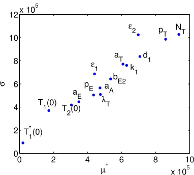
We use`= 20,r= 50 and the default step size ∆ =`/2(`−1). We plot the elementary effectsµ∗andσ2 in Figure 9 to visualize those parameters that are more influential. The most influential parameter is againNT followed bypT and2. The results also coincide with those from Partial Correlation and Sobol for the least influential parameters, which areT1∗(0) andT1(0). The parameteraE, which is one of the least influential parameters in Partial Correlation and Sobol afterT1∗(0) andT1(0), is still ranked low. One difference with Morris screening, however, is that all three initial conditions are identified as minimally influential.
3.4
Parameter Subset Selection
0 2 4 6 8 10 x 105 0 2 4 6 8 10 12x 10
5
µ*
σ
ε2 p
T
k1
pE
T1*(0)
T2(0) aE
ε1
λT aA
bE2 aT d1
NT
T1(0)
Figure 9: Morris µ∗ andσcomputed using the Morris screening algorithm.
For a vector of parametersq= [q1, . . . , qp], we first require the optimal parameter estimates ofq, denoted by ˆq= [ˆq1, . . . ,qˆp], and the corresponding standard errors,SE= [SE1, . . . , SEp]. Then, given the parameter vectorqof sizepand a numbernp≤p, the subset selection algorithm returns a set of parameters of sizenp that minimizes the selection score,
α(ˆq) =|ν(ˆq)|.
Here,ν(ˆq) = [ν(ˆq1), . . . , ν(ˆqnp)]
T, andν(ˆqi) is the coefficient of variation for ˆq
i defined by
ν(ˆqi) =SEi ˆ
qi
, i= 1, . . . , np.
The set of parameters with the smallest selection score givesnp most influential parameters.
3.4.1 Optimal Parameter Estimates
This technique utilizes time-dependent responses. Following the strategy in [3], we employ the responses
z1=T1+T1∗+T2+T2∗
z2=VI+VN I,
(14)
which are the total CD4+ T-cells and the total RNA copies, respectively. We assume a statistical model of the form
Y1i=z1(t i
1;q0) +e i
1, i= 1,2, , . . . , N1
Y2j=z2(tj2;q0) +zγ2ej2, j= 1,2, . . . , N2,
(15)
where yi1 and y j
2 are realizations of the random variables Y i 1 and Y
j
2, respectively, and e i 1 and e
j
2 are in-dependently identically distributed such that E[ei
1] = E[e j
2] = 0 with Var(ei1) = σ12 and Var(e j
2) =σ22 for
i= 1, . . . , N1, j= 1, . . . , N2. Also,q0 represents the hypothesized true parameter values. The weighted least squares estimator is given by
ˆ
q= arg min q∈Q 1 N1 N1 X i=1 (yi
1−z1(ti1;q0))2
σ2 1 + 1 N2 N2 X j=1
(y2j−z2(t j 2;q0))2
σ2 2z
2γ 2 (t
j 2;q0)
(16)
where the variance components are given by
σ12(q0) = 1
N1−dim(q0) N1
X
i=1
(y1i−z1(ti1;q0))2
σ22(q0) =
1
N2−dim(q0) N2
X
j=1
(y2j−z2(tj2;q0))2
z2γ2 (tj2;q0) .
The value of γ is determined based on the underlying assumption for the statistical models (15). More specifically, it was determined in [3, 7] that choosingγ= 1.2 results in the residuals being approximately iid, which is an assumption for the model (15). For this reason, the parameter estimation was performed with
γ= 1.2.
Since the estimates in (16) and (17) involve an unknown, to-be-estimated parameter vectorq0, the optimal parameter is estimated iteratively with the initial varianceσ2
k = 1 fork= 1,2 and the weightsz 2γ 2 (t
j
2;q0) = 1 forj= 1, . . . , N2. We summarize the parameter estimation algorithm from [3].
Parameter Estimation Procedure Algorithm
1. Obtain initial estimate ˆq(0) using (16) with σ2
k = 1 for k = 1,2 and the weights z 2γ 2 (t
j
2;q0) = 1 for
j = 1, . . . , N2.
2. Compute the variancesσ2
k using (17), and the weightsz 2γ 2 (t
j
2;q0) withq0replaced by ˆq(0).
3. Initialize the iteration counter`with the value 1.
4. Do each of the following:
• Compute ˆq(`)using (16) with current variancesσ2
k and weights z 2γ 2 (t
j
2; ˆq(`−1)).
• Update the variancesσ2
k using (17) and the weightsz 2γ 2 (t
j
2; ˆq(`−1)) withq0, ˆq(`−1)replaced by ˆq(`).
• Compute ∆ε=||[ˆq(`)−qˆ(`−1)]./[ˆq(`−1)]||.
• Increment`by 1.
5. If ∆ε> ε, go back to Step 4. Otherwise, terminate the algorithm.
In this algorithm, ε is a user-defined threshold tolerance for a termination criterion, and ./ denotes element-by-element division.
3.4.2 Computing Standard Errors
The parameter subset selection algorithm also requires the computation of standard errors for the parameters. The standard errors are computed using standard asymptotic theory for generalized least squares (GLS) estimators qn
GLS following the procedure discussed in [3]. The p×p Fisher Information Matrix (FIM) corresponding toz1 andz2 in (14) is approximated by
ΣN1+N2
0 ≈ N1 X i=1 1 σ2 1(ˆqn)
∂z1(ti 1; ˆqn)
∂qk
∂z1(ti 1; ˆqn)
∂q` + N2 X j=1 1 σ2 2(ˆqn)z
2γ 2 (t
j 2; ˆqn)
∂z2(tj2; ˆqn)
∂qk
∂z2(tj2; ˆqn)
∂q` k,` (18)
whereσ21 andσ22 are defined in (17) withq0 approximated by ˆqn.
To approximateq0, we first letz1=T1+T1∗+T2+T2∗andz2=VI+VN I. The sensitivities are computed by solving the system of equations
d dt ∂z m ∂q
=∂gm
∂x
∂x
∂q
+dgm
dq , m= 1,2.
Here, xandq respectively denote the state variables and the parameters being estimated. Define the 2×p
matrices
Di1(q0) =
∂z1 ∂q1(t
i
1;q0) . . . ∂z∂q1p(t
i 1;q0) 0 . . . 0
fori= 1, . . . , N1
Di2(q0) =
0 . . . 0
∂z1 ∂q1(t
i
1;q0) . . . ∂z∂q1p(t
i 1;q0)
fori= 1, . . . , N2.
and define the 2×2 matrix
V0(t;q0) =
σ2
1 0
0 σ2 2z
2γ 2 (t;q0)
The matricesDi 1 T
V0−1(ti
1)Di1andD j 2 T
V0−1(tj2)D2j respectively have entries
Fk,`1,i(q0) =σ−21 ∂z1 ∂qk
(ti1;q0)∂z1
∂q`
(ti1;q0), k, `= 1, . . . , p, i= 1, . . . , N1
Fk,`2,j(q0) =σ−22 z −2γ 2 (t
j 2;q0)
∂z2
∂qk (tj2;q0)
∂z2
∂q`
(tj2;q0), k, `= 1, . . . , p, i= 1, . . . , N2
Then, we define thep×pFisher matrixF(q0) =Fk,`(q0) with entries
Fk,`(q0) = N1
X
i=1
Fk,`1,i(q0) + N2
X
j=1
Fk,`2,j(q0). (19)
The approximate Fisher matrix (18) is obtained by evaluating (19) at ˆqn ≈q
0. Using the Fisher matrix approximations,F, the standard errors for ˆqn
k, k= 1, . . . , p, are given by
SEk=SE(ˆqkn) =
q
(F−1(ˆqn))k,k.
It is illustrated in [20] that the standard errors are related to the variance of parameter estimates so they quantify the uncertainty of each parameter. Parameters with small standard errors are estimated with a high degree of certainty, so one can conclude that their impact on the response is influential. On the other hand, parameters that are noninfluential have minimal impact on responses, which yields more uncertainty and larger standard error when estimating optimal parameter values.
3.4.3 Parameter Subset Selection Results
As presented in [3], we compile the parameters that give the smallest selection score for a given number of parameters in the set,np, in Table 4. We note that these results are patient-dependent andNT was not in the top three for the considered patient. For other patients,NT is in the top 3.
For example, if we want a subset of three parameters that are most influential, we select λT, 2 andpT. In this way, the parameter subset selection algorithm selects a set of parameters for a given number ofnp; however, it does not specify which parameter is more influential among the selected parameters. We see that the set fornp=kis a subset fornp=k+ 1 for allk, exceptk= 2. Unlike Partial Correlation, Sobol indices and Morris indices, Parameter Subset Selection has a local sensitivity approach since the sensitivity matrices are computed around the mean values. Nevertheless, we can use the parameter subset selection result to provide a comparison regarding which parameters to include when we specify a number of parameters to choose from the entire set.
4
Comparison and Verification of Parameter Selection Techniques
In this section, we illustrate two techniques for verifying the accuracy of the parameter selection techniques. We first verify the results provided by the global sensitivity techniques, which rank the impact or influence of the inputs, and the parameter subset selection. We do this in Section 4.1 by comparing the input rankings provided by the four methods. In Section 4.2, we verify the noninfluential inputs by comparing responses obtained with various input combinations.
4.1
Verification of Input Rankings
np NT λT 2 pT pE T2(0) T1(0) 1 d1 bE2 aE aT k1 aA T1∗(0)
1 x
2 x x
3 x x x
4 x x x x
5 x x x x x
6 x x x x x x
7 x x x x x x x
8 x x x x x x x x
9 x x x x x x x x x
10 x x x x x x x x x x
11 x x x x x x x x x x x
12 x x x x x x x x x x x x
13 x x x x x x x x x x x x x
14 x x x x x x x x x x x x x x
15 x x x x x x x x x x x x x x x
Table 4: Parameter subset selection results from [3].
To provide a comparison among the four methods, we summarize in Table 7 and 8 the parameters to be selected for a given number of parameters. In Table 7 and 8, PCorr, S, M and PSS respectively denote Partial Correlation, Sobol indices via Saltelli algorithm, Morris indices and Parameter Subset Selection. For Partial Correlation, Sobol indices and Morris indices, np influential parameters correspond to the top np parameters from Table 6.
Overall, Partial Correlation is the cheapest method to measure linearity between parameters and response. This often corresponds to the first order Sobol indices. Computing Sobol indices is expensive and it becomes prohibitively slow as the number of input parameters increases. For a model with a moderate number of input parameters, we can apply Morris screening. This employs neighbors to compute statistically averaged local, very coarse approximations to derivatives. Morris indices are a good measure to isolate influential parameters from noninfluential parameters with much fewer evaluations than Sobol indices. Finally, the parameter subset selection algorithm provides sensitivity in terms of uncertainties involved in the estimation process. The noninfluential parameters determined by this method did not match the results from the other three.
In terms of accuracy, Sobol indices measure the first- and second-order interaction effects of parameters most accurately. However, we showed that second-order Sobol decomposition may not be sufficiently accurate depending on the model. Even though the Sobol indices are widely used for global sensitivity analysis, one must always consider the accuracy of Sobol decomposition as an approximation to the model before applying the results of Sobol indices.
When the parameter selection techniques are applied to the HIV model, we found that certain parameters are determined highly influential by all four methods. An example of highly influential parameters are NT andpT. These parameters respectively represent the number of RNA copies during the process of T1∗ lysis and net proliferation ofT1 and T1 due to clonal expansion and programmed contraction. We also observed that both1and2were ranked above average in their importance. This is essential in designing the optimal control for drug therapy. We see from our global sensitivity analysis that the relative effectiveness of protease inhibitor,2, has more affect on the model response than that of reverse transcriptase inhibitor, 1. On the other hand, for our specific response, it was shown that initial conditionsT1(0), T1∗(0) andT2(0) do not play a strong role in determining the response.
4.2
Verification of Noninfluential Inputs
Method Sensitivity Measure Description Cost Partial
Correlation
Degree of linear corre-lation between param-eters and response
Ranks the parameters in the order of strong linear correlation to response. Considers linearity only.
M model evaluations for M Monte Carlo samples.
Sobol by Saltelli
First order Sobol Si and total sensitivity in-dicesST i
A type of variance-based method. Uses 2nd order Sobol decomposition. Ranks the parameters and quantifies relative importance. Measures the effects of in-dividual parameters as well as interac-tion terms.
2M(p+ 1) model eval-uations for M Monte Carlo samples and p
parameters.
Morris Screening
Mean µ∗i and variance
σ2 of elementary ef-fects
Averages coarse local derivative ap-proximations. Only ranks parameters. Employs neighbors to reduce the cost.
(p + 1)r model eval-uations for r sample points for averaging andpparameters. Parameter
Subset Selection
np parameters with minimum uncertainty
Provides identifiable subset of np pa-rameters. Requires the optimal param-eter estimate ˆqand standard errorsSE.
C(p, np) subsets to check for minimum uncertainty for sub-set of np parameters amongpparameters.
Table 5: Summary of parameter selection techniques.
Partial Correlation Sobol by Saltelli Morris Indices Rank Parameter Corr(q, y) Parameter Si ST i Parameter
p
µ∗2+σ2
1 NT 4.608e-1 NT 1.455e-1 2.134e-1 NT 1.390e+6
2 pT 3.964e-1 pT 1.046e-1 2.038e-1 pT 1.308e+6
3 k1 2.970e-1 k1 1.066e-1 1.335e-1 2 1.240e+6
4 d1 -2.630e-1 2 7.879e-3 1.329e-1 d1 1.096e+6
5 bE2 -2.526e-1 d1 6.276e-2 1.141e-1 k1 9.876e+5
6 aT 2.178e-1 aT 5.568e-2 9.541e-2 aT 9.824e+5
7 2 -2.167e-1 1 5.426e-2 7.849e-2 bE2 8.371e+5
8 aA 2.111e-1 bE2 8.948e-2 7.723e-2 1 8.161e+5
9 pE -1.789e-1 aA 3.727e-2 5.458e-2 aA 7.378e+5
10 λT 1.774e-1 pE 2.013e-2 5.384e-2 λT 6.971e+5
11 1 -1.601e-1 λT 4.682e-2 4.626e-2 pE 6.666e+5
12 T2(0) 1.487e-1 T2(0) -1.032e-2 4.266e-2 aE 5.662e+5
13 aE -9.089e-2 aE 1.057e-2 1.943e-2 T2(0) 5.180e+5
14 T∗
1 2 3 4
PCorr S M PSS PCorr S M PSS PCorr S M PSS PCorr S M PSS
λT x x x
d1 x x
1
k1 x x x x
aT
2 x x x x x
NT x x x x x x x x x x x x x x x
bE2
aE
pE
aA
pT x x x x x x x x x x x
T1(0)
T1∗(0)
T2(0)
5 6 7 8
PCorr S M PSS PCorr S M PSS PCorr S M PSS PCorr S M PSS
λT x x x x
d1 x x x x x x x x x x x x
1 x x x x
k1 x x x x x x x x x x x x
aT x x x x x x x x x
2 x x x x x x x x x x x x x x
NT x x x x x x x x x x x x x x x x
bE2 x x x x x x x
aE
pE x x x x
aA x
pT x x x x x x x x x x x x x x x x
T1(0) x x
T1∗(0)
T2(0) x x x
9 10 11 12
PCorr S M PSS PCorr S M PSS PCorr S M PSS PCorr S M PSS
λT x x x x x x x x x x x x
d1 x x x x x x x x x x x x x x x x
1 x x x x x x x x x x x x x x
k1 x x x x x x x x x x x x
aT x x x x x x x x x x x x x
2 x x x x x x x x x x x x x x x x
NT x x x x x x x x x x x x x x x x
bE2 x x x x x x x x x x x x x x x
aE x x x
pE x x x x x x x x x x x x x
aA x x x x x x x x x x x x
pT x x x x x x x x x x x x x x x x
T1(0) x x x x
T1∗(0)
T2(0) x x x x x x
13 14
PCorr S M PSS PCorr S M PSS
λT x x x x x x x x
d1 x x x x x x x x
1 x x x x x x x x
k1 x x x x x x x x
aT x x x x x x x x
2 x x x x x x x x
NT x x x x x x x x
bE2 x x x x x x x x
aE x x x x x x x x
pE x x x x x x x x
aA x x x x x x x
pT x x x x x x x x
T1(0) x x x x
T1∗(0) x
T2(0) x x x x x x x x
Verification Procedure
1. For a set of np influential parameters, samplen= 1000 parameter values from their respective distri-butions. For the results reported here, we took the distributions to be uniform with lower and upper bounds summarized in Table 3.
2. Fixp−np noninfluential parameters at pre-specified values, which we take to be the lower bounds of the parameters.
3. Compute the model response with parameter values from Steps 1 and 2.
4. Construct probability density function using a kernel density estimation.
We then compare the densities for the model responses where all parameters are sampled randomly. We construct densities for np = 8,10,12,14 influential parameters. That is, we examine four cases where the numbers of fixed parameters are 7, 5, 3 and 1, and plot the densities along with the density obtained by varying all the parameters. In Figure 10 (a) and (b), we see that we have fixed too many parameters. In Figure 10 (c), densities using Partial Correlation, Sobol and Morris match the sample density, whereas the density from parameter subset selection does not match the rest. This is reasonable since the influential parameters determined via Partial Correlation, Sobol and Morris indices are very similar as shown in Table 7. Finally in Figure 10 (d), we see that all four methods give comparable densities. The agreement of densities indicates that the parameter T∗(0) was determined to be noninfluential and it did not affect the output significantly. Moreover, this is the only parameter that can be fixed without affecting this output.
1 2 3 4 5
x 106 0
0.5 1 1.5x 10
−6
Model Response
1 2 3 4 5
x 106 0
0.5 1 1.5
2x 10
−6
Model Response
Random PCorr Sobol Morris PSS
(a) (b)
1 2 3 4 5
x 106 0
0.5 1 1.5x 10
−6
Model Response
1 2 3 4 5
x 106
0 0.2 0.4 0.6 0.8
1x 10
−6
Model Response
(c) (d)
Figure 10: Densities obtained by fixing (a) 7, (b) 5, (c) 3 and (d) 1 least influential parameters. The density in solid is obtained by varying all the parameters.
Parameter Partial Correlation S ST µ∗ σ2
q1 0.690 0.498 0.516 1 0.980
q2 -0.700 0.481 0.498 1 1.020
Table 9: Sensitivity measures fory=q1−q2.
learned that fixing one parameter resulted in insignificant variability of sample densities. This verification requires additional model evaluations and there is not a simple way to check which parameters are influential just by observing sensitivity measures.
Second, even if we are successful at isolating influential parameters, the parameter identifiability issues may still remain. Consider a simple example
y=q1−q2
with q1, q2 ∼ U(0,1). As we can see from the sensitivity measures summarized in Table 9, q1 and q2 are equally influential. Suppose that we have the observationy= 0. It is easy to see that parameter estimation using this observation will fail to estimate the densities of q1 andq2 correctly since there are several values ofq1 andq2that match the observation. Therefore, unless some prior knowledge is specified, q1 and q2 are unidentifiable.
This simple example illustrates that determining influential parameters may not eliminate parameter identifiability issues completely. In this regard, the parameter subset selection algorithm has the advantage that the selected subset is identifiable. Since Partial Correlation, Sobol and Morris methods only determine influential parameters, care must be exercised if these parameter selection techniques are used to isolate identifiable parameters for model calibration.
5
Conclusion
In this paper, we examined parameter selection techniques based on global sensitivity analysis and compared the results to a local sensitivity-based method originally performed on the model (1). Four parameter selection techniques were applied to the HIV model (1) to determine the set of influential parameters. This process enables us to fix the noninfluential parameters and hence reduce the parameter dimensions for subsequent uncertainty quantification. We also showed that the accuracy of Sobol indices depends greatly on the model. In our HIV model, the second-order decomposition was not sufficiently accurate to represent the response. If one is interested in determining parameter identifiability issues, then it is recommended that one uses the parameter subset selection algorithm since it returns a set of identifiable parameters with smallest uncertainty.
Acknowledgement
The research of RCS and HTB was respectively supported in part by the Air Force Office of Scientific Research (AFOSR) through the grants AFOSR FA9550-11-1-0152 and AFOSR FA9550-12-1-0188.
References
[1] B. M. Adams, M. S. Ebeida, M. S. Eldred, J. D. Jakeman, L. P. Swiler, W. J. Bohnhoff, K. R. Dalbey, J. P. Eddy, K. T. Hu, D. M. Vigil, L. E. Bauman, and P. D. Hough. Dakota, a multilevel parallel object-oriented framework for design optimization, parameter estimation, uncertainty quantification, and sensitivity analysis: Version 5.3.1 user’s manual. Sandia National Labs Report, No. SAND2010-2183, 2013.
[2] Y. Bang, H. S. Abdel-Khalik, and J. M. Hite. Hybrid reduced order modeling applied to nonlinear models. Internat. J. Numer. Methods Engrg., 91(9):929–949, 2012.
[3] H. T. Banks, R. Baraldi, K. Cross, K. Flores, C. McChesney, L. Poag, and E. Thorpe. Uncertainty Quan-tification in Modeling HIV Viral Mechanics. Technical report, CRSC-TR13-16, NC State University, Raleigh, NC, 2013. Journal of Theoretical Biology, submitted.
[4] H. T. Banks, A. Cintr´on-Arias, and F. Kappel. Parameter selection methods in inverse problem formu-lation. InMathematical modeling and validation in physiology, volume 2064 ofLecture Notes in Math., pages 43–73. Springer, Heidelberg, 2013.
[5] H. T. Banks, M. Davidian, S. Hu, G. M. Kepler, and E. S. Rosenberg. Modelling HIV immune response and validation with clinical data. J. Biol. Dyn., 2(4):357–385, 2008.
[6] H. T. Banks, S. L. Ernstberger, and S. L. Grove. Standard errors and confidence intervals in inverse problems: sensitivity and associated pitfalls. J. Inverse Ill-Posed Probl., 15(1):1–18, 2007.
[7] H. T. Banks and H. T. Tran. Mathematical and experimental modeling of physical and biological pro-cesses. Textbooks in Mathematics. CRC Press, Boca Raton, FL, 2009.
[8] F. Campolongo and A. Saltelli. Sensitivity analysis of an environmental model: an application of different analysis methods. Reliability Engineering & System Safety, 57(1):49–69, 1997. The Role of Sensitivity Analysis in the Corroboration of Models and its Links to Model Structural and Parametric Uncertainty.
[9] A. Cintr´on-Arias, H. T. Banks, A. Capaldi, and A. L. Lloyd. A sensitivity matrix based methodology for inverse problem formulation. J. Inverse Ill-Posed Probl., 17(6):545–564, 2009.
[10] R. Confalonieri, G. Bellocchi, S. Bregaglio, M. Donatelli, and M. Acutis. Comparison of sensitivity analysis techniques: A case study with the rice model WARM. Ecological Modelling, 221(16):1897– 1906, 2010.
[11] P. G. Constantine, E. Dow, and Q. Wang. Active subspace methods in theory and practice: applications to kriging surfaces. SIAM J. Sci. Comput., 36(4):A1500–A1524, 2014.
[12] M. J. W. Jansen. Analysis of variance designs for model output. Computer Physics Communications, 117(1–2):35–43, 1999.
[13] G. Lillacci and M. Khammash. Parameter estimation and model selection in computational biology.
PLoS Comput. Biol., 6(3):e1000696, 17, 2010.
[14] X. Ma and N. Zabaras. An adaptive high-dimensional stochastic model representation technique for the solution of stochastic partial differential equations. J. Comput. Phys., 229(10):3884–3915, 2010.
[16] H. Rabitz and ¨O. F. Alı¸s. General foundations of high-dimensional model representations. J. Math. Chem., 25(2-3):197–233, 1999.
[17] A. Saltelli. Making best use of model evaluations to compute sensitivity indices. Computer Physics Communications, 145(2):280–297, 2002.
[18] A. Saltelli, P. Annoni, I. Azzini, F. Campolongo, M. Ratto, and S. Tarantola. Variance based sensitivity analysis of model output. Design and estimator for the total sensitivity index. Comput. Phys. Comm., 181(2):259–270, 2010.
[19] A. Saltelli, M. Ratto, T. Andres, F. Campolongo, J. Cariboni, D. Gatelli, M. Saisana, and S. Tarantola.
Global sensitivity analysis. The primer. John Wiley & Sons, Ltd., Chichester, 2008.
[20] R. C. Smith. Uncertainty Quantification: Theory, Implementation and Applications. Society for Indus-trial and Applied Mathematics (SIAM), Philadelphia, PA, 2014.
[21] I. M. Sobol’. Global sensitivity indices for nonlinear mathematical models and their Monte Carlo estimates. Math. Comput. Simulation, 55(1-3):271–280, 2001. The Second IMACS Seminar on Monte Carlo Methods (Varna, 1999).
[22] I. M. Sobol’, S. Tarantola, D. Gatelli, S. S. Kucherenko, and W. Mauntz. Estimating the approximation error when fixing unessential factors in global sensitivity analysis. Reliability Engineering & System Safety, 92(7):957–960, 2007.

![Table 2: Nominal values of parameters and initial conditions from [3].](https://thumb-us.123doks.com/thumbv2/123dok_us/1629043.1202962/5.612.149.461.599.676/table-nominal-values-parameters-initial-conditions.webp)
![Figure 6: Response for fixed values of (a) q1 and (b) q2 illustrating E(Y |qi) and var[E(Y |qi)].](https://thumb-us.123doks.com/thumbv2/123dok_us/1629043.1202962/10.612.139.465.64.179/figure-response-for-xed-values-and-illustrating-and.webp)
![Table 4: Parameter subset selection results from [3].](https://thumb-us.123doks.com/thumbv2/123dok_us/1629043.1202962/18.612.100.511.57.255/table-parameter-subset-selection-results-from.webp)
