Frequency estimation and tracking by two layered iterative DFT with re sampling in non steady states of power system

R E S E A R C H

Open Access

Frequency estimation and tracking by

two-layered iterative DFT with re-sampling in

non-steady states of power system

Hui Li

Abstract

Frequency deviation off the nominal one is incurred by sudden changes of frequency and could introduce harmonics and inter-harmonics in the power system, which influences the accuracy of frequency estimation with method of discrete Fourier transform (DFT). A two-layered iterative DFT (TLI-DFT) with re-sampling was presented to measure the frequency in non-steady states. A simple frequency estimation method named exponential sampling is amended to calculate the initial sampling frequency in the inner-layered process of the DFT iteration. In reality, frequencies of two consecutive cycles are always interrelated with each other, so an idea of frequency tracking by outer-layered DFT between cycles is adopted. TLI-DFT can track the frequency in non-steady state in different scenarios, e.g., sudden and random frequency change, signal modulated by a cosine signal, and contaminated by decaying direct current offsets. Mean squared error of measured frequency, rate of change of frequency, and total vector error at different transient conditions indicate that the proposed algorithm is valid and more accurate than the traditional one in the non-steady states of a power system.

Keywords: Synchrophasor, Frequency measurement, Frequency tracking, Transient condition, Discrete Fourier transform (DFT), Re-sampling

1 Introduction

Protecting and controlling of the smart grid require accurate and timely estimation of frequency. Measurement of frequency provides information of state estimation in the power networks around the wide area measurement sys-tem. The signal in a power system is easy to be distorted by harmonics, inter-harmonics, decaying direct current (DC) offset, and to be modulated in dynamic states. Therefore, methods of frequency estimation and measurement should have the ability of frequency-tracking under noisy, distorted, and distributed circumstances.

In the past few decades, many researchers have put emphasis on frequency measurement and analysis, and kinds of frequency estimation strategies have been reported, e. g., zero crossing [1, 2], least error squares [3], Newton

approach [4], Kalman filter [5–7], prony algorithm [8], arti-ficial neural networks [9], discrete Fourier transform (DFT), fast Fourier transform (FFT) [1, 10,11] and demodulation technique [1]. DFT algorithm is the most well-known method for its capabilities of harmonics rejection and im-plementation of recursion. It is preferable for its availability, understandability, and simplicity when it is implemented by advanced digital signal processing chips.

Full-cycle DFT is a kind of window-based method requiring integral samples in each cycle. If the number of samples in a window is not an integer, which is com-mon because of some off-nominal components in reality, DFT may provide certain errors [12]. DFT can approxi-mate the instantaneous frequency, suppress the har-monics and smooth the noise by least squares method [13] in a steady state. However, the fundamental fre-quency of a signal would change and this signal may contain many off-nominal components as listed above, in which the decaying DC offset cannot be eliminated by simple DFT.

Correspondence:[email protected]

1_{College of Information Science and Technology, Hainan University, Haikou,}

China

2_{Engineering Research Center of Marine Communication and Networks,}

Hainan Province, Haikou, China

The fixed sampling rates are adopted by most data acquisition systems including the power system. It con-tains some drawbacks in frequency estimation and measurement. As a uniform sampling method, the sam-pling period of traditional DFT is constant. A simple frequency estimation method via exponential sampling and dyadic rational was provided in [14]. Other kinds of non-uniform sampling methods, e.g., log-time sam-pling [15], extended staggered under-sampling [16], logarithmic sampling [17], and near optimal sampling [18] were introduced. These sampling methods indicate that designing of phase-locked loop is important [19, 20]. Methods such as higher-order lags of the sample auto-correlation [21] and high-order Yule-Walker esti-mation [22] were utilized in calculating the sinusoidal frequency, and a variable-window-based algorithm for frequency tracking and phasor estimation was narrated in [23].

In this paper, a new method for frequency estima-tion and tracking was proposed, in which DFT algo-rithm iterates with re-sampling to confront frequency change in dynamic states of a power system. In each cycle, precise frequency estimation is accomplished by iterative DFT. In the following cycle, the initial sam-pling frequency is given by this converged frequency, and so on. The proposed iterative DFT by re-sampling is a two-rounded process to provide precise frequency estimation and frequency tracking ability dynamically in a power system.

The algorithm of frequency estimation by DFT was presented and the error caused by an off-nominal sig-nal was asig-nalyzed in Section 2. Frequency tracking by iterative DFT with re-sampling was discussed. Recom-mended by IEEE Std. C37.118 [24, 25], analysis of three types of step-changed signal was made in Sec-tion 3. Performance of the new algorithm in different scenarios was shown in Section 4. Additional discus-sions about wavelet transform were made in Section5. Conclusions were given in Section 6. Some formula derivations and auxiliary figures were provided in the Appendix.

2 Method of frequency estimation by DFT

2.1 Algorithm of classic DFT

DFT can provide the amplitude and phase angle of phasor and the frequency by way of differentiating the phase angles. Suppose the nominal voltage or current signal in a nominal power system is

x tð Þ ¼Acosðωtþφ₀Þ ð−∞<t<∞Þ; ð1Þ

where ω and A are the angular frequency and ampli-tude respectively. ω is supposed to be 2πf0, f0 is the

nominal frequency, and φ0 is the initial phase angle.

In order to precede the DFT calculation, signal is always truncated and finite samples should be taken by kinds of windows. The process of making a phasor estimation will require sampling the waveform over some interval of time which can lead to some confu-sion if the number of samples is not an integer in a window. The magnitude is compensated by dividing the magnitude with a sine at the actual signals fre-quency. The 2-cycle triangular window produces a faster roll off than a standard 1s-cycle rectangular window, but the frequency deviation is spread with an additional factor of 1.625 to increase compensation [25]. A simple rectangular window is adopted in this study. By the way, the length of a rectangular window could be selected easily and arbitrarily according to the requirements of accuracy and computational bur-den. DFT converts the equally spaced and uniform samples into a finite combination of complex sinu-soids, ordered by their frequency. According to DFT, a phasor is calculated by

Xk¼ within the length of a rectangular window;kis the order of harmonic; especially if k= 1, it stands for the phasor of the nominal component. The amplitudes and phase angles ofkth harmonics are

Xk

where atan stands for the arctan function. X_{k_}real and Xk_imagare real part and imaginary part ofXk. According to Eq. 2 and Eq. 3, if k= 1, the phasor of the nominal

where X1_real is the real part of the phasor of nominal

component, andX1_imagis the imaginary part. In front of

X1¼Aejφ0: ð5Þ

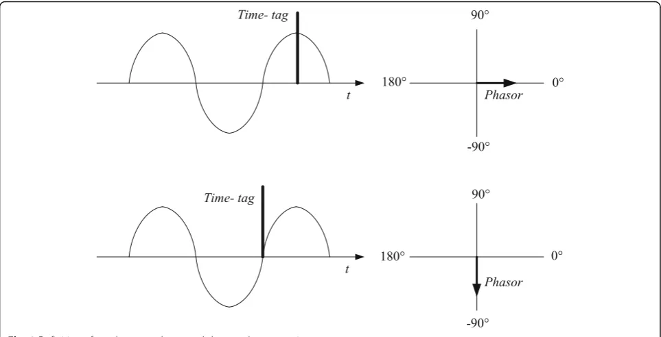
Definition of synchronous phasor is shown in Fig.1, in which the peak of the sine/cosine signal coincides with the time-tag, so the angular is 0°; if the signal crosses zero at the time-tag, it produces −90° according to the IEEE Std. C37.118 [24–26].

2.2 Frequency estimation by classic DFT

The synchronous phasor (synchrophasor) is defined as a complex number, representing the fundamental fre-quency component of a voltage or current, with an ac-companying time-tag defining the time instant for which the phasor measurement is performed [27]. Serial syn-chrophasors are calculated by shifting windows at each sampling time t_r=rT_s, r= 0,1,2,…,+∞, where T_s is the sampling interval,T_s= 1/f_s. A synchrophasor at timet_ris represented as

Xr 1¼

2

N

X

N−1

n¼0

x nð Þe−j2π

Nnej2Nπr

¼Aejðφ0þ2πr=NÞ¼X

1ej2πr=N;r¼0;1;2;…;þ∞: ð6Þ

Amplitudes of serial synchrophasor at steady state are A, if the signal is a nominal one. The phase angles of serial synchrophasor are {φ0,φ0+ 2π/N,φ0+ 4π/N,…,φ0

+ 2πr/N,…}. In the following, we use Xras the nominal phasor instead of Xr₁ for simplicity. Frequency is defined

as the speed of rotation of a phasor and can be calcu-lated by two consecutive measured phases

fr¼φrþ1_−φr_{= 2πT} s

ð Þ; ð7Þ

where φr is the phase angle calculated by DFT. If φr is not the nominal one,frwould be inaccurate.

2.3 Frequency analysis for an off-nominal signal

It was reported that dynamic movement of rotors of generators and motors following power system distur-bances causes the electromechanical transients or electromechanical non-steady states [24]. Generally, the frequency of an off-nominal signal is always rep-resented as f0+Δf. If Δf is a fixed frequency

devi-ation. The representation of input signal is

x tð Þ ¼Acos 2½ð πf₀þ2πΔfÞtþφ₀ ð−∞<t<∞Þ: ð8Þ

where x(n) are the samples taken in one window with length of NTs, x(n) =Acos[2πf0nTs+ 2πΔfnTs+φ0], (n

= 0,1, 2,…,N −1). The nominal phasor is recorded as

Xr

nomi¼Aejφ r

nomi_{, where} φr

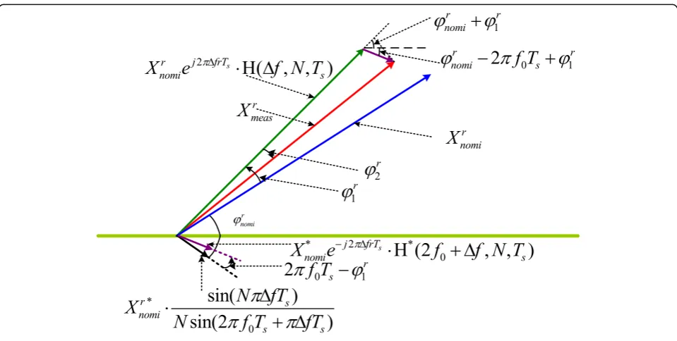
nomi¼φ0þ2πr=Nat time tr. The measured one isXr_meas¼Ar_measejφrmeas, and the mea-sured phasor Xr_measfor the off-nominal signal x(t) ac-cording to DFT is

Xr

constant (detail formula derivations are in Appendix); and symbol “*” denotes the conjugation of a complex number. shown in Fig.2and can be calculated as

φr

The measured phase angleφr_measis

φr

According to Eq. 7, for the first two phase angles cal-culated by DFT, we have

fr¼0 meas¼

φr¼1 meas−φrmeas¼0

2πTs ¼

φr¼1

nomiþφr1¼1−φr2¼1

− φr¼0

nomiþφr1¼0−φr2¼0

2πTs

¼φ1nomi−φ0nomi

2πTs þΔf−

Δf

2 sin 2ð πf0TsÞ

½sin 2φ1

nomiþ2φ11−2πf0Ts

−sin 2φ0

nomiþ2φ01−2πf0Ts

¼f0þΔf− Δf

sin 2ð πf0TsÞ

cos φ1nomiþφ

1 1þφ

0 nomiþφ

0 1−2πf0Ts

sinφ1

nomiþφ11−φ0meas−φ01

¼f0þΔf− Δf

sin 2ð πf0TsÞ

cos 2½ φ0þð2Nþ1ÞπΔfT_s

sin 2½ πð1þΔf=f0Þ=N:

ð13Þ

Without loss of generality, since N> > 4 and Δf< <f0,

and suppose φ0= 0, such in-equation of 0 < cos[(2N+

1)πΔfTs] < 1 can be fulfilled. We have

f0< fmeas≤f0þΔf; ifΔf≥0

f0þΔf≤fmeas< f0;ifΔf <0

ð14Þ

3 Frequency tracking by iterative DFT with re-sampling

3.1 Inner-layered DFT iteration by re-sampling

From analysis above, the measured frequency fmeas

would approach f0+Δf more and more closely if we

change the sampling frequency fs=Nfmeas consecutively.

Especially when the sampling frequency becomes closely enough to the value of N(f0+Δf), DFT calculated

itera-tively would give a measured frequencyfmeasas the input

and off-nominal frequency f0+Δfexactly. It means that

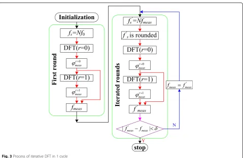
there are integral samples in 1 cycle of the input frequency again. The process of iterative DFT algo-rithm within 1 cycle (i.e., inner-layered iteration) is shown in Fig. 3.

In the first cycle of DFT calculation, the sampling fre-quencyfsis set to be Nf0and two phasor are calculated

to get the frequency fmeas. Then in the following cycle,

new f0_measis gotten according to the sampling frequency of f0_s¼Nf_meas, until difference of two successive fre-quencies f0_meas and fmeas is less than a threshold δ. In

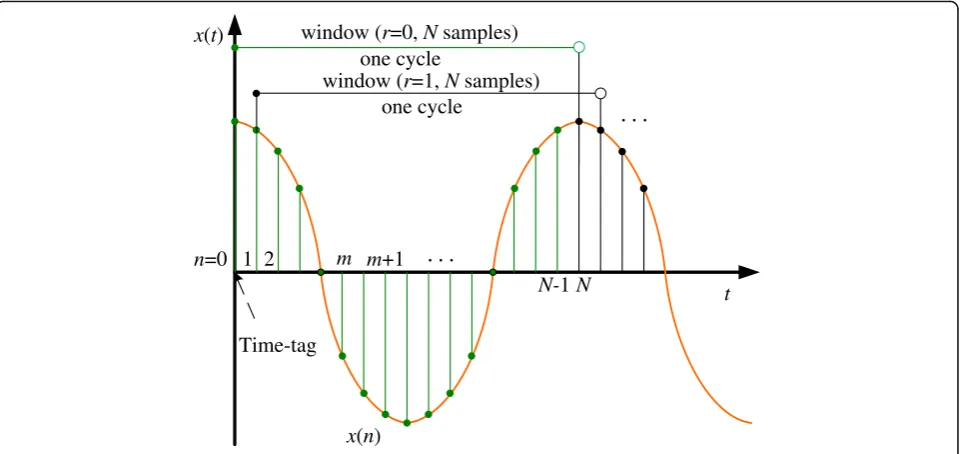
Fig. 4, samples are taken by a rectangular overlapping shifting window at timetr=rTs(r= 0 and 1 respectively)

as shown in Fig. 4. The first rectangle window contains Nsamples s0,s1,…,sN −1but not the sample of SN;

how-ever, the length of this window is N*Ts, whereTsis the

sampling period. In the second rectangle window, N samples s1,s2,…,sN are taken with the same lengthN*Ts

and so on.

3.2 Outer-layered DFT iteration between cycles

3.2.1 Determination of initial frequency by amended exponential sampling

In the dynamic states or under the circumstance of low signal-to-noise ratio (SNR), the input frequency may change in every cycle. It introduces lots of harmonics and spectrum leakage, and also limits the application of exponential sampling in such situation. Exponential sampling is a kind of simple frequency estimation algo-rithm, which can simplify the process of sampling by

ex-ponential sampling and need only few samples

distributed exponentially along the time [14]. Frequency is estimate based on a modified exponential sampling method, which is amended to be used in non-steady states.

For traditional exponential sampling, the sample are taken exponentially at

tp¼2p−Q−1 ð Þs ;p¼1;2;…;P; ð15Þ

wherePdefines the bit accuracy, andQdefines the max-imal frequencyfmax= 2Q. The samples are

x tp ¼Acos 2πftpþφ0

; ð16Þ

wherefis the instantaneous frequency attp, and it is not a constant anymore in the dynamic states. According to [14], the signal is a kind of sinusoidal signal. If a cosine

signal is used in accordance with Eqs. 1, 8, and 16, we have

s tp ¼

ffiffiffiffiffiffiffiffiffiffiffiffiffiffiffiffiffiffi

1−x tp 2

q

; ð17Þ

where symbols of“+”and“−”are taken according to the quadrants of phases of the signal. To guarantee the fre-quency to be an accuracy of 2Q−PHz, we get

fmeas¼ fmax

XP p¼1

bp2−p; ð18Þ

where

bp¼0; if s tp >0 bp¼1; if s tp <0

ð19Þ

If s(t_p) = 0 for somep=p0≤P, and bp0 ¼1, the Eq.18 is rewritten to be

fmeas¼ fmax

Xp0 p¼1

bp2−p; ð20Þ

where p0 is a terminator of exponential sampling. For

example, if a power system with a nominal frequency of 60 Hz and the dynamic frequency range is [−5, + 5] Hz, it indicates that off-nominal frequency may be 65 Hz > 64 = 26Hz. Hence, we setQ= 7 andP= 7 for an accuracy of 1 Hz. We getx(tp) = {−0.9809, 0.9239, 0.7071, 0,−1, 1, 1}, and let us supposeφ0= 0,s(tp) = {0.1951,−0.3827,−0.7071, −1, 0, 0, 0} and b= {0, 1, 1, 1, 1, 0, 0}, where p0= 5

without regard of noise.

window (r=0,Nsamples)

Time-tag

n=0 1 2 m m+1

N-1N

one cycle

x(n)

t x(t)

window (r=1,Nsamples)

one cycle

Two factors influence the accuracy or even the cor-rectness of frequency estimation by exponential sam-pling: first of all, if at the first sampling time t1= 1/128

(s), the system frequency is suddenly changed to 65 Hz, we have s(t1) =−0.0491, which means b1= 1 and

intro-duces frequency estimation error of 2Q−1= 64 Hz; sec-ondly, if the noise is big enough, values of samples may change from negative to positive (e.g.,b2=−0.3827 may

change to a positive value because of noise), which introduce frequency error of 2Q−2= 32 Hz. So in the algorithm of amended exponential sampling (AES), we may setb0= 0 andb1= 1 constantly forP=Q= 7.

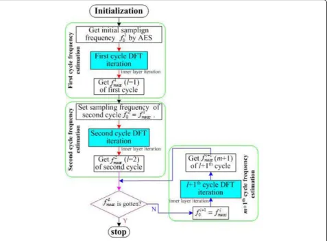
3.2.2 Process of frequency tracking cycle-by-cycle

Flow chart of DFT iteration is shown in Fig.5, where L is the total number of cycles to be generated and fl_meas, l= 1,2,…,L are the measured frequency in the lth cycle by inner-layered calculation. In the following, we named the algorithm as “TLI-DFT (Two-layered iterative DFT) aided by AES”. In Fig. 5, the inner-layered iteration

processes are implemented by iterative DFT in 1 cycle as shown in Fig.3.

3.2.3 Rate of change of amplitude and frequency

The rate of change of amplitude (ROCOA) is a simple technical analysis indicator showing the difference between the amplitudes of phasor Ar + 1 and Ar in the period ofTs. It is calculated by taking the time-derivative

of the estimated amplitude numerically

ROCOAð Þ ¼r Arþ1−Ar=Ts: ð21Þ And the rate of change of frequency (ROCOF) in electri-city networks is required by new IEEE/IEC/ CENELEC standards. Network frequency and its variation are key in-dicators of network stability and balance between electri-city supply and demand. This balance is becoming more critical with the increasing use of highly variable renewable energy sources for electricity generation. At the same time, ROCOF measurements are inadequate for monitoring this balance. The ROCOF is calculated by

ROCOFð Þ ¼r frþ1−fr=Ts : ð22Þ

3.3 DFT analysis of off-nominal stepped-signals

In general, voltage and current waveforms are not al-ways nominal sinusoids or cosine wave, particular in a distributed power system. Researchers have done some works on correcting this asynchronous effect [13, 28, 29]. Transients are non-unsteady states that occur in the power system. They are electrical tran-sients and electromechanical trantran-sients generally.

The former are caused by faults and other switching operations, while the latter ones are generated by dy-namic movement of rotors of generators and follow-ing power system disturbances [26, 30]. Phasors calculated in electrical transients often display a step change in phase angles and amplitude, but not the frequency. However, the motor speed in modern

power systems may deviate from synchronous speed by 0.1~5 Hz, the phase angle behavior during the phasor estimation window is approximately linear [26, 30]. Recommend by IEEE Std. C37.118-2005 [30], three step-changing models are adopted.

3.3.1 Scenario of amplitude step Signal of amplitude step is

xð0≤t<2TÞ ¼Acos 2ð πf₀tþφ₀Þ

x tð ¼2TÞ ¼AþA

0

2 cos 2ð πf0tþφ0Þ

xð2T <t<4TÞ ¼A0 cos 2ð πf₀tþφ₀Þ

8 > > < > >

: ; ð

23Þ

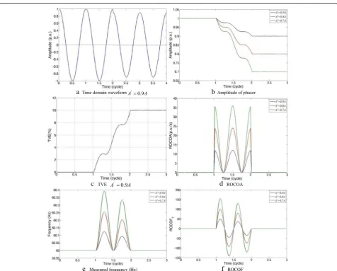
where A and A' (we haveA′∈{0.9A, 0.8A, 0.7A}) are the amplitudes of a voltage or current signal. An ex-ample of an amplitude step is shown in Fig. 6, in which A= 1 p.u.. A step change occurs (A’→A) at

Measured frequency (Hz) ROCOF

a b

c d

e f

time t= 2T (cycle) in Fig. 6a. Amplitude given by phasor is shown in Fig. 6b. The total vector error (TVE) accuracy criterion detects errors in time synchronization, and phasor magnitude and angle es-timation errors shown in Fig. 6c, where an amplitude variation of 0.1A generates 10% TVE.

TVE calculate the distortion of the signal from the nominal one by

TVE¼jXmeas−Xnomij jXnomij

100%; ð24Þ

where Xmeas is the measured vector, and Xnomi is the

nominal one.

The theoretical values of a synchrophasor representa-tion of a sinusoid and the values obtained from a PMU (phasor measure unit) may include differences in both amplitude and phase. Although they could be separately specified, the amplitude and phase differences are

considered together in this standard in the quantity called TVE. TVE is an expression of the difference be-tween a “perfect” sample of a theoretical synchrophasor and the estimate given by the unit under test at the same instant of time [25].

The amplitude step change can influence phase angle of a phasor, the measured frequency, and ROCOF.

ROCOA, ROCOF, and frequency calculated by trad-itional DFT algorithm is shown in Fig. 6c–e. We find that an amplitude step can influence phasor measure-ment whose samples contains the stepped one and the variation starts from the beginning of first cycle to be-ginning of second cycle (in time-axis) as shown in Fig.6.

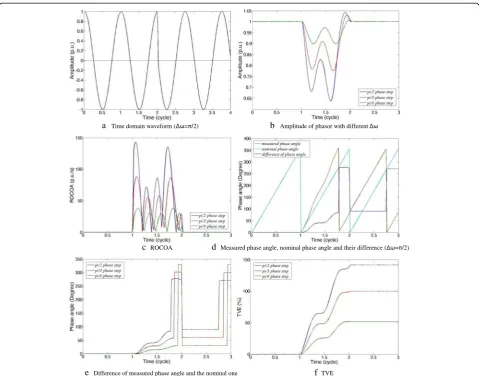
3.3.2 Scenario of phase step

A step change of phase angle Δω (Δω∈{π/2,π/3,π/6}) at timet= 2T(cycle) is shown in Fig.7, in whichA= 1 p.u.,f0= 60 Hz,φ0= 0. We have

Time domain waveform Amplitude of phasor with

ROCOA Measured phase angle, nominal phase angle and their difference

Difference of measured phase angle and the nominal one TVE

a b

c d

e f

xð0≤t<2TÞ ¼Acos 2ð πf₀tÞ

x tð ¼2TÞ ¼Acos 2ð πf₀tþΔω=2Þ

xð2T <t<4TÞ ¼Acos 2ð πf₀tþΔωÞ

8 <

: ð25Þ

Phase step influences amplitude and phase of measured phasor in a great deal. The measured TVE, frequency, and ROCOF are influenced as well as shown in Fig.7.

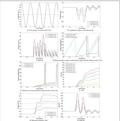
3.3.3 Scenario of frequency step The signal of frequency step is

xð0≤t<2TÞ ¼Acos 2ð πf₀tþφ₀Þ

x tð ¼2TÞ ¼A

xð2T <t<4TÞ ¼Acos 2ð πðf₀þΔfÞtÞ

8 <

: ; ð26Þ

whereΔfis the frequency step of the signal as shown in Fig. 8, in which A= 1 p.u., f

0= 60 Hz, and φ0= 0.

Step occurs at the beginning of the second cycle t= 2T (cycle).

A phasor is severely influenced by step frequency as long as it exists in the signal. The circumstances of

Time domain waveform (Δf=3 Hz) Amplitude of phasor with differentΔf

ROCOA Measured phase angle, nominal phase angle and their difference(Δf=3 Hz)

Difference of measured phase angle and the nominal one TVE

Measured frequency (Hz) ROCOF

a b

c d

e f

g h

phase step and frequency step are similar as shown in Figs.7and8.

4 Simulation results and data analysis

Traditionally, an adaptive sampling algorithm with vary-ing sample interval T_s is adopted. Based on a feedback system, if the sampling frequencyf_sequals toNtimes of the frequency of the incoming signal finput, it provides

that the incoming signal does not fluctuate in frequency [31]. New algorithm is compared with the traditional one. Parameters used in simulation are listed in Table1.

Weighted mean value of frequency f_r in Eq. 27 is adopted by iteration process.

fr¼0:6frþ2þ0:3frþ1þ0:1fr ðr≥0Þ: ð27Þ

Weighted mean of fr, fr + 1, and fr+ 2 that are

calcu-lated by three successive windows is adopted as a substi-tute of fr, which can provide a more smooth value for

evaluation [25].

Five more complicated scenarios are considered to demonstrate the performance of the algorithms in the following text.

Scenario 1: Frequency changes randomly in every cycle. The signal with frequency change randomly in each cycle is represented as

x tð Þ ¼Acos 2½ πðf₀þΔf_lÞtþφ₀ þNnoise l¼1;2;…;L;0≤t≤LT

ð Þ; ð28Þ

where Δfl= {Δf1,Δf2,…,ΔfL} and the integral Δfl∈[−5,

5]Hz are generated stochastically.

Sudden change of frequency introduces harmonics. Signals of this scenario contain additive white Gaussian noise (AWGN) Nnoise which can influence convergence

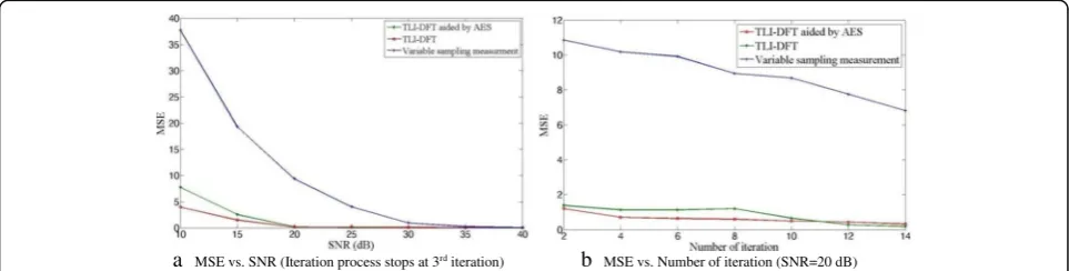
of DFT iteration, especially in the situation of low SNR. Results of frequency tracking cycle-by-cycle by three al-gorithms are listed in Table 2, in which the smallest MSE is gotten by TLI-DFT aided by AES. Mean squared error (MSE) of frequencies versus SNR and the number of iterations are shown in Fig.9.

Because Δfl is generated stochastically in every cycle,

frequencies of different cycles are irrelevant. Iterative DFT algorithm was utilized according to Fig.3.

Comparing with algorithm of DFT iteration (red curve) in 1 cycle, algorithm of“DFT aided by AES (Green curve)” would not do much help as shown in Fig. 9. It is due to the fact that frequency step happens at the beginning of every cycle randomly, and the frequency calculated in pre-vious cycle would not help to give a more precise initial frequency for the following cycle. In the algorithm of [31], the sampling frequency at each iteration is re-calculated till the value of tan(φm/2) approaching the nominal and

fixed value tan(φ0/2) [31].

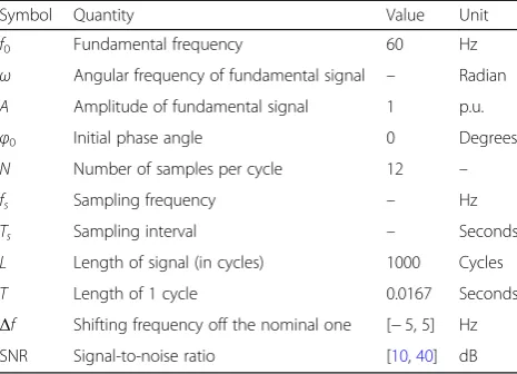
In each cycle of iteration, three measured frequencies are calculated by shifting windows, and then they are weighted and averaged by Eq. 27. Performance of DFT iteration is better than the traditional one. In Figs. 9aand 10a, MSE Table 1Parameters used in simulation

Symbol Quantity Value Unit

f0 Fundamental frequency 60 Hz ω Angular frequency of fundamental signal – Radian

A Amplitude of fundamental signal 1 p.u.

φ0 Initial phase angle 0 Degrees

N Number of samples per cycle 12 –

fs Sampling frequency – Hz

Ts Sampling interval – Seconds

L Length of signal (in cycles) 1000 Cycles

T Length of 1 cycle 0.0167 Seconds

Δf Shifting frequency off the nominal one [−5, 5] Hz SNR Signal-to-noise ratio [10,40] dB

Table 2Comparison of three algorithms (iterative process stops at third iteration)

SNR Algorithm Δfl(input frequency generated randomly per cycle, which are listed for the first 10 cycles, Hz) Total

MSE

1 2 3 4 5 6 7 8 9 10

0 (60) 0 (60) 5 (65) −3 (57) 2 (62) −2 (58) −2 (58) 4 (64) 0 (60) 1 (61)

20 dB DFT iteration aided by AES 60.0333 58.4136 64.0000 57.9770 60.6543 57.1513 57.5411 63.5073 58.9226 61.1667 1.9778

DFT iteration 59.2771 58.7789 65.5311 57.7068 60.6949 56.6914 57.1799 64.4430 59.3222 62.5303 1.4521

Variable sampling measurement [31] 57.4167 62.9167 62.7500 60.3333 61.0000 58.4167 60.2500 64.8333 55.7500 61.8333 5.5808

15 dB 3 (63) 2 (62) 5 (65) −3 (57) 4 (64) 0 (60) 2 (62) −4 (56) −3 (57) 5 (65)

DFT iteration aided by AES 64.0144 60.2727 62.6321 55.2965 60.7808 58.0518 65.3453 57.9144 58.0186 64.9271 3.8810

DFT iteration 63.6640 61.2829 57.7354 56.3717 65.5300 57.5044 62.4709 55.4884 56.9142 60.9407 3.6784

decreases with the increasing of SNR. In Figs.9band10b, the gain is 5.6~6 dB better than algorithm of [31] .

Scenario 2: Amplitude modulated by a cosine signal. The signal with amplitude modulated by a cosine sig-nal is represented as

x tð Þ ¼A½1þa cos 2ð πf_mtÞcos 2ð πf0tþφ0Þ þNnoiseð0≤t≤LTÞ;

ð29Þ whereaandfmare the modulating factor and the modula-tion frequency. Performances of three algorithms are compared and shown in Fig.10, from which we find per-formance of algorithm TLI-DFT aided by AES is better than other two if the SNR is less than 20 dB. And two or three times of iteration can give a satisfying result as shown in Fig.10b.

In Fig.11, MSE increases with the increasing offmand a. Using trigonometric function, Eq.29is rewritten to be

x tð Þ ¼Acos 2ð πf₀tþφ0Þ þNnoiseþAa

2 cos 2½ πðf0þfmÞtþφ0

þAa₂ cos 2½ πðf₀−f_mÞtþφ0 ð0≤t≤LTÞ:

ð30Þ

The amplitude modulation can be look on as adding inter-harmonics into a nominal signal from Eq. (30).

Because the modulation frequencyf_mis generally much smaller than the nominal frequency, the inter-harmonics are quite close to the nominal one in spectrum. It is hard

to be eliminated by low-pass filters (LPF) or smoothed by windows. Influence of inter-harmonics on TVE is shown in Fig.12with differentfmanda.

Scenario 3: Phase modulated by a cosine signal. The signal with phase modulated by a cosine signal is represented by

x tð Þ ¼Acos 2ð πf₀tþa cos 2ð πf_mtÞ þφ₀Þ þNnoise ¼Acos 2ð πf₀tþφ_mþφ₀Þ þNnoise;

ð31Þ

where a is modulation factor andfm is modulation fre-quency. Adopting second-order Taylor expansion and trigonometric function, we have

x tð Þ ¼Acos 2ð πf₀tþacos 2ð πf_mtÞ þφ₀Þ ¼

Taylor

Acos 2ð πf₀tþφ₀Þ−A2πf₀ sin 2ð πf₀tþφ₀Þ acos 2ð πf_mtÞ

−Að2πf₀Þ2 cos 2ð πf0tþφ0Þ

2! ½a cos 2ð πfmtÞ 2_þ… ≈Acos 2ð πf₀tþφ₀Þ−A2πf0a

2 sin 2½ πðf0þfmÞtþφ0

−A2πf0a

2 sin 2½ πðf0−fmÞtþφ0;

ð32Þ

where phase modulation factor a< < 1. The phase MSE vs. SNR (Iteration process stops at 3 iteration) MSE rd vs. Number of iteration (SNR=20 dB)

a b

Fig. 9Performance comparison of three algorithms in scenario 1 (in the first algorithm (red)), initial frequency estimation of DFT iteration is aided by AES, in whichP=Q= 7. In the second algorithm (green), initial frequency for DFT iteration is set to be 60 Hz in every cycle. The third one is from paper [31])

MSE vs. SNR (Iteration process stops at 3rd_{iteration) MSE vs. Number of iteration (SNR=20 dB)}

MSE vs. fm MSE vs. a

a b

Fig. 11Performance of TLI-DFT with or without AES algorithms in scenario 2 (iterative process stops at third iteration,a= 0.04,fm= 2 Hz)

Amplitude of phasor (fm=2 Hz) TVE (fm=2 Hz)

Amplitude of phasor (fm=4 Hz) TVE (fm=4 Hz)

Amplitude of phasor (fm=6 Hz) TVE (fm=6 Hz)

a b

c d

e f

modulation is the same as amplitude modulation in Eq. 30. And if the amplitude and phase modulations occur simultaneously, the signal x(t) contains the sum and difference frequencies of sine and cosine compo-nents, which is called inter-modulation. TVE of phasor in phase modulation with different modulation fre-quency is shown in Fig.13.

Scenario 4: Frequency modulated by a cosine signal. A signal whose frequency is modulated by cosine sig-nal with the modulation factor a and the modulation frequencyfmis represented as

x tð Þ ¼Acos 2ð πðf₀þa cos 2ð πf_mtÞÞtþφ₀Þ þNnoise ¼Acos 2ð πf₀tþa2πcos 2ð πf_mtÞtþφ₀Þ þNnoise ¼Acos 2πf₀tþφ0_mþφ₀

þNnoise;

ð33Þ

whose representation is the same as the representa-tion of Eq. 31, except φ0_m¼a2πcosð2πf_mtÞt. And the

φ0mwill become bigger and bigger with the passing of time t. Fortunately, three kinds of modulation in sce-nario 2~4 are all of short-time characteristic, which lasts only several cycles in transient states of a power system. So the representations of three modulation models are all similar in transient conditions.

Scenario 5: Decaying direct current offset components.

In an electrical power system, when a fault or a dis-turbance occurs, the current signal consists of expo-nentially decaying direct current (DC) offsets. The

decaying rate of a DC offset depends on the

time-constant determined by the inductive reactance to resistance ratio (X/R ratio) of the system. The large the X/R ratio is, the slower the DC component decays. Signal containing both the nominal compo-nent and decaying DC offsets is

x tð Þ ¼Acos 2ð πf0tþφ₀Þ−X NDC

i¼1

Iie−t=τiþNnoiseð0≤t≤TDCÞ;

ð34Þ

where NDC is the number of DC offset components, Ii and τi are the amplitude and time constant of the

ith DC offset component. TDC is the operation time

of decaying DC offsets. DC offset is a non-periodic signal whose frequency encompasses the whole spectrum, and it cannot be removed by simple anti-aliasing LPF.

fm=2 Hz fm=4 Hz

fm=6 Hz

a b

c

Fig. 13TVE of phasor in phase modulation with different modulating factor and modulation frequency (A= 1 p.u.,f0= 60 Hz,φ0= 0)

Table 3Parameters of decaying DC offset components

Number AmplitudeIi(p.u.) Time constantτi(cycle)

1 −1 0.5

A digital mimic filter was proposed to suppress the effect of decaying DC offsets over a broad range of time constants [32, 33]. But this filter needs exact values of the time constants for eliminating DC off-sets, which is usually impractical in power system. Kalman filter also needs the exact time constants to obtain a good performance of filtering [5–7, 34]. DFT-based techniques are generally used for removal decaying DC offset from phasor estimation [35–40]. On the other hand, the decaying DC component af-fects the accuracy of the DFT algorithm greatly [41– 43]. Different windows have been suggested and half-cycle DFT was used to get the phasor [10, 43– 45] in the case of decaying DC offsets. Full-cycle DFT is a widely adopted [33, 36, 46]. Suppose there are two decaying DC offset components (i.e., NDC=

2). Their parameters are listed in Table 3. Their wave-forms are shown in Figs. 14 and 15. Speed of decaying of DC offset 1 is faster than that of DC set 2. But the absolute value of amplitude of DC off-set 2 is smaller.

In Figs. 9, 10, and 16, SNR = 20 dB is about the point of inflection, although curves of MSE are not as smooth as desirable owing to the limitation of num-ber of estimated frequencies (i.e.,TDC= 10 cycle). MSE

of our proposed algorithms would not obtain much more gain when number of iterations is more than 3 or 4 as shown in Fig. 16b.

Frequency tracking and ROCOF by TLI-DFT are plotted in Fig. 17. Performance of algorithm TLI-DFT aided by AES is almost the same as that of TLI-DFT,

because AES is used only once in the initial

Fig. 14Waveform described in scenario 5

frequency estimation of inner-layered iteration in the first cycle.

5 Additional discussions

Chaari et al. proposed a new tool of wavelets for the resonant-grounded power distribution systems [47–49]. An earth-phase fault was simulated, and then a wavelet transform (WT) is applied on two kinds of fault currents in the transient signals. The meaningful information is contained in fault signals and was obtained by this re-cursive wavelet transformation.

They also used wavelets-associated artificial neural networks to classified fault currents. They chose “mother wavelet” by fast decaying oscillation function in a simulated 20 kV resonant grounded relaying networks.

According to WT theory, Zhang et al. constructed a mother wavelet that is suitable for processing transient signals in a power system [50]. WT was carried out to detect transform inrush current. This recursive WT con-sist of two parts: backward transform based on historical data and forward transform, the latter one is calculated with future data and is based on the detection of the singularity of the power signals.

WT is more suitable in detecting disturbances than

DFT/FFT when the time varies. With the

time-frequency localization characteristics embedded in wavelets, the information of frequency and time combined might be presented as a visualized scheme [51]. Morlet wavelets was adopted and tested of vari-ous simulated disturbances, e.g., harmonics analysis, momentary interruption and oscillatory, voltage swell, and sag. It is feasible and practical to use WT in supervising disturbances in a power system [52]; however, more suitable WT approaches should be found and evaluated.

Trapezoid WT was supposed to be better than other WT methods, such as Mexico hat wavelet, Haar wavelet, and Morlet wavelet, in localizability and sym-metry, and it had a more even frequency characteris-tics [53]. Trapezoid WT required less time-window data to detect characteristics in the fault signal and was better continuous than Shannon wavelet function in frequency tracking.

Lin et al. proposed a two-stepped approach to filter the high order harmonics by a bi-orthogonal WT and then extract the oscillation feature from the remnant signal by a complex WT. And in order to be imple-mented for real-time applications, they used a Mallat algorithm and the recursive version for torsional oscil-lation [54]. And furthermore, an improved boundary protection scheme based on a complex WT (which was MSE vs. SNR (Iteration process stops at 3rd_{iteration) MSE vs. Number of iteration (SNR=20 dB)}

a b

Fig. 16Performance of three algorithms with decaying DC offsets (considering the time constants of two decaying DC offsets.TDC= 10 cycle)

Frequency measured cycle-by-cycle ROCOF calculated cycle-by-cycle

a b

used as a band-pass filter to contain enough higher frequencies) and spectrum energy evaluation was put forward to distinguish internal faults from different kinds of external ones with higher reliability [55]. Their scheme provides an option to implement boundary pro-tection and transient-based propro-tection.

Within three samples of an input signal, a recursive WT was capable of estimating the frequency known as fast response. It also could achieve accurate esti-mation over a wide range of frequency changes [56– 58]. To meet the needs of high accuracy and low amount of calculation, people could select the signal sampling rate and data window length arbitrarily. In their conclusions, selecting sampling frequency of 18 kHz, a phasor could be computed within 0.5 cycle of input signal and the error was less than 1% TVE. How to select the two parameters of sampling rate and window length is the key issue.

6 Conclusions

A new approach of two-layered iterative DFT is proposed to track the input frequency in dynamic states. Inner-lay-ered DFT iteration is adopted in every cycle, and frequency estimated in the previous cycle is used as the initial frequency in the following one. And a simple and fast method, exponential sampling is amended to adapt to the non-steady states. This algorithm is more accurate than the traditional one. New algorithms are compared with the old one with different situations, e.g., input fre-quencies changing randomly, signal modulated by a cosine signal, and in the presence of decaying DC offsets. New algorithms are tested with different simulation parameters, such as different SNR and maximal numbers of iteration predefined to stop the iteration process.

Simulation results show that SNR of 20 dB is about the point of inflection. Low SNR would influence the performance of proposed algorithm. Fortunately, many researches show that wide-band AWGN is not a serious problem is power system, which is always more than 40 dB. And maximal numbers of iteration is better to be three or four. More iteration would not do much help to increase the accuracy of fre-quency estimation.

In practical, variable sampling algorithms are highly connected with phase locked loop (PLL) of the fre-quency generator and the digital signal processor.

Multiple-rated structure of adaptive PLL and

time-varying PLL-based sampling methods is the main work for implementation of the proposed TLI-DFT algorithm.

In the following study, Hamming window, Hanning window, Blackman window, and other kinks of win-dows should be compared with rectangle window used in this study.

Abbreviations

AES:Amended exponential sampling; AWGN: Additive white Gaussian noise; DC: Direct current; DFT: Discrete Fourier transform; FFT: Fast Fourier transform; LPF: Low-pass filters; MSE: Mean squared error; PLL: Phase locked loop; PMU: Phasor measure unit; ROCOA: Rate of change of amplitude; ROCOF: Rate of change of frequency; SNR: Signal-to-noise ratio; TLI-DFT: Two-layered iterative DFT; TVE: Total vector error; WT: Wavelet transform; X/R: Inductive reactance to resistance

Acknowledgements Not applicable

Funding

This work in partly supported by High Tech. of Key Research and Development Project of Hainan Province (ZDYF 2018012) and by National Natural Science Foundation of China (no. 61661018).

Authors’contributions

HL contributed 100%. The author read and approved the final manuscript.

Competing interests

The authors declare that they have no competing interests.

A small part of this paper was submitted to 2018 International Conference on Communications, Signal processing and Systems (CSPS 2018) previously. However, the vast majority of this study is original, and new algorithms and scenarios are introduced firstly in the paper. In this paper, a frequency estimation method named exponential sampling is amended to calculate the initial sampling frequency in the inner-layered process of the DFT iter-ation. Performance of new algorithm were studied and analyzed in some non-steady states of different scenarios (e.g., sudden and random frequency change, signal modulated by a cosine signal).

Publisher’s Note

Springer Nature remains neutral with regard to jurisdictional claims in published maps and institutional affiliations.

Received: 6 September 2018 Accepted: 11 December 2018

References

1. M.M. Begovic, P.M. Djuric, S. Dunlap, A.G. Phadke, Frequency tracking in power networks in the presence of harmonics. IEEE Trans. Power Del8(2), 480_–486 (1993)

2. C.T. Nguyen, K. Srinivasan, A new technique for rapid tracking of frequency deviation based on level crossings. IEEE Trans. Power App. SystPAS-103(8), 2230–2236 (1984)

3. M.S. Sachdev, M.M. Giray, A least error squares technique for determining power system frequency. IEEE Trans. Power App. SystPAS-104(2), 437–444 (1985)

4. V.V. Terzija, M.B. Djuric, B.D. Kovacevic, Voltage phasor and local system frequency estimation using Newton type algorithm. IEEE Trans. Power Del

9(3), 1368–1374 (1994)

5. H.C. Wood, N.G. Johnson, M.S. Sachdev, Kalman filtering applied to power system measurements for relaying. IEEE Trans. Power App. SystPAS-104(12), 3565–3573 (1985)

6. A. Routray, A.K. Pradhan, K.P. Rao, A novel Kalman filter for frequency estimation of distorted signals in power systems. IEEE Trans. Instrum. Meas51(3), 469–479 (2002)

7. E.M. Siavashi, S. Afshania, M.T. Bina, M.K. Zadeh, M.R. Baradar,Frequency estimation of distorted signals in power systems using particle extended Kalman filter(2nd Int. Conf. PEITS, Shenzhen, 2009), pp. 174–178 8. T. Lobos, J. Rezmer, Real-time determination of power system frequency.

IEEE Trans. Instrum. Meas46(4), 877_–881 (1997)

9. R. Vianello, M.O. Prates, C.A. Duque, A.S. Cequeira, P.M. da Silveira, P.F. Ribeiro,New phasor estimator in the presence of harmonics, DC-offset and interharmonics(14th ICHQ, Bergamo, 2010), pp. 1_–5

10. J.Z. Yang, C.W. Liu,A new family of measurement technique for tracking voltage phasor, local system frequency, harmonics and DC offset, IEEE PES Summer Meeting(IEEE, Seattle, 2000), pp. 1327_–1332

11. B. Zeng, Z.S. Teng, Y.L. Cai, S.Y. Guo, B.Y. Qing, Harmonic phasor analysis based on improved FFT algorithm. IEEE Trans. Smart Grid2(1), 51–59 (2011) 12. M. Karimi-Ghartemani, B. Ooi, A. Bakhshai, inInvestigation of DFT-based

phasor measurement algorithm. IEEE PES General Meeting (IEEE, Minneapolis, 2010), pp. 1–6

13. A.G. Phadke, J.S. Thorp, M.G. Adamiak, A new measurement technique for tracking voltage phasor, local system frequency and rate of change of frequency. IEEE Trans. on Power App. SystPAS-102(5), 1025–1038 (1983)

14. S. Kay, Simple frequency estimation via exponential samples. IEEE Signal Process. Lett1(5), 73–75 (1994)

15. H. Olkkonen, J.T. Olkkonen, Log-time sampling of signals: Zeta transform. Open J. Discrete Mathematics1(2), 62–65 (2011)

16. I. Sadinezhad, V.G. Agelidis, inExtended staggered undersampling synchrophasor estimation technique for wide area measurement systems. IEEE PES ISGT (IEEE, Perth, 2011), pp. 1–7

17. C. Rusu, P. Kuosmanen, Phase approximation by logarithmic sampling of gain. IEEE Trans. Circuits Syst. II Analog Digit. Signal Process50(2), 93_–101 (2003) 18. S. Trittle, F.A. Hamprecht, Near optimum sampling design and an efficient

algorithm for single tone frequency estimation. Digit. Signal Process19(4), 628–639 (2009)

19. C.S. Yen, Phase-locked sampling instruments. IEEE Trans. Instrum. Meas14(1/2), 64–68 (1965)

20. H. Karimi, M. Karimi-Ghartemani, M.R. Iravani, Estimation of frequency and its rate of change for applications in power systems. IEEE Trans. Power Del

19(2), 472–480 (2004)

21. R. Elasmi-Ksibi, H. Besbes, R. Lopez-Valcarce, S. Cherif, Frequency estimation of real-valued single-tone in colored noise using multiple autocorrelation lags. Signal Process90(7), 2303–2307 (2010)

22. P. Stoica, R.L. Moses, T. Soderstrom, J. Li, Optimal high-order Yule-Walker estimation of sinusoidal frequencies. IEEE Trans. Signal Process39(6), 1360–1368 (1991)

23. D. Hart, D. Novosel, H. Y, B. Smith, M. Egolf, A new frequency tracking and phasor estimation algorithm for generator protection. IEEE Trans. Power Del

12(3), 1064–1073 (1997)

Modulus of f,N,Ts) Modulus of H(2f0 f,N,Ts)

a b

24. A.G. Phadke, B. Kasztenny, Synchronized phasor and frequency measurement under transient conditions. IEEE Trans. Power Del24(1), 89–95 (2009)

25. IEEE Standard for Synchrophasors Measurement for Power Systems. IEEE Power & Energy Society. IEEE Std. C37.118.1-2011 (Revision of IEEE Std. C37. 118TM_{-2005). 2011}

26. K. Martin, D. Hamai, M.G. Adamiak, S. Anderson, M. Begovic, G. Benmouyal, G. Brunello, J. Burger, J.Y. Cai, B. Dickerson, V. Gharpure, B. Kennedy, D. Karlsson, A. G. Phadke, J. Salj, V. Skendzic, J. Sperr, Y. Song, C. Huntley, B. Kasztenny, E. Price, Exploring the IEEE Standard C37.118-2005 synchrophasors for power systems. IEEE Trans. Power Del23(4), 1805–1811 (2008)

27. S. Gomes, N. Martins, A. Stankovic, inImproved controller design using new dynamic phasor models of SVC_’s suitable for high frequency analysis. IEEE PES Transm. Distrib. Conf. Exhibi (IEEE, Dallas, 2006), pp. 1436–1444

28. K. Nakano, Y. Ota, H. Ukai, K. Nakamura, H. Fujita,Frequency detection method based on recursive DFT algorithm(14th PSCC, Sevilla, 2002), pp. 1_–7 29. M.H. Wang, Y.Z. Sun, A practical method to improve phasor and power

measurement accuracy of DFT algorithms. IEEE Trans. Power Del21(3), 1054_–1062 (2006)

30. IEEE Standard for Synchrophasors for Power Systems. IEEE Power Engineering Society. IEEE Std. C37.118-2005 (Revision of IEEE Std. 1344TM -1995). 2006

31. G. Benmouyal, An adaptive sampling-interval generator for digital relaying. IEEE Trans. Power Del4(3), 1602–1609 (1989)

32. G. Benmouyal, Removal of DC–offset in current waveforms using digital mimic filtering. IEEE Trans. Power Del10(2), 621–630 (1995)

33. C.S. Yu, A discrete Fourier transform-based adaptive mimic phasor estimator for distance relaying applications. IEEE Trans. Power Del21(4), 1839–1846 (2006) 34. A.A. Girgis, R.G. Brown, Application of Kalman filtering in computer relaying.

IEEE Trans. App. SystPAS-100(7), 3387–3397 (1981)

35. T.S. Sidhu, X. Zhang, F. Albasri, M.S. Sachdev, Discrete-Fourier transform-based technique for removal of decaying DC offset from phasor estimates. IEE Proc. Gen. Transm. Distrib150(6), 745–752 (2003)

36. V. Balamourougan, T.S. Sidhu, inA new filtering technique to eliminate decaying dc and harmonics for power system phasor estimation. IEEE Power India Conf (IEEE, New Delhi), p. 2006

37. D. Belega, D. Petri, inAccuracy of a DFT phasor estimator at off-nominal frequency in either steady state of transient conditions. IEEE Int. Conf. SMFG (IEEE, Bologna, 2011), pp. 45–50

38. S.H. Kang, D.G. Lee, S.R. Nam, P.A. Crossley, Y.C. Kang, Fourier transform-based modified phasor estimation method immune to the effect of the DC offsets. IEEE Trans. Power Del24(3), 1104–1111 (2009)

39. D.G. Lee, Y.J. Oh, S.H. Kang, B.M. Han, inDistance relaying algorithm usinga DFT-based modified phasor estimation method. IEEE Bucharest Power Tech. Conf (IEEE, Bucharest, 2009), pp. 1–6

40. A.D. de Oliveira, L.R.M. Silva, C.H. Martins, R.R. Aleixo, C.A. Duque, A.S. Cerqueira, inAn improved DFT based method for phasor estimation in fault scenarios. IEEE PES General Meeting (IEEE, San Diego, 2012), pp. 1–5 41. H.B. ElRefaie, A.I. Megahed, inA novel technique to eliminate the effect of

decaying DC component on DFT based phasor estimation. IEEE PES General Meeting (IEEE, Minneapolis, 2010), pp. 1–8

42. Y.H. Lin, C.W. Liu, inA new DFT-based phasor computation algorithm for transmission line digital protection. Asia Pacific IEEE/PES Transm. Distrib. Conf. Exhibi (IEEE, Yokohama, 2002), pp. 1733–1737

43. X. Liu, M. Jia, X. Zhang, W. Lu, A novel multi-channel internet of things based on dynamic Spectrum sharing in 5G communication. IEEE Internet Things J. (Early Access)99, 1–1 (2018)

44. X. Liu, F. Li, Z.Y. Na, Optimal resource allocation in simultaneous cooperative Spectrum sensing and energy harvesting for multichannel cognitive radio. IEEE Access5, 3801–3812 (2017)

45. G. JC, Y. SL, Removal of DC offset in current and voltage signals using a novel Fourier filter algorithm. IEEE Trans. Power Del15(1), 73–79 (2000) 46. X. Liu, M. Jia, Z.Y. Na, W. Lu, F. Li, Multi-modal cooperative Spectrum sensing

based on Dempster-Shafer fusion in 5G-based cognitive radio. IEEE Access

6, 199–208 (2018)

47. M. Kezunovic, P. Spasojevic, B. Perunicic, New digital signal processing algorithms for frequency deviation measurement. IEEE Trans. Power Del

7(2), 1563–1573 (1992)

48. O. Chaari, M. Meunier, inA recursive wavelet transform analysis of Earth fault currents in Petersen-coil-protected power distribution networks. IEEE-SP

international symposium on time- frequency and time-scale analysis (IEEE, Philadelphia, 1994), pp. 162_–165

49. O. Chaari, M. Meunier, F. Brouaye, Wavelets: A new tool for the resonant grounded power distribution system relaying. IEEE Trans. Power Del11(3), 1301–1308 (1996)

50. C.L. Zhang, Y.Z. Huang, X.X. Ma, W.Z. Lu, G.X. Wang, inA new approach to detect transformer inrush current by applying wavelet transform. International Conference on Power System Technology. Proceedings (IEEE, Beijing, 1998), pp. 1040–1044

51. S.J. Huang, C.T. Hsieh, C.L. Huang, Application of Morlet wavelets to supervise power system disturbances. IEEE Trans. Power Del14(1), 235–243 (1999) 52. O. Poisson, P. Rioual, M. Meunier, inDetection and measurement of power

quality disturbances using wavelet transform. 8th International Conference on Harmonics and Quality of Power (IEEE, Athens, 1998), pp. 1125_–1130 53. Z. Ren, Q.G. Huang, L. Guan, W.Y. Huang, inA new method for power systems

frequency tracking based on trapezoid wavelet transform. 5th APSCOM (IEEE, Hongkong, 2000), pp. 364–369

54. X.N. Lin, H. Zhang, P. Liu, O.P. Malik, Wavelet based scheme for detection of torsional oscillation. IEEE Trans. Power Sys17(4), 1096–1101 (2002) 55. X.N. Lin, H.F. Liu, inA fast recursive wavelet based on boundary protection

scheme. IEEE Power Engineering Society General Meeting (IEEE, San Francisco, 2005), pp. 1_–6

56. J. Ren, M. Kezunovic, inUse of recursive wavelet transform for estimating power system frequency and phasors. IEEE PES T&D (IEEE, New Orleans, 2010), pp. 1–6

57. J. Ren, M. Kezunovic, inA wavelet method of power system frequency and harmonic estimation. North American Power Symposium (IEEE, Arlington, 2010), pp. 1–6