An Adaptive Channel Estimation Algorithm Using
Time-Frequency Polynomial Model for OFDM with
Fading Multipath Channels
Xiaowen Wang
Wireless Systems Research Department, Agere Systems, Murray Hill, NJ 07974, USA Email: [email protected]
K. J. Ray Liu
Electrical and Computer Engineering Department, University of Maryland, College Park, MD 20742, USA Email: [email protected]
Received 1 August 2001 and in revised form 7 March 2002
Orthogonal frequency division multiplexing (OFDM) is an effective technique for the future 3G communications because of its great immunity to impulse noise and intersymbol interference. The channel estimation is a crucial aspect in the design of OFDM systems. In this work, we propose a channel estimation algorithm based on a time-frequency polynomial model of the fading multipath channels. The algorithm exploits the correlation of the channel responses in both time and frequency domains and hence reduce more noise than the methods using only time or frequency polynomial model. The estimator is also more robust compared to the existing methods based on Fourier transform. The simulation shows that it has more than 5 dB improvement in terms of mean-squared estimation error under some practical channel conditions. The algorithm needs little prior knowledge about the delay and fading properties of the channel. The algorithm can be implemented recursively and can adjust itself to follow the variation of the channel statistics.
Keywords and phrases:channel estimation, OFDM, polynomial approximation.
1. INTRODUCTION
The 3G wireless communication system is the next genera-tion mobile cellular system that aims to provide high rate data communications of a bit rate up to 2 Mbit/s. Among many technical challenges in this broadband system, the se-vere intersymbol interference (ISI) caused by multipath ef-fect of wireless channels is an essential one. One effective technique to deal with this problem is the orthogonal fre-quency division multiplexing (OFDM) [1, 2]. In OFDM sys-tems, the entire bandwidth is partitioned into parallel sub-channels by dividing the transmit data into several paral-lel low bit rate data streams to modulate the carriers cor-responding to those subchannels. By doing so, the OFDM system has a relatively longer symbol duration, thus pro-vides a great resistance to ISI and impulse noise. When the number of subchannels is large enough, the subchannels can be treated as independent of each other and only a one-tap equalizer is needed for each subchannel. Because of these advantages, OFDM has become a promising technique for broadband wireless communications.
Channel estimation is a key issue in a communication
system, as is the case for the OFDM system. Without the knowledge of channel information, noncoherent detection, such as differential modulation, has to be used and results in some performance loss compared to the coherent detec-tion. The channel estimation problem becomes more im-portant for the 3G systems because many sophisticated sig-nal processing techniques that require the knowledge of the channel information are expected to be used to meet the challenge of throughput and performance. For example, the independence of the subchannels in OFDM systems pro-vides an easy way to optimize the transmitter design by adjusting the bit rate and transmit power across subchan-nels according to their channel conditions [3], which im-plies that the channel information has to be known at the transmitter.
independently when performing the signal detection. The channel estimation algorithms should exploit such correla-tion to improve the accuracy of the estimacorrela-tion. Van de Beek et al. [4] tried to exploit the correlation of the channel pa-rameters in frequency domain while Mignone and Morello [5] used the correlation in time domain. Li et al. [6] con-sidered the correlation in both time and frequency domains. The estimators designed in these literatures are all Fourier-transform-based approaches, which implicitly assumed that the channel power spectrum can be viewed as band lim-ited. The assumption is true when we consider the ensemble statistics. However, in practice, we can only get finite discrete samples of the channel response of the time varying channel. The leakage can be very severe and then degrade the perfor-mance dramatically.
In this work, we consider the problem from another point of view. Because of the correlation of the fading multi-path channel, it can be viewed as a smoothly varying function of both time and frequency. It has been stated in the approx-imation theory that such a smoothly varying function can be approximated by a set of basis functions [7], for example, the polynomial basis [8]. Borah and Hart [9, 10] used the time domain polynomial approximation while Luise et al. in [11] used the frequency domain polynomial approximation. However, the channel responses used in coherent detection of OFDM are located in the time-frequency plane. Therefore, it is naturally to exploit the channel correlation in both time and frequency domains using a time-frequency polynomial model. The noise can then be greatly suppressed by estimat-ing a smaller number of coefficients of the basis functions over a large number of observations. Moreover, it also make the estimator design more flexible and robust to the variation of channel statistics. We can also view Fourier transform as a type of model basis function and hence Fourier-transform-based method is the same type of method as the polynomial-model-based channel estimation scheme but with diff er-ent model accuracy and different noise reduction capability. These two methods compared, the model error of the Fourier basis is very sensitive to the channel statistics and works only for some very specific system parameters and channel statis-tics. On the contrary, the polynomial-model-based method performs more consistently and robustly for variety of channels.
A key problem in using the polynomial model to estimate the channel responses is to decide the model order and time-frequency window dimensions of observations. The model approximation error of polynomial model decreases when increasing model order or decreasing the window dimen-sions. On the other hand, the noise is reduced more when decreasing the model order or increasing the window dimen-sions. It is important to reach a tradeoffbetween the model error and noise reduction. In this paper, we propose an adap-tive algorithm that adjusts the window dimensions to balance the tradeoff. With this adaptive algorithm, the channel corre-lation function or the fading and delay characteristics are no longer that essential in the design of the channel estimator. The estimator can adapt its settings to the variation of the channel statistics.
Figure1: OFDM transmitter and receiver. (a) Transmitter, (b) re-ceiver.
The rest of the paper is organized as follows. First, we introduce the OFDM system in Section 2 and the fad-ing multipath channel in Section 3.1. Then, we discuss the time-frequency polynomial model Section 3.2 and de-rive the corresponding recursive channel estimation algo-rithm in Section 4. The performance analysis is discussed on the general-model-based estimation approach in Section 5. Then the window dimension adaptive algorithm is derived in Section 6 based on the performance analysis. Finally, the simulation results are presented to demonstrate the perfor-mance in Section 7 and the conclusion is drawn in Section 8.
2. OFDM SYSTEMS
Figures 1a and 1b show the transmitter and receiver of an OFDM system, respectively. The OFDM system divides the whole bandwidth Bd into m subchannels by buffering the
input data to blocks, and then partitions the block into m lower rate bit streams. In most of OFDM systems, the sub-channels are divided evenly, the bandwidth of the subchan-nels or the rate of the bit streams is ∆f = Bd/m. The bit
streams may contain different amount of bits and use dif-ferent transmit energy according to the channel condition. The bit and energy allocation is done by a loading algorithm. Then the bit streams are mapped to some complex constella-tion pointsXi,k, i=0, . . . , m−1 at thekth block. The
modula-tion is then implemented bym-point inverse discrete Fourier transform (IDFT). Then the modulated data go through P/S converter to form the serial dataxi,k. A cyclic prefix which is
constructed using the lastvsamples ofxi,k’s is inserted before
sending thexi,k’s to the channel. Now it follows that the
−1 0 1 2 3 4 5 6 t(µs)
0 0.1 0.2 0.3 0.4 0.5 0.6 0.7 0.8 0.9 1
Po
w
er
(a)
−2 0 2 4 6 8 10 12 14 16 18
t(µs) 0
0.1 0.2 0.3 0.4 0.5 0.6 0.7 0.8 0.9 1
Po
w
er
(b)
Figure2: Two typical delay profiles (a) TU and (b) HT.
Tf =(m+v)/Bd. For a system withBd=800 kHz,m=128,
andv =16, the block duration isTf = 180 microseconds.
Such a system is used in the rest of this paper.
At the receiver, the prefix part is discarded. The demodu-lation is performed by the discrete Fourier transform (DFT) operation. If the cyclic prefix is long enough, then the in-terference between two OFDM blocks is eliminated and the subchannels can be viewed as independent of each other, that is, the demodulated dataYi,kcan be expressed as
Yi,k=Hi,kXi,k+Ni,k, (1)
whereHi,k is the channel frequency response ati∆f ofkth
block andNi,kis the corresponding channel noise that is
as-sumed to be white Gaussian process with zero mean and vari-anceσ2.
Because of the simple relation of (1), only a one-tap equalizer is needed for each subchannel at the receiver, that is,
ˆ
Xi,k=Yi,kWi,k, (2)
where the equalizer coefficientWi,kis some function ofHi,k.
For example, the zero-forcing equalizer is constructed as Wi,k =1/Hi,k.Then the decision or decoding is made upon
ˆ Xi,k.
3. POLYNOMIAL CHANNEL MODEL 3.1. Fading multipath channel
In a mobile broadband wireless communication system such as 3G, the transmission is impaired by both fading that is due to the mobility, and multipath that is due to the wide band-width. This fading multipath channel has long been known to be modeled as a time-varying linear filter [12],
h(t, τ)=
i
γi(t)δ
τ−τi
, (3)
where γi(t)’s are independent complex Gaussian processes
with zero mean and variance pi’s. For OFDM systems, we
can assume that the channel is time varying for different blocks but time-invariant within one block. The channel fre-quency responseHi,k’s are samples of the continuous channel
responseH(t, f)=h(t, τ)e−j2π f τdτ, that is,
Hi,k=H
kTf, i∆f
. (4)
The correlation function ofH(t, f) is defined asrH(t, f)=
E[H(t1, f1)H∗(t1−t, f1− f)]. Assume that the correlation function ofγi(t) follows E[γi(t1)γi∗(t1−t)]=pir(t), then we
have
rH(t, f)=rt(t)rf(f). (5)
For the Rayleigh fading channel [12],rt(t)=J0(2π fDt) and
rf(f) =
ipie−j2π∆f τi with J0(·) denoting the zero-order Bessel function, fD being the Doppler frequency describing
the channel variation alongt, and pi’s together withτi’s
be-ing delay profiles describbe-ing the channel dispersion which is also often characterized by the maximum delay spread
Td = maxiτi. Three types of delay profiles are used in this
work, TU, HT, and 2-ray [13]. The TU and HT delay profiles are shown in Figure 2. The 2-ray delay profile has two equal power paths and the delay between two paths isTd. We also
assume that the channel is normalized in our simulation, that is,ipi=1.
From (5), the power spectrum of the channel response is
SH(ξ, ν)= rH(t, f)e−j(tξ+f ν)dξ dν=St(ξ)Sf(ν), (6)
where St(ξ) =
rt(t)e−jtξdξ andSf(ν) =
rf(f)e−j f νdν.
concen-trated in a finite bandwidth in both time and frequency do-mains. The bandwidths are fDforSt(ξ) andTdforSf(ν),
re-spectively.
3.2. Time-frequency polynomial channel model of OFDM systems
We know from the approximation theory [7, 8] that the smoothly varying channel responses can be approximated by projecting to a finite set of basis functions. In [14], it was shown that the channel responses in a small time domain window around a center pointk0 of dimension 2K+ 1 can be closely approximated by a small set of polynomial basis functions, that is,
For such an approximation, it can be proved that the mean-squared model error is bounded by
E RM 2
(10) that the sufficient condition for this error to con-verge to zero is fDTf 1, that is, if fDTf 1 then
limM→∞ E[RM2]= 0.
Similarly, if the channel delay spreadTdsatisfiesTd∆f
1, which means that the frequency variation of Hi,k’s is
smooth enough along frequencies, thenHi,k’s in a frequency
domain window of dimension 2I+ 1 aroundi0, [i0−I, i0+I], can be approximated by the polynomial bases, that is,
Hi,k=
The mean-squared model error of this approximation is bounded by
The time domain expansion (7) is used for channel esti-mation in [10], while the frequency domain expansion (10) is adopted in [11]. For a given channel, the selection of the above two types of expansions depends on the channel statis-tics, fD and Td, and the system parameters, Tf and ∆f.
Moreover, it is naturally to expand the channel responses in both time and frequency domains [15] for the OFDM sys-tem, since its signal is distributed in a time frequency plane. The expansion in the time-frequency window of dimensions (2I+ 1)×(2K+ 1) aroundi0andk0is
The mean-squared model error is then bounded by
E RMN 2
Without loss of generality, assuming M = N and us-ing the multipath Rayleigh fadus-ing channel described in Section 3.1, we can show that [15]
E RMM 2
Again the sufficient conditions for convergence of the above expansion are fDTf 1 and Td∆f 1. It is noticed
1 2 3 4 5
Bound on model error Residual noise (10 dB) Residual noise (20 dB)
Figure3: Bound on mean-squared model error.
OFDM systems. When fDTf > 1, the block duration is so
long or the channel changes are so fast that the channel can-not be viewed as invariant during one block and the system suffers large interchannel interference (ICI). On the other hand, whenTd∆f >1, the block duration is so short or the
channel dispersion is so large that the subchannels can no longer be treated independently and the system would suffer both ISI and ICI. The OFDM system cannot work in either case. Hence, it is reasonable to assume that both conditions are satisfied in a well designed OFDM system.
Now we take a close look at the upper bound of the model error. Suppose that the length of the cyclic prefixvcan be ig-nored compared to the number of the subchannels. Then the first term in (16) is determined by fDTf =m fD/Bd, while the
second term is determined by∆f Td = BdTd/m. The third
term is actually determined by fDTd and is much smaller
than the first two terms, since they both are smaller than one. For the first two terms, whenmis large, the first term is dominating, then we should choose smallerKor largerM. Whilemis small, then the second term is dominating and I should be smaller or the model orderN should be larger. If the Doppler frequency fD, maximum delayTd, and
band-widthBdare fixed, we can adjust the window dimensions
ac-cording tomto keep the time-frequency model error to cer-tain level but we still have a smallMN/IK. However, if only time or frequency domain expansion is used, the model error cannot be adjusted to maintain a small level with the same M/KorN/Iwhen the number of subchannelsmvaries.
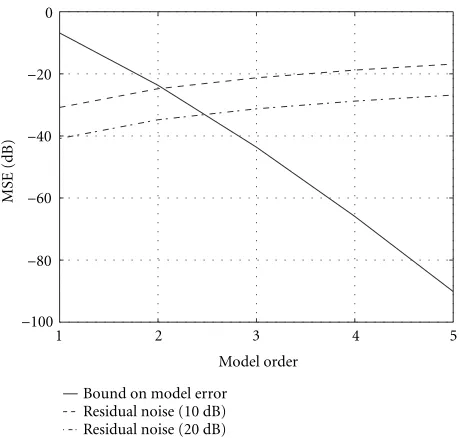
Figure 3 shows the upper bound of mean the squared model error with fDTf = Td∆f = 10−2 andI = K = 5
according to model orderM. It shows that the model error is under −40 dB as the model order is 3. This means that we only need to estimate 9 model coefficients to get the 121 channel responses. In this figure, we also show the residual noise for SNR of 10 dB and 20 dB. It shows that the noise
can be greatly reduced with very small penalty on model er-ror. Moreover, such a model approximation does not need to know the actual channel correlation function.
4. CHANNEL ESTIMATION ALGORITHM WITH POLYNOMIAL MODEL
4.1. Estimator structure
The channel estimation problem in OFDM systems is to es-timate the channel responseHi,k based on the transmitted
signalXi,k and the received signalYi,k. The information of
the transmitted signalXi,k’s is obtained either from training
or from detected feedback. In OFDM systems, an instanta-neous estimate can be easily constructed as ˜Hi,k =Yi,k/Xi,k.
Then suppose that we have chosen the model order and win-dow dimensions such that the model error is small and can be ignored, we can approximate (13) in a matrix form
Using least square (LS) methods, we can get the estimation of the coefficients of the polynomial basis from the instanta-neous estimates
channel estimation then can be constructed as
ˆ point of estimation inside the window and slide the window to get all the estimations. Then the estimator can be viewed as a two-dimensional filtering process. Arranging the instan-taneous estimation inside the window into a matrix form,
˜
Then the estimation is
ˆ
The estimator structure is shown in Figure 4. The coefficients of the frequency domain filter are Q†N(I)qN(i−i0) and the coefficients of the time domain filter areQ†M(K)qM(k−k0). 4.2. Recursive algorithms
The two-dimensional filter can actually be implemented re-cursively in time and frequency domains, respectively.
Define the basis functionsQN(I) as each other, that is, there is an invertible matrixRsuch that
QN(I)=QN(I)R. (29)
P/S domain filterTime
Reset every 2K+ 1 samples
ˆ Hi,k
Figure4: The estimator structure.
qTNi+ 1−i0
Q†N(I)=qTNi−i0
Q†N(I). (30) Substitute (30) into (26), we can estimate the channel using Q†n(I). Then the core of the recursive algorithm is to calcu-lateQ†N(I) fromQ†N(I) iteratively.
LetPf =(QTN(I)QN(I))−1andPt =(QTM(K)QM(K))−1.
At initialization, we estimate model coefficients ˆbf(k) or
ˆ
bt(i) regarding toPforPtover a window of dimension 2I+1
or 2K+ 1. Similar to the recursive least square (RLS) algo-rithm, using thematrix inverse lemma[16], we can calculate P+f =(QTN(I+ 1)QN(I+ 1))−1orP+
during theupdating process. After that apply thematrix in-verse lemmaagain, we can calculateP−f =(QTN(I)QN(I))−1 orP−t =(QTM(K)QM(K))−1and the corresponding model coefficients ˆb−f or ˆb−t fromP+
f orP+t over the window of
di-mension 2I+ 1 or 2K+ 1 during thedowndating process. Then according to (30), the channel can be estimated as
ˆ
As this recursive process going on, the basis function be-comesqT
M(k+l−k0) wherelis the index of the iteration. The dynamic range of such a basis function may become so large that it will affect the numerical stability of the algorithm. Therefore, regularization usingRf orRtshould be used
pe-riodically to scale the basis back to QN(I) orQM(K). The
frequency domain and time domain recursive algorithms are summarized in Algorithms 1 and 2, respectively. The matri-cesK+f andK−f orK+t andK−t are the correspondinggain
ma-tricesin updating and downdating. The two-dimensional fil-ter in the tables is implemented first by frequency domain filtering then by time domain filtering. The order can be switched. In that way, the input in Algorithm 2 are instanta-neous estimates while the inputs in Algorithm 1 are the out-puts of the time domain filters of Algorithm 2. It is also noted that the order of downdating and updating can be switched, too.
In both tables,K+
Initialization:
with temporary estimation ˜Hk= ˜
Algorithm1: Frequency domain recursive algorithm.
calculated off-line and do not change if the model order and window dimensions do not change. However, we still put the calculations inside the updating and downdating process in case that the window dimensions may change as what hap-pened in the adaptive algorithm described in Section 6.
The recursive algorithm needs less calculation compared to direct computation of the product of pseudoinverse when the window dimensions are much larger than the model or-der. Many fast algorithms of recursive least square (RLS) can be used for the practical implementation of such a recursive algorithm [16]. It also provides an easy way to adjust the win-dow dimensions for the implementation of the adaptive algo-rithm.
5. PERFORMANCE ANALYSIS
Suppose that the channel can be modeled by some basis func-tion, that is, a set of channel responsesHcan be projected to a set of basis functionQand the coefficients of the basis func-tions areb, that is,
H=Qb. (32)
The length ofHisLand the length ofbisl. In order to get an accurate channel estimation, we expect thatl L. This is true if the channel parameters in His highly correlated.
Initialization:
with frequency domain filter results ˆ
Algorithm2: Time domain recursive algorithm.
Given a set of noisy observations,
˜
H=H+N, (33)
the LS estimation of the coefficients is
ˆ
b=Q†H˜. (34)
The channel estimation is then
ˆ
H=QQ†H˜. (35)
Define the mean-squared estimation error matrix as
ε= EHˆ −HHˆ −HH. (36) We can show that
ε=I−QQ†RH
I−QQ†+QQ†RNQQ†, (37)
whereRH=E[HHH] andRN =E[NNH]=σ2Iif the
trans-mitted signals of all subchannels are all using the same con-stant envelop modulation and transmit energy of 1.
The estimation error consists of two parts; one is related to the model inaccuracy, that is,
εH=
I−QQ†RH
and the other is related to the residual noise, that is,
εN =σ2QQ†. (39)
SinceRHis a Toeplitz matrix, it can be decomposed as
RH=
whereΛis a diagonal matrix with eigenvalues ofRHon its
di-agonal. IfQ=U1, then the model error is zero. This means that the optimal function basis, which we can find in terms of model accuracy, is the eigenbasisU1. However, it requires the knowledge about the statistics of the channel responses. In some special cases, we can easily find some specific func-tion bases that can diagonalizeRHwithout actually knowing
RH. For example, ifHis the channel response for one OFDM
block with all the delay paths,τi’s, at the sampling instance of
the OFDM system, then such an optimal function basis is the DFT matrix [6]. However, in most of practical situations, the channel delay profiles do not satisfy this condition. There-fore, using DFT matrix may cause severe leakage problem and incur a large model error.
The average energy of the residual noise over the entire estimation window can be calculated as follows:
¯
The average mean-squared error over the whole estimation window is actually lower bounded by (41). The lower bound is achieved whenQ=U1.
Although the average energy of the residual noise main-tains the same once the data length and model order is fixed, the estimation error inside the window is often distributed unevenly and differently for different basis functions. For the polynomial model, the estimation error is the least at the cen-ter point of the window and larger at the edge. Therefore, we prefer to choose the center of the window to get a better performance. However, along the time domain, we can only choose the end point to get a causal filter.
6. OPTIMAL MODEL PARAMETERS ADAPTATION With estimation point chosen at the center of the frequency domain window and end point at the time domain window, the estimation error from (23) becomes
I,K=E Hi0,k0−Hˆi0,k0
2
=h+n, (42)
where the model error is
h=E Hi0,k0−qM,N(0, K)TQ
(1) Initialization: useI0×K0 calculate estimation and ˆ
0=ˆI0,K0.
(2) Use window dimensionsI×K to estimate thekth block and compute the estimated estimation error
ˆ
Algorithm3: Window dimension adaptive algorithm.
and the residual noise is
n=σ2qM,N(0, K)TQ†M,N(I, K)Q†M,NT (I, K)qM,N(0, K). (44)
The residual noise is reduced more when the model or-derM×Nbecomes small or the window dimensionI×K becomes large. However, the model error will increase in this case. With fixed polynomial model orderMandN, the opti-mal window dimension is obtained by
min
I,K I,K =h+n. (45)
Usually, there are several local minima in this optimiza-tion problem. Considering the computaoptimiza-tional complexity, we would prefer the one with smallI×K.
In order to adaptively adjust the window dimensions we need to know the estimation error. Since the actual chan-nel responses are not known, we have to estimate the esti-mation error using the instantaneous estimates and the final estimates. Suppose that the noise statistics is known, we can calculate the estimated estimation error as
ˆ
Using this approximation, the window dimension adap-tive algorithm for the optimization of (45) is given in Algorithm 3.
If the recursive algorithm in Algorithms 1 and 2 is adopted, the window adaptation can be implemented easily. We just eliminate one downdating when increasing the win-dow dimension, or eliminate one updating when decreasing window dimension.
0 5 10 15 20 25 30 SNR (dB)
−40
−35
−30
−25
−20
−15
−10
−5 0
MSE
(dB)
Polynomial approximation in time-frequency Polynomial approximation in time only Polynomial approximation in frequency only
(a)
10 12 14 16 18 20 22 24 26 28 30
SNR (dB) 10−3
10−2 10−1
SER
Polynomial approximation in time-frequency Polynomial approximation in time only Polynomial approximation in frequency only
(b)
0 5 10 15 20 25 30
SNR (dB)
−40
−35
−30
−25
−20
−15
−10
−5
MSE
(dB)
Polynomial approximation in time-frequency Polynomial approximation in time only Polynomial approximation in frequency only
(c)
10 12 14 16 18 20 22 24 26 28 30
SNR (dB) 10−3
10−2 10−1
SER
Polynomial approximation in time-frequency Polynomial approximation in time only Polynomial approximation in frequency only
(d)
Figure5: Estimation error and symbol error rate versus SNR (2-ray,M×N =3×3) (a) MSE, (b) SER (fD=40 Hz,Td=5 microseconds,
I×K=7×10), (c) MSE, and (d) SER (fD=20 Hz,Td=10 microseconds,I×K=4×30).
large threshold may result in unstable convergence. Hence, it would be preferred to use smaller thresholds here.
7. SIMULATION RESULTS
The OFDM system used in the simulations is the system in-troduced in Section 2. QPSK modulation is used throughout all subchannels. Figure 5 shows the mean-squared estimation error and the symbol error rate (SER) comparison of the
al-gorithm based on the approximations in both time and fre-quency domains with those based on approximation either in time or frequency domain. Figures 5a and 5b show the case of a 2-ray channel with delay spread of 5 microseconds and Doppler frequency of 40 Hz, while Figures 5c and 5d show the case of another 2-ray channel with delay spread of 10 microseconds and Doppler frequency of 20 Hz. In both cases, fDTd remains the same. We can see that the
0 5 10 15 20 25 30 SNR (dB)
−40
−35
−30
−25
−20
−15
−10
MSE
(dB)
Polynomial model (TU) Polynomial model (2-ray) Fourier transform (TU) Fourier transform (2-ray)
(a)
0 5 10 15 20 25 30
SNR (dB)
−40
−35
−30
−25
−20
−15
−10
−5
MSE
(dB)
Polynomial model (HT) Polynomial model (2-ray) Fourier transform (HT) Fourier transform (2-ray)
(b)
Figure6: Estimation error versus SNR (M×N=3×3,fD=40 Hz), (a)I×K=5×15 and (b)I×K=2×15.
is better than that of using only frequency domain expansion or using only time domain expansion in both cases. However, in the first case, the delay spread is smaller while the Doppler is larger, then the channel responses have more correlation in the frequency domain than in the time domain. There-fore, we use larger frequency domain window to exploit the frequency domain correlation. In the second case, the delay spread is larger while the Doppler frequency is smaller, then the channel responses have more correlation in the time do-main and we use a larger time dodo-main window to exploit it. It is shown that we have to use different time and frequency estimator to best exploit the channel correlations for diff er-ent channels. Using only time or frequency domain scheme is not enough.
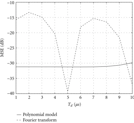
Figure 6 shows the estimation error under different de-lay profiles with Doppler frequency of 40 Hz. Figure 6a shows the estimation error with TU delay profile and 2-ray delay profile of Td = 5 microseconds, which is the
max-imal delay spread of TU while Figure 6b shows the esti-mation error with HT delay profile and 2-ray delay pro-file of Td = 17.2 microseconds which is the maximal
de-lay spread of HT. We also compared the results using the Fourier-transform-based method of [6]. We can see that for TU or HT, the proposed algorithm performs much better than the Fourier-transform-based method. However, for 2-ray channel with Td = 5 microseconds, the
Fourier-transform-based method performs the best. The reason is that Td = 5 microseconds is an integer multiplication of
the sampling period of the OFDM system, which is ts =
1/800 KHz = 1.25 microseconds. The impulse response of this 2-ray channel has energy only at the sampling instance
1 2 3 4 5 6 7 8 9 10
Td(µs)
−40
−35
−30
−25
−20
−15
−10
MSE
(dB)
Polynomial model Fourier transform
Figure7: Estimation error versus delay spread (SNR=20 dB, fD= 40 Hz, 2-ray,M×N=3×3,I×K=5×15).
0 25 50 75 100 125 150 Iterationk
5 8 11 14 17 20
W
indo
w
dimension
Time domain windowK
Frequency domain windowI
Adaptive Optimal
(a)
0 25 50 75 100 125 150
Iterationk 10
12 14 16 18 20
W
indo
w
dimension
Time domain windowK
Frequency domain windowI
Adaptive Optimal
(b)
0 25 50 75 100 125 150
Iterationk
−27
−26
−25
−24
−23
−22
−21
−20
−19
MSE
(dB)
Adaptive Optimal
(c)
0 25 50 75 100 125 150
Iterationk
−27
−26
−25
−24
−23
−22
−21
−20
−19
MSE
(dB)
Adaptive Optimal
(d)
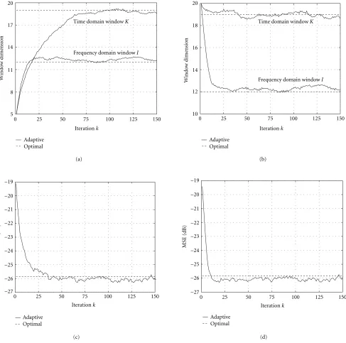
Figure8: Window dimensions adaptation (TU, SNR=10 dB, fD =40 Hz) (a) Window dimensions (starting from 5×5), (b) Window dimensions (starting from 20×20), (c) Estimation error (starting from 5×5), and (d) Estimation error (starting from 20×20).
using Fourier-transform-based on the sampling frequency of the OFDM system. The leakage greatly degrades the per-formance of the Fourier-transform-based method. In con-trast, the polynomial-model-based method performs consis-tently for the channels with same maximal delay spread and hence is more robust to the channel statistics. This is because the model errors are bounded by the same bound for the channels with the sameTd and fD as stated in Section 3.2.
Therefore, the performance of the polynomial-model-based channel estimation is not sensitive to the specific correlation
functions of the channels with the same Doppler frequency and maximum delay spread.
it performs consistently and outperforms the Fourier-transform-based method most of the time.
Figure 8 shows the window dimension adaptation. The window dimension variation is shown in Figures 8a and 8b. The estimation error is shown in Figures 8c and 8d. Two cases with different initial conditions are simulated, which are shown in Figures 8a and 8c and Figures 8b and 8d, re-spectively. In Figures 8a and 8c, the window dimension is 5 ×5 at the beginning, while in Figures 8b and 8d, it is 20×20. In both cases, after about 100 iterations, the algo-rithm converges to a window dimension of 12×10 and an estimation error under −26 dB. However, as mentioned in Section 6, smaller window dimensions are preferred for the sake of the computation complexity. With this adaptation algorithm, the polynomial-model-based method is not only robust to the specific correlation of the channel variation and dispersion, but also robust toTd and fD and can follow the
variation of the statistics of the channel. Moreover, in the previous simulation, fixed window dimensions are used, by applying this window dimension adaptation algorithm, the performance in Figure 6 can be further improved.
8. CONCLUSIONS
In this work, we proposed a channel estimation algorithm for the OFDM system with fading multipath channels, which is suitable for the applications in 3G wireless communications. The algorithm is based on the time-frequency polynomial model that exploits the correlation of the channel responses in both time and frequency domains. The channel response is approximated by a small number of time-frequency poly-nomial basis functions and estimated by first estimating the coefficients of the bases. The residual noise is significantly re-duced in this way, compared to the results when approxima-tion is only done either in time or frequency domain, and the estimator design is more flexible. Therefore, the approach is more robust to the channel statistics and system parameters than the existing Fourier-transform-based method. It does not require the delay profiles to be integer multiples of the system sampling period. Moreover, the algorithm can be im-plemented recursively and can adjust the model parameters adaptively to the delay and fading characteristics.
REFERENCES
[1] J. A. C. Bingham, “Multicarrier modulation for data trans-mission: An idea whose time has come,” IEEE Communica-tions Magazine, vol. 28, no. 5, pp. 5–14, 1990.
[2] L. J. Cimini Jr., “Analysis and simulation of a digital mo-bile channel using orthogonal frequency division multiplex-ing,”IEEE Trans. Communications, vol. 33, no. 7, pp. 665–675, 1985.
[3] P. S. Chow, J. M. Cioffi, and J. A. C. Bingham, “A practical dis-crete multitone transceiver loading algorithm for data trans-mission over spectrally shaped channels,” IEEE Trans. Com-munications, vol. 43, no. 2, pp. 773–775, 1995.
[4] J.-J. van de Beek, O. Edfors, M. Sandell, S. K. Wilson, and P. O. Ba¨orjesson, “OFDM channel estimation by singular value
de-composition,”IEEE Trans. Communications, vol. 46, no. 7, pp. 931–939, 1998.
[5] V. Mignone and A. Morello, “CD3-OFDM: a novel de-modulation scheme for fixed and mobile receivers,” IEEE Trans. Communications, vol. 44, no. 9, pp. 1141–1151, 1996. [6] Y. (G.) Li, L. J. Cimini Jr., and N. R. Sollenberger, “Robust
channel estimation for OFDM systems with rapid dispersive fading channels,”IEEE Trans. Communications, vol. 46, no. 7, pp. 902–915, 1998.
[7] E. W. Cheney, Introduction to Approximation Theory, McGraw-Hill, New York, NY, USA, 1966.
[8] H. N. Mhaskar,Introduction to the Theory of Weighted Polyno-mial Approximation, World Scientific Publishing, Singapore, 1996.
[9] D. K. Borah and B. D. Hart, “A robust receiver structure for time-varying, frequency-flat Rayleigh fading channels,”IEEE Trans. Communications, vol. 47, no. 3, pp. 360–364, 1999. [10] D. K. Borah and B. D. Hart, “Frequency-selective fading
channel estimation with a polynomial time-varying channel model,”IEEE Trans. Communications, vol. 47, no. 6, pp. 862– 873, 1999.
[11] M. Luise, R. Reggiannini, and G. M. Vietta, “Blind equal-ization/detection for OFDM signals over frequency-selective channels,”IEEE Journal on Selected Areas in Communications, vol. 16, no. 8, pp. 1568–1578, 1998.
[12] W. C. Jakes, Microwave Mobile Communications, Wiley, New York, NY, USA, 1974.
[13] Y. (G.) Li, N. Seshadri, and S. Ariyavisitakul, “Channel esti-mation for OFDM systems with transmitter diversity in mo-bile wireless channels,”IEEE Journal on Selected Areas in Com-munications, vol. 17, no. 3, pp. 461–471, 1999.
[14] P. A. Bello, “Characterization of randomly time-variant linear channels,” IEEE Trans. Communications Systems, vol. 11, no. 4, pp. 360–393, 1963.
[15] X. Wang and K. J. R. Liu, “OFDM channel estimation based on time-frequency polynomial model of fading multipath channel,” inVTC, Fall 2001.
[16] S. Haykin, Adaptive Filter Theory, Prentice Hall, Englewood Cliffs, NJ, USA, 1996.
Xiaowen Wang received her B.S. degree
from the Department of Electronics En-gineering, Tsinghua University, Beijing, China in 1993, and the M.S. and Ph.D. degrees from the Department of Electri-cal and Computer Engineering, University of Maryland, College Park, Md, in 1999 and 2000, respectively. From 1993 to 1996, Dr. Wang was a Teaching Assistant with Tsinghua University, Beijing, China. From
K. J. Ray Liureceived his B.S. degree from the National Taiwan University, and the Ph.D. degree from UCLA, both in electri-cal engineering. He is Professor of Electri-cal and Computer Engineering Department of University of Maryland, College Park. His research interests span broad aspects of signal processing architectures; multimedia signal processing, wireless communications and networking, information security, and