Distributed Optimization in Power Networks and General Multi-agent
Systems
Thesis by
Na Li
In Partial Fulfillment of the Requirements for the Degree of
Doctor of Philosophy
California Institute of Technology Pasadena, California
2013
c 2013
Acknowledgements
I am deeply grateful to my advisor Professor John Doyle and co-advisor Professor Steven Low for the con-tinuous support for my PhD study and research. Since September 2007, they have deeply influenced me in different aspects of my life, not only through their great guidance in research, but also through their patience, enthusiasm, encouragement, and genuine concern for students. John introduced me to a variety of areas, pro-vided the vision, and gave me the freedom and support to pursue various projects. He has very broad interests and is expert at extracting essentials almost for any topic. His passion, enthusiasm, and belief in science and research have been a great source of inspiration and motivation to me. Steven taught me how to integrate theory and practice in order to make contributions to real systems. He never scarifies practical applications for theoretical beauty, or vice versa. His high standards for the quality of work has encouraged me to pursue the perfection of the work. John and Steven, thanks for being such good role models for my academic career. I could not have imagined having better advisors for my graduate study.
My sincere gratitude goes to my former college research advisor, Professor Jeff Shamma. The research experience at Jeff’s lab in 2006 and 2007 introduced a new area, control and systems, to that little college girl and shape her later career path. Jeff has been helpful in providing advice many times during my graduate study and there were always so much for me to learn from any conversation we had. He was and remains one of my best role models for a scientist, mentor, and teacher.
the smart grid and for providing the great vision. Your insights, especially physical insights, always lead to great problems and solutions. Without you, I could not have done a coherent work for power grids. Jason, our collaboration dates back to my senior year in college. I was lucky to join Caltech as a PhD student at same time as you joined Caltech as a postdoc. Thank you for introducing me to the area of game theory and for teaching me the joy of “playing games” in academia and life. Lijun and Jason, I remember and will alway remember how you guide my work and revise my paper step by step. You were and will be my dear mentors and friends forever.
I also would like to thank other professors who has helped me grow up in the past years. Professor Adam Weirman, thank you for always making time to provide me advice and give me feedback about my work. You have set a great model for me to learn as a junior faculty. Professor Richard Murray, thank you for being on my PhD defense committee and for being available every time when I need help and advice.
I am grateful to my intelligent colleagues in Control & Dynamical Systems (CDS) and RSRG. Special gratitude goes to some current and past group members for fruitful collaborations and intriguing discussions. I wish to acknowledge an incomplete list of group members: Andrea Censi, Chenghao Chien, Jerry Cruz, Masoud Farivar, Lingwen Gan, Dennice Gayme, Shuo Han, Vanessa Jonsson, Andy Lamperski, Javad Lavaei, Minghong Lin, Zhenhua Liu, Nikolai Matni, Somayeh Sojoudi, Changhong Zhao, etc.
Furthermore, I would like to thank all those who helped me, including my friends and teachers; without them I would not be where I am today. Special thanks go to my friends at Caltech: Qi An, Ting Chen, Mingyuan Huang, Rui Huang, Yu Huang, Guanglei Li, Piya Pal, Rangoli Sharan, Zhiying Wang, Mao Wei, Xi Zhang, Guoan Zheng, Hongchao Zhou, Zicong Zhou, Zhaoyan Zhu, etc.
Abstract
The dissertation studies the general area of complex networked systems that consist of interconnected and active heterogeneous components and usually operate in uncertain environments and with incomplete infor-mation. Problems associated with those systems are typically large-scale and computationally intractable, yet they are also very well-structured and have features that can be exploited by appropriate modeling and computational methods. The goal of this thesis is to develop foundational theories and tools to exploit those structures that can lead to computationally-efficient and distributed solutions, and apply them to improve systems operations and architecture.
Specifically, the thesis focuses on two concrete areas. The first one is to design distributed rules to man-age distributed energy resources in the power network. The power network is undergoing a fundamental transformation. The future smart grid, especially on the distribution system, will be a large-scale network of distributed energy resources (DERs), each introducing random and rapid fluctuations in power supply, demand, voltage and frequency. These DERs provide a tremendous opportunity for sustainability, efficiency, and power reliability. However, there are daunting technical challenges in managing these DERs and opti-mizing their operation. The focus of this dissertation is to develop scalable, distributed, and real-time control and optimization to achieve system-wide efficiency, reliability, and robustness for the future power grid. In particular, we will present how to explore the power network structure to design efficient and distributed market and algorithms for the energy management. We will also show how to connect the algorithms with physical dynamics and existing control mechanisms for real-time control in power networks.
Contents
Acknowledgements iv
Abstract vi
1 Introduction 1
1.1 The smart power network . . . 1
1.1.1 Demand response: market models with appliance characteristics and the power net-work structure. . . 2
1.1.2 Optimal power flow (OPF): convexification and distributed power optimization . . . 3
1.1.3 Real-time energy balancing: economic automatic generation control (AGC) . . . 3
1.2 Decentralized optimization: a game theoretical approach . . . 4
1.3 Structure and contributions of the thesis . . . 6
I
Distributed Energy Management in Power Systems
8
2 Demand Response Using Utility Maximization 9 2.1 Introduction . . . 92.1.1 Summary . . . 11
2.1.2 Previous work . . . 12
2.2 System model . . . 13
2.2.1 Load sevice entity . . . 13
2.2.3 Energy storage . . . 14
2.3 Equilibrium and distributed algorithm . . . 15
2.3.1 Equilibrium . . . 15
2.3.2 Distributed algorithm . . . 18
2.4 Detailed appliance models . . . 19
2.4.1 Type 1 . . . 19
2.4.2 Type 2 . . . 21
2.4.3 Type 3 . . . 22
2.4.4 Type 4 . . . 22
2.5 Numerical Experiments . . . 23
2.5.1 Simulation setup . . . 23
2.5.2 Real-time pricing demand response . . . 26
2.5.3 Comparisons among different demand response schemes . . . 28
2.5.4 Battery with different cost . . . 30
2.5.5 Performance scaling with different numbers of households . . . 31
2.6 Conclusion . . . 31
3 Optimal Power Flow 33 3.1 Introduction . . . 33
3.2 Problem formulation . . . 35
3.2.1 Branch flow model for radial networks . . . 35
3.2.2 Optimal power flow . . . 36
3.3 Exact relaxation . . . 37
3.3.1 Second-order cone relaxation . . . 37
3.3.2 Sufficient condition for exact relaxation . . . 38
3.3.2.1 Line networks . . . 38
3.3.2.2 General radial networks . . . 44
3.4.1 Verifying sufficient conditions . . . 48
3.4.2 Simulation . . . 49
3.5 Conclusion . . . 49
4 Distributed Load Management Over the Power Network 50 4.1 Introduction . . . 50
4.2 Problem formulation & preliminary . . . 52
4.2.1 Problem formulation . . . 52
4.2.2 A decentralized optimization algorithm: predictor corrector proximal multiplier (PCPM) 54 4.2.3 Convexification of problem OPF . . . 55
4.3 Demand management through the LSE . . . 56
4.3.1 Distributed algorithm . . . 58
4.4 A fully decentralized algorithm . . . 59
4.5 Generalization to demand response over multiple time instants . . . 63
4.6 Case study . . . 65
4.6.1 Load management with an LSE . . . 66
4.6.2 Fully decentralized load management . . . 67
4.7 Conclusion . . . 68
5 Economic Automatic Generation Control 69 5.1 Introduction . . . 69
5.2 System model . . . 71
5.2.1 Dynamic network model with AGC . . . 71
5.2.2 Optimal generation control . . . 73
5.3 Reverse engineering of ACE-based AGC . . . 74
5.4 Economic AGC by forward engineering . . . 78
5.5 Case study . . . 81
5.7 Appendix: A partial primal-dual gradient algorithm . . . 83
II
Designing Games for Distributed Optimization
87
6 Optimization Problem with Coupled Objective Function 88 6.1 Introduction . . . 896.2 Problem setup and preliminaries . . . 92
6.2.1 An illustrative example . . . 93
6.2.1.1 Gradient methods . . . 93
6.2.1.2 A game theoretic approach . . . 94
6.2.2 Preliminaries: potential games . . . 94
6.2.3 Preliminaries: state based potential games . . . 95
6.3 State based game design . . . 98
6.3.1 A state based game design for distributed optimization . . . 98
6.3.2 Analytical properties of the designed game . . . 100
6.4 Gradient play . . . 102
6.4.1 Gradient play for state based potential games . . . 102
6.4.2 Gradient play for our designed game . . . 105
6.5 Illustrations . . . 106
6.5.1 A simple example . . . 106
6.5.2 Distributed routing problem . . . 107
6.6 Conclusion . . . 110
6.7 Appendix . . . 111
6.7.1 An impossibility result for game design . . . 111
6.7.2 Proof of Theorem 6.3 . . . 113
6.7.3 A Lemma for gradient play . . . 119
7 Optimization Problem with Coupled Constraints 122
7.1 Introduction . . . 122
7.2 Problem formulation . . . 124
7.3 A methodology for objective function design . . . 125
7.3.1 Design using exterior penalty functions . . . 125
7.3.2 Design using barrier functions . . . 130
7.4 An illustrative example . . . 132
7.5 Conclusion . . . 133
8 Distributed Optimization with a Time Varying Communication Graph 135 8.1 Introduction . . . 135
8.2 Preliminaries . . . 136
8.2.1 Problem setup . . . 136
8.3 State based game design . . . 138
8.3.1 A state based game design . . . 138
8.3.2 Analytical properties of the designed game . . . 140
8.4 Gradient play . . . 145
8.5 Illustrations . . . 147
8.6 Conclusion . . . 148
List of Figures
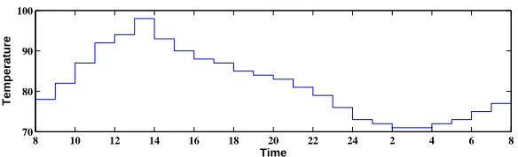
2.1 Outside Temperature over a day. . . 24
2.2 Total electricity demand under the real-time pricing demand response scheme without battery. 26 2.3 Electricity demand response for two typical households of different types without battery. The left panel shows the electric energy allocation for the household of the first type. The right panel shows the electric energy allocation for the household of the second type. . . 26
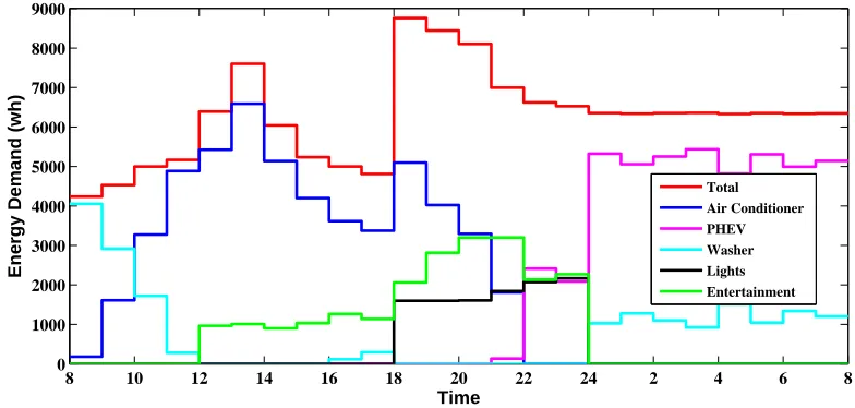
2.4 Total electricity demand under the real-time pricing demand response scheme with battery. . . 27
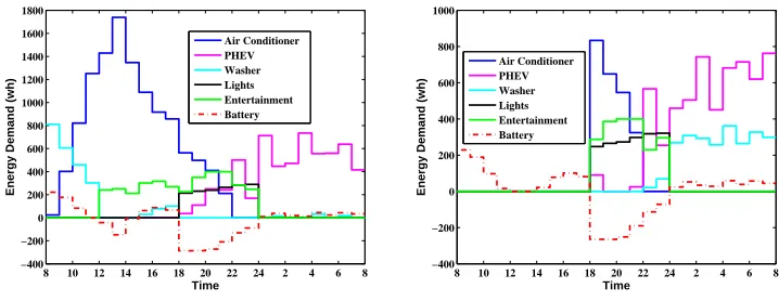
2.5 Electricity demand response for two typical households of different types with battery. The left panel shows the electric energy allocation for the household of the first type. The right panel shows the electric energy allocation for the household of the second type. . . 27
2.6 Room Temperature for two households of different types: the left panel shows the room tem-perature for the households with real-time pricing demand response without battery; the right panel shows the room temperature for the hoseholds with real-time pricing demand response with battery. . . 28
2.7 Electricity demand response under different schemes. . . 29
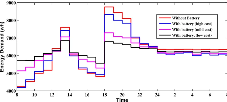
2.8 Electricity demand response with battery at different costs. . . 30
2.9 Electricity demand response without battery for different power networks with different num-bers of customers. . . 32
3.1 A one-line distribution network. . . 38
3.2 Schematic diagram of a 47-bus SCE distribution systems. . . 46
4.1 Dynamics of the distributed demand response algorithm: Busi’s calculatedpˆi. . . 66
4.2 Dynamics of the distributed demand response algorithm: LSE’s calculatedpifor each busi. . 67
4.3 Dynamics of the distributed demand response algorithm: Busi’s decisionpˆi. . . 67
5.1 A4-area interconnected system. . . 81
5.2 The ACE-based AGC. . . 82
5.3 The economic AGC. . . 82
5.4 The generation cost. . . 82
6.1 Simulation results for the optimization problem in (6.2.1). The top figure shows the evolution of the system costφ(v)using (i) centralized gradient algorithm, (ii) our proposed state based game design with gradient play, homogeneous step sizes, and synchronous updates (blue), and (iii) our proposed state based game design with gradient play, heterogeneous step sizes, and asynchronously updates (black). The bottom figure shows the evolution of agent1’s estimation errors, i.e.,e1 1−v1,e21−v2, ande31−v3, during the gradient play algorithm with homogeneous step sizes and synchronous updates. . . 108
6.2 Distributed Traffic Routing. . . 109
7.1 Simulation results for the economic dispatch problem. Subfigure 7.1(a) shows the simulation results when using gradient play applied to the state based game with exterior penalty functions using a tradeoff parameterµ= 60. The simulation demonstrates that the profile of generation levels quickly approaches (1.97,1.97,3.93,3.93)which is close to optimal. However, the generation levels do necessarily satisfy the demand. Subfigure 7.1(b) shows the simulation results when using gradient play applied to the state based game with barrier functions using a tradeoff parameter µ = 0.2. The simulation demonstrates that the profile of generation levels quickly approaches(2.03,2.03,4.02,4.02)which is close to optimal. Furthermore, the generation levels always exceed the demand in this setting. . . 134
8.1 Simulation results: The top figure shows the evolution of the system cost using the true gradi-ent descgradi-ent algorithm (red) and our proposed algorithm (black). The middle figure shows the evolution of the state based potential functionΦ(x(t),0). The bottom figure shows the evolu-tion of agenti’s estimation error as to agent1’s true value, i.e., e1
i −v1. Note that the error
List of Tables
2.1 Demand response without Battery. . . 30 2.2 Demand response with Battery. . . 31
3.1 Notations. . . 35 3.2 Line impedances, peak spot load KVA, Capacitors and PV generation’s nameplate ratings for
the distribution circuit in Figure 3.2. . . 47 3.3 Line impedances, peak spot load kVA, capacitors and PV generation’s nameplate ratings for
the distribution circuit in Figure 3.3. . . 47
Chapter 1
Introduction
The dissertation focuses on the general area of complex networked systems that consist of interconnected and active heterogeneous components that usually operate in uncertain environments and with incomplete in-formation. Problems associated with those systems are typically large-scale and computationally intractable, yet they are also very well-structured and have features that can be exploited by appropriate modeling and computational methods. The goal of this thesis is to develop foundational theories and tools to exploit those structures that can lead to computationally-efficient and distributed solutions, and apply them to improve systems operations and architecture.
Specifically, this dissertation focuses on two concrete areas. The first one is to design distributed rules to manage distributed energy resources in the power network; the second one is to design distributed optimiza-tion rules for more general multi-agent systems.
1.1
The smart power network
developing foundational theories, innovative algorithms, and novel architecture for scalable, distributed, real-time control and optimization. In this doctorate dissertation, I will present my work in pursuit of this direction through the following aspects:
1.1.1
Demand response: market models with appliance characteristics and the power
network structure.
Demand response is increasingly needed to improve power system efficiency and integrate renewable gener-ation. It will not only be applied to reduce peaks and shift load for economic benefits, but will increasingly be evoked to improve stability and reduce operating reserves by adapting elastic loads to intermittent and fluctuating renewable generation. Demand response involves both economic and engineering aspects of the power system, and requires coordinating actions among users and electric appliances while ensuring security, stability, and reliability of the grid.
We first study an abstract market model where a set of households are served by a single load-serving entity (LSE). The LSE may represent a regulated monopoly like most utility companies in the United States today, or a non-profit cooperative that serves a community of end users. We consider households that operate different appliances including air conditioners, washers, lighting, electric vehicles, batteries, etc, each of which provides a certain benefit depending on the pattern or volume of power it consumes. Each household wishes to optimally schedule its power consumption so as to maximize its individual net benefit subject to various consumption constraints. Based on utility maximization, we proposed a dynamic pricing scheme and a distributed approach for the LSE to coordinate users’ demand response to benefit the overall system, including reducing the peak load, smoothing the entire demand profile, and saving significant generation costs. This work serves as a good starting point to study the market dynamics and the residential model for demand response.
constraints. The OPF problem is general non-convex. This necessitates our work on OPF and its distributed solutions.
1.1.2
Optimal power flow (OPF): convexification and distributed power
optimiza-tion
The optimal power flow (OPF) problem is a fundamental problem that underlies many power systems op-erations and planning. It seeks to optimize a certain objective subject to the power flow constraints and the operation constraints. The OPF problem is, in general, non-convex and difficult to solve. Recently, convex optimization tools have been used to relax the OPF problem to a convex problem in order to explore the power network structure for better system operations. Previous work showed that convex relaxation is exact for the radial networks if there are no lower bounds on the power injection. However, this condition does not hold for various applications including demand response and Volt/VAR control. Thus we explore other sufficient conditions without removing the lower bounds on power injection. We provide a series of sufficient conditions to guarantee the exact relaxation of the OPF problem for the radial network when the voltage upper bound is removed or modified by an approximation. These conditions are verified to hold for a wide class of distribution circuits, and the resulting voltage is in the safe operation range.
Convexity does not only facilitate the design of effective pricing schemes for the power market involved in demand response, but also enables the development of tractable, scalable, and distributed algorithms for system operations. We design a locational marginal pricing scheme and distributed algorithms for the utility company to guide users’ decisions over a distribution network. Case studies on South California Edison distribution circuits showed that the algorithm converges to the optimum very fast. We further develop a fully decentralized OPF algorithm where the users make their own local decisions based only on local information and local communication with their direct neighbors.
1.1.3
Real-time energy balancing: economic automatic generation control (AGC)
be instantaneously updated to arbitrary values, which is not usually the case for power systems. Hence these algorithms cannot be implemented as real-time controls that are required or desired, as amplified by mitigat-ing fluctuations in renewable generation. For real-time control, the algorithm (derived from the optimization model) that governs the update of a physical variable must coincide with the real physical dynamics or the built-in control mechanisms that govern the evolution of that variable, namely that the computation is im-plicitly carried out by the real physical dynamics of the power network. This would also make local sensing sufficient for distributed control, e.g., distributed load management based on local frequency measurement. However, it imposes hard constraints on algorithm design as those conventional optimization algorithms such as the gradient algorithms are usually not consistent with the physical dynamics.
One way to take into account the impact of a built-in mechanism is to reverse-engineer this mechanism to find out what optimization problem it implicitly solves, and then incorporate the corresponding objective function into the optimization model for the design or control problem. As an initial step, we have studied automatic generation control (AGC). AGC uses deviations in generator speeds and/or frequency as control signals to invoke appropriate valve action in order to regulate the mechanical power generation in response to load changes. The main objective of AGC is to maintain power balance and nominal system frequency; however how to optimize AGC to improve energy efficiency is less studied. We reverse-engineered AGC by showing that the AGC can be formulated as a partial primal-dual gradient algorithm to solve an optimization problem. We extended the resulting optimization problem to include generation cost, and proposed a dis-tributed management scheme that is based only on local measurements and communications and takes into account the impact of AGC. This work provides a good starting point for developing a framework for sys-tematic design of distributed, low-complexity load/generation control mechanisms to achieve system-wide efficiency and robustness.
1.2
Decentralized optimization: a game theoretical approach
laws provide the groundwork for a decision making architecture that possesses several desirable attributes including real-time adaptation and robustness to dynamic uncertainties. However, realizing these benefits requires addressing the underlying complexity associated with a potentially large number of interacting agents and the analytical difficulties of dealing with overlapping and partial information. Furthermore, the design of such control laws is further complicated by restrictions placed on the set of admissible controllers which limit informational and computational capabilities.
Game theory is beginning to emerge as a powerful tool for the design and control of multiagent systems. Utilizing game theory for this purpose requires two steps. The first step is to model the agents as self-interested decision makers in a game theoretic environment. This step involves defining a set of choices and a local objective function for each decision maker. The second step involves specifying a distributed learning algorithm that enables the agents to reach a desirable operating point, e.g., a Nash equilibrium of the designed game. One of the core advantages of game theory is that it provides a hierarchical decomposition between the decomposition of the systemic objective (game design) and the specific local decision rules (distributed learning algorithms). For example, if the game is designed as a potential game then there is an inherent robustness to decision making rules as a wide class of distributed learning algorithms can achieve convergence to a pure Nash equilibrium under a variety of informational dependencies.
1.3
Structure and contributions of the thesis
The contribution of each chapter is listed below. All of the chapters can be read separately according to the readers’ interests and backgrounds.
Part I: Distributed Energy Management in Power Networks (Chapters 2, 3, 4, 5)
Chapter 2 studies a demand response problem where a set of households are served by a single load-serving entity (LSE) and each household operates different appliances. Based on utility maximization, we proposed a dynamic pricing scheme and a distributed approach for the utility company to coordinate users’ demand response to benefit the overall system, including reducing the peak load, smoothing the entire demand profile, and saving significant generation costs.
Chapter 3 focuses on the optimal power flow (OPF) problem, which is generally non-convex. We advocate a second-order cone relaxation for OPF using the branch flow model and provide sufficient conditions under which the relaxation is exact. These conditions are demonstrated to hold for a wide class of practical power distribution systems.
Chapter 4 studies the distributed load management over a radial distribution network, by formulating it as an optimal power flow (OPF) problem. We propose two different distributed mechanisms to achieve the optimum. In the first one, there is a load-serving entity to set the price signals in order to coordinate the users’ demand response and in the second one the users coordinate their decisions through local communications with neighbors.
Chapter 5 studies the real-time control mechanisms to balance generation and load. We focus on modify-ing automatic generation control (AGC) to keep energy balanced and also to make energy allocation efficient at the same time.
Part II: Designing Games for Distributed Optimization (Chapters 6, 7,8)
Chapter 6 propose a game design for distributed optimization where the optimization problem has coupled objective function but decoupled constraints. We also provide a learning algorithm and prove its convergence to an equilibrium in the game that we propose to use.
particular exterior penalty methods and barrier function methods, into the design of the agents’ objective functions.
Part I
Distributed Energy Management in
Chapter 2
Demand Response Using Utility
Maximization
[] Demand side management will be a key component of the future smart grid that can help reduce peak load and adapt elastic demand to fluctuating generations. We study an abstract market model where a set of households are served by a single load-serving entity (LSE). Each household operates different appliances including air conditioners, washers, lighting, electric vehicles, batteries, etc, each of which provides a certain benefit depending on the pattern or volume of power it consumes. Based on utility maximization, we proposed a dynamic pricing scheme and a distributed approach for the LSE to coordinate users’ demand response to benefit the overall system, including reducing the peak load, smoothing the entire demand profile, and saving significant generation costs.
2.1
Introduction
days in summer. Second, the lack of ubiquitous two-way communication in the current infrastructure pre-vents the participation of a large number of diverse users with heterogeneous and time-varying consumption requirements. Both reasons favor a simple and static mechanism involving a few large users that is sufficient to deal with the occasional need for load control, but both reasons are changing.
Renewable sources can fluctuate rapidly and by large amounts. As their penetration continues to grow, the need for regulation services and operating reserves will increase, e.g., [11, 12]. This can be provided by additional peaker units, at a higher cost, or supplemented by real-time demand response [12–16]. We believe that demand response will not only be invoked to shave peaks and shift load for economic benefits, but will increasingly be called upon to improve security and reduce reserves by adapting elastic loads to intermittent and random renewable generation [17]. Indeed, the authors of [12, 18, 19] advocate the creation of a distribution/retail market to encourage greater load side participation as an alternative source for fast reserves. Such an application, however, will require a much faster and more dynamic demand response than practiced today. This will be enabled in the coming decades by the large-scale deployment of a sensing, control, and two-way communication infrastructure, including the flexible AC transmission systems, the GPS-synchronized phasor measurement units, and the advanced metering infrastructure, which is currently underway around the world [20].
2.1.1
Summary
Specifically, in this chapter we consider a demand response problem where a set of households are served by a single load-serving entity (LSE). The LSE may represent a regulated monopoly like most utility companies in the United States today, or a non-profit cooperative that serves a community of end users. Its purpose is (possibly regulated) to promote the overall system welfare. The LSE purchases electricity on the wholesale electricity markets (e.g., day-ahead, real-time balancing, and ancillary services) and sells it on the retail market to end users. It provides two important values: it aggregates loads so that the wholesale markets can operate efficiently, and it hides the complexity and uncertainty from the users, in terms of both power reliability and prices.
We will consider households that operate different appliances including PHEVs and batteries and pro-pose a demand response approach based on utility maximization. Each appliance provides a certain benefit depending on the pattern or volume of power it consumes. Each household wishes to optimally schedule its power consumption so as to maximize its individual net benefit subject to various consumption and power flow constraints. We show that there exist time-varying prices that can align individual optimality with social optimality, i.e., under such prices, when the households selfishly optimize their own benefits, they auto-matically also maximize the social welfare. The LSE can thus use dynamic pricing to coordinate demand responses to the benefit of the overall system. We propose a distributed algorithm for the LSE and the cus-tomers to jointly compute this optimal prices and demand schedules. We also present simulation results that illustrate several interesting properties of the proposed scheme, as follows:
1. Different appliances are coordinated indirectly by real-time pricing, so as to flatten the total demand over different time-periods as much as possible.
2. Compared with no demand response or flat-price schemes, real-time pricing is very effective in shaping the demand: it not only greatly reduces the peak load, but also the variation in demand.
3. The integration of the battery helps reap more benefit from demand response: it not only reduces the peak load but further flattens the entire load profile and reduces the demand variation.
cost without hurting customers’ utility; here again, the battery amplifies this benefit.
5. The cost of the battery (such as its lifetime in terms of charging/discharging cycles) is important: the benefit of demand response increases with lower battery cost.
6. As the number of the households increases, the benefit of our demand response increases but will eventually saturate.
2.1.2
Previous work
There exists a large literature on demand response, see, e.g., [9, 21–29]. We briefly discuss some papers that are directly relevant to our chapter. First there are papers on modeling specific appliances. For instance, [21] and [22] consider the electricity load control with thermal mass in buildings; [23] considers the coordination of charging PHEV with other electric appliances. Then, there are papers on the coordination among different appliances. [24] studies electricity usage for a typical household and proposes a method for customers to schedule their available distributed energy resources to maximize net benefits in a day-ahead market. [25] proposes a residential energy consumption scheduling framework which attempts to achieve a desired trade-off between minimizing the electricity payment and minimizing the waiting time for the operation of each appliance in household in presence of a real-time pricing tariff by doing price prediction based on prior knowledge. While in practice, for different appliances, the household may have a different objective rather than waiting time for the operation of the appliance.
Notations. We useqi,a(t)to denote the power demanded by customeri for applianceaat time t. Then,
qi,a := (qi,a(t),∀t)denotes the vector of power demands overt= 1, . . . , T;qi := (qi,a,∀a∈ Ai)denotes
the vector of power demands for all appliances in the collectionAiof customeri; andq:= (qi,∀i)denotes
the vector of power demands from all customers. Similar convention is used for other quantities such as battery charging schedulesri(t), ri, r.
2.2
System model
Consider a setN of households/customers that are served by a load service entity (LSE). The LSE partici-pates in wholesale markets (day-ahead, real-time balancing, ancillary services) to purchase electricity from generators and then sell it to theN customers in the retail market. Even though wholesale prices can fluctu-ate rapidly by large amounts, currently most utility companies hide this complexity and volatility from their customers and offer electricity at a flat rate (fixed unit price), perhaps in multiple tiers based on a customer’s consumption. Even though the wholesale prices are determined by (scheduled or real-time) demand and supply and by congestion in the transmission network (except for electricity provisioned through long-term bilateral contracts), the retail prices are set statically independent of the real-time load and congestion. Flat-rate pricing has the important advantage of being simple and predictable, but it does not encourage efficient use of electricity. In this chapter, we propose a way to use dynamic pricing in the retail market to coor-dinate the customers’ demand responses to the benefit of individual customers and the overall system. We now present our model, describe how the utility should set their prices dynamically, how a customer should respond, and the properties of the resulting operating point.
We consider a discrete-time model with a finite horizon that models a day. Each day is divided intoT
timeslots of equal duration, indexed byt∈ T :={1,2,· · ·, T}.
2.2.1
Load sevice entity
customers. The design of the retail prices needs to at least recover the running costs of the the LSE, including the payments it incurs in the various wholesale markets. It is an interesting subject that is beyond the scope of this chapter. For simplicity, we make the important assumption that this design can be summarized by a cost functionC(Q, t)that specifies the cost for the LSE to provideQamount of power to theN customers at timet. The modeling of cost function is an active research issue [27, 29, 30]. Here we assume that the cost functionC(Q, t)is convex increasing inQfor eacht. The LSE sets the prices(p(t), t∈ T)according to an algorithm described below.
2.2.2
Customers
Each customeri ∈ N operates a setAi of appliances such as air conditioner, refrigerator, plug-in hybrid
electric vehicle (PHEV), etc. For each appliancea∈ Aiof customeri, we denote byqi,a(t)its power draw
at timet∈ T, and byqi,athe vector(qi,a(t), t∈ T)of power draws over the whole day. An applianceais
characterized by two parameters:
• a utility functionUi,a(qi,a)that quantifies the utility useriobtains when it consumesqi,a(t)power at
each timet∈ T; and
• a set of linear inequalitiesAi,aq
i,a≤ηi,aon the vector powerqi,a.
In Section 2.4, we will describe in detail how we model various appliances through appropriate matricesAi,a
and vectorηi,a. Note that inelastic load, e.g., minimum refrigerator power, can be modeled byqi,a(t)≥qi,a,
which says the appliance aof customeri requires a minimum powerqi,a at all times t. This is a linear inequality constraint and part ofAi,aq
i,a≤ηi,a.
2.2.3
Energy storage
In addition to appliances, a customer i may also possess a battery which provides further flexibility for optimization of its consumption across time. We denote byBithe battery capacity, bybi(t)the energy level
of the battery at timet, and byri(t)the power (energy per period) charged to (whenri(t)≥0) or discharged
the dynamics of the battery energy level by
bi(t) = t
X
τ=1
ri(τ) +bi(0) . (2.1)
Battery usually has an upper bound on charge rate, denoted byrmax
i for customeri, and an upper bound on
discharge rate, denoted by−rmin
i for customeri. We thus have the following constraints onbi(t)andri(t):
0≤bi(t)≤Bi, rimin≤ri(t)≤rimax . (2.2)
When the battery is discharged, the discharged power is used by other electric appliances of customeri. It is reasonable to assume that the battery cannot discharge more power than the appliances need, i.e.,−ri(t)≤
P
a∈Aiqi,a(t). Moreover, in order to make sure that there is a certain amount of electric energy in the
battery at beginning of the next day, we impose a minimum on the energy level at the end of control horizon:
b(T)≥γiBi, whereγi∈(0,1].
The cost of operating the battery is modeled by a functionDi(ri)that depends on the vector of charged/discharged
powerri := (ri(t), t∈ T). This cost, for example, may correspond to the amortized purchase and
mainte-nance cost of the battery over its lifetime, which depends on how fast/much/often it is charged and discharged. The cost functionDiis assumed to be a convex function of the vectorri.
2.3
Equilibrium and distributed algorithm
2.3.1
Equilibrium
With the battery, at each timetthe total power demand of customeriis
Qi(t) :=
X
a∈Ai
qi,a(t) +ri(t) . (2.3)
utility minus the utility’s cost of providing the electricity demanded by all the customers. Hence the LSE aims to solve:
Utility’s objective (max welfare):
max
q,r
X
i
X
a∈Ai
Ui,a(qi,a)−Di(ri)
!
−X
t
C X
i
Qi(t)
!
(2.4)
s. t. Ai,aqi,a ≤ηi,a, ∀a, i (2.5)
0 ≤ Qi(t) ≤ Qmaxi , ∀t, i (2.6)
ri ∈ Ri, ∀i (2.7)
whereQi(t)is defined in (2.3), the inequality (2.5) models the various customer appliances (see Section
2.4 for details), the lower inequality of (2.6) says that customeri’s battery cannot provide more power than the total amount consumed by alli’s appliances, and the upper inequality of (2.6) imposes a bound on the total power drawn by customeri. The constraint (2.7) models the operation of customeri’s battery with the feasible setRidefined by: for allt, the vectorsri∈ Riif and only if
0 ≤ bi(t) ≤ Bi, bi(T)≥γiBi (2.8)
rmin
i ≤ ri(t) ≤ rimax (2.9)
wherebi(t)is defined in terms of(ri(τ), τ ≤t)in (2.1).
By assumption, the objective function is concave and the feasible set is convex, and hence an optimal point can in principle be computed centrally by the LSE. This, however, will require the LSE to know all the customer utility and cost functions and all the constraints, which is clearly impractical. The strategy is for the LSE to set pricesp:= (p(t), t ∈ T)in order to induce the customers to individually choose the right consumptions and charging schedules(qi, ri)in response, as follows.
Given the price p, we assume that each customeri chooses the power demand and battery charging schedule (qi, ri) := (qi,a(t), ri(t),∀t,∀a ∈ Ai) so as to maximize its net benefit, the total utility from
customerisolves:
Customeri’s objective (max own benefit):
max
optimal to the utility company, i.e., maximizes the welfare (2.4).
The following result follows from the welfare theorem. It implies that setting the price to be the marginal cost of power is optimal.
Theorem 2.1. There exists an equilibriump∗ and(q∗
i, ri∗,∀i). Moreover,p∗(t) = C0(
P
iQ∗i(t)) ≥0 for
each timet.
Proof. Write the LSE’s problem as
max
(2.9). Clearly, an optimal solution(q∗, r∗)exists. Moreover, there exist Lagrange multipliersp∗
i(t),∀i, t,
such that (taking derivative with respect toQi(t))
Since the right-hand side is independent ofi, the utility company can set the prices asp∗(t) :=p∗
i(t)≥0for
alli. One can check that the KKT condition for the utility’s problem are identical to the KKT conditions for the collection of customers’ problems. Since both the utility’s problem and all the customers’ problems are convex, the KKT conditions are both necessary and sufficient for optimality. This proves the theorem.
2.3.2
Distributed algorithm
Theorem 2.1 motivates a distributed algorithm where the LSE and the customers jointly compute an equilib-rium based on a gradient algorithm, where the LSE sets the prices to be the marginal costs of electricity and each customer solves its own maximization problem in response. The model is that at the beginning of each day, the utility company and (the automated control agents of) the customers iteratively compute the electric-ity pricesp(t), consumptionsqi(t), and charging schedulesri(t), for each periodtof the day, in advance.
These decisions are then carried out for that day. Atk-th iteration:
• The LSE collects forecasts of total demands(Qi(t), ∀t)from all customersiover a communication
network. It sets the prices to the marginal cost
pk(t) =C0 X i
Qki(t) !
(2.11)
and broadcasts(pk(t),∀t)to all customers over the communication network.
• Each customeriupdates its demandqk
i and charging schedulerik after receiving the updatedpk,
ac-cording to
whereγ >0is a constant stepsize, and[·]Sidenotes projection onto the setS
ispecified by constraints
Whenγis small enough, the above algorithm converges [31].
2.4
Detailed appliance models
In this section, we describe detailed models of electric appliances commonly found in a household. We separate these appliances into four types, each type characterized by a utility functionUi,a(qi,a)that models
how much customerivalues the consumption vectorqi,a, and a set of constraints on the consumption vector
qi,a. The description in this section elaborates on the utility functionsUi,a(qi,a)and the constraintAi,aqi,a≤
ηi,ain the optimization problems defined in Section 2.3.
2.4.1
Type 1
The first type includes appliances such as air conditioners and refrigerators which control the temperature of customeri’s environment.
We denote byAi,1the set of Type 1 appliances for customeri. For each appliancea∈ Ai,1,Ti,ain(t)and
Tout
i,a (t)denote the temperatures at timetinside and outside the place that the appliance is in charge of, and
Ti,adenotes the set of timeslots during which customeriactually cares about the temperature. For instance,
for air conditioners,Tin
i,a(t)is the temperature inside the house,Ti,aout(t)is the temperature outside the house,
andTi,ais the set of timeslots when the resident is at home.
Assume that, at each timet ∈ Ti,a, customeriattains a utilityUi,a(Ti,a) :=Ui,a(Ti,ain(t), T comf i,a )when
the temperature isTin
i,a(t). The utility function is parameterized by a constantT comf
i,a which represents the
most comfortable temperature for the customer. We assume thatUi,a(Ti,ain(t))is a continuously differentiable,
concave function ofTin i,a(t).
The inside temperature evolves according to the following linear dynamics:
Ti,ain(t) =Ti,ain(t−1) +α(Ti,aout(t)−Ti,ain(t−1)) +βqi,a(t) (2.13)
thermal efficiency of the system: β > 0 if applianceais a heater andβ < 0if it is a cooler. Here, we defineTin
i,a(0)as the temperatureTi,ain(T)from the previous day. This formulation models the fact that the
current temperature depends on the current power draw as well as the temperature in the previous timeslot. Thus the current power consumption has an effect on future temperatures [9, 21, 22]. For each customeriand each appliancea ∈ Ai,1, there is a range of temperature that customeritakes as comfortable, denoted by
[Ti,acomf,min, T
comf,max
i,a ]. Thus we have the following constraint
Ti,acomf,min ≤ Ti,ain(t) ≤ T
comf,max
i,a , ∀t∈ Ti,a . (2.14)
We now express the constraints and the argument to the utility functions in terms of the load vector
qi,a:= (qi,a(t),∀t). Using equation (2.13), we can writeTi,ain(t)in terms of(qi,a(τ), τ = 1, . . . , t):
i,arepresents the temperature at timetif the applianceadoesn’t exist. It is determined by outside temperature and not controlled
as2
Ui,a(qi,a) :=
X
t∈Ti,a
Ui,a Ti,at + t
X
τ=1
(1−α)t−τβqi,a(τ), Ti,acomf
!
(2.17)
which is a concave function of the vectorqi,asinceUi,a(Ti,ain(t), T comf
i,a )is concave inTi,ain(t).
In addition, there is a maximum powerqmax
i,a (t)that the appliance can bear at each time, thus we have
another constraint on theqi,a:
0≤qi,a(t)≤qi,amax(t), ∀t .
2.4.2
Type 2
The second category includes appliances such as PHEV, dish washer, and washing machine. For these appli-ances, a customer only cares about whether the task is completed before a certain time. This means that the cumulative power consumption by such an appliance must exceed a threshold by the deadline [23–25].
We denote Ai,2 as the set of Type 2 appliances. For each a ∈ Ai,2, Ti,a is the set of times that the
appliance can work. For instance, for PHEV,Ti,ais the set of times that the vehicle can be charged. For each
customerianda∈ Ai,2, we have the following constraints on the load vectorqi,a:
qmin
i,a (t) ≤ qi,a(t) ≤ qi,amax(t), ∀t∈ Ti,a,
qi,a(t) = 0, ∀t∈ T \Ti,a
¯
Qmin i,a ≤
P
t∈Ti,aqi,a(t) ≤ Q¯
max i,a
whereqmin
i,a (t)andqi,amax(t)are the minimum and maximum power load that the appliance can consume at
timet, andQ¯min
i,a andQ¯maxi,a are the minimum and maximum total power draw that the appliance requires. If
2We abuse notation to useU
we setqmin
i,a (t) =qi,amax(t) = 0fort∈ T \Ti,a, we can rewrite these constraints as
qmin
i,a (t)≤qi,a(t)≤qi,amax(t), ∀t∈ T
¯
Qmin i,a ≤
P
t∈Ti,aqi,a(t)≤
¯
Qmax i,a .
(2.18)
The overall utility that customer iobtains from a Type-2 applianceadepends on the total power con-sumption byaover the whole day. Hence the utility function in the form used in Section 2.3 is:Ui,a(qi,a) :=
Ui,a(Ptqi,a(t)). We assume that the utility function is a continuously differentiable, concave function of
P
tqi,a(t).
2.4.3
Type 3
The third category includes appliances such as lighting that must be on for a certain period of time. A customer cares about how much light they can get at each timet. We denote byAi,3 the set of Type-3
appliances and byTi,athe set of times that the appliance should work. For each customerianda∈ Ai,3, we
have the following constraints on the load vectorqi,a:
qmin
i,a (t)≤qi,a(t)≤qi,amax(t), ∀t∈ Ti,a. (2.19)
At each time t ∈ Ti,a, we assume that customeriattains a utilityUi,a(qi,a(t), t)from consuming power
qi,a(t)on appliancea. The overall utility is thenUi,a(qi,a) :=PtUi,a(qi,a(t), t). Again, we assumeUi,ais
a continuously differentiable, concave function.
2.4.4
Type 4
The fourth category includes appliances such as TV, video games, and computers that a customer uses for entertainment. For those appliances, the customer cares about two things: how much power they use at each time they want to use the appliance, and how much total power they consume over the entire day.
We denote byAi,4the set of Type-4 appliances and byTi,a the set of times that customerican use the
customerianda∈ Ai,4, we have the following constraints on the load vectorqi,a:
qmin
i,a (t)≤qi,a(t)≤qi,amax(t), ∀t∈ Ti,a
¯
Qmin i,a ≤
P
t∈Ti,aqi,a(t)≤
¯
Qmax i,a
(2.20)
whereqmin
i,a (t)andqi,amax(t)are the minimum and maximum power that the appliance can consume at each
timet; Q¯min
i,a andQ¯maxi,a are the minimum and maximum total power that the customer demands for the
appliance. For example, a customer may have a favorite TV program that he wants to watch everyday. With DVR, the customer can watch this program at any time. However the total power demand from TV should at least be able to cover the favorite program.
Assume that customeriattains a utilityUi,a(qi,a(t), t)from consuming powerqi,a(t)on appliancea∈
Ai,4at timet. The time dependent utility function models the fact that the resident would get different benefits
from consuming the same amount of power at different times. Take watching the favorite TV program as an example. Though the resident is able to watch it at any time, he may enjoy the program at different levels at different times.
2.5
Numerical Experiments
In this section, we provide numerical examples to complement the analysis in the previous sections.
2.5.1
Simulation setup
We consider a simple system with 8 households in one neighborhood that join in the demand response system. The households are divided into two types evenly. For the households of the first type (indexed by i = 1,2,3,4), there are residents staying at home for the whole day; for the households of the second type
(indexed byi= 5,6,7,8), there is no person staying at home during the day time (8am-6pm). A day starts at 8am, i.e.,t ∈ T corresponds to the hour[7 +t(mod24),8 +t(mod24)]. Each household is assumed to have 6 appliances: air conditioner, PHEV, washing machine, lighting, entertainment,3and electric battery.
8 10 12 14 16 18 20 22 24 2 4 6 8 70
80 90 100
Time
Temperature
Figure 2.1. Outside Temperature over a day.
The basic parameters of each appliance used in simulation are shown as follows.
1. Air conditioner: This appliance belongs to Type 1. The outside temperature is shown in Figure 2.1. It captures a typical summer day in Southern California. For each resident, we assume that the comfort-able temperature range is[70F,79F], and the most comfortable temperature is randomly chosen from [73F,77F]. The thermal parametersα= 0.9andβis chosen randomly from[−0.011,−0.008]. For each household’s air conditioner, we assume thatqmax = 4000whandqmin = 0wh, and the utility
function takes the form ofUi,a(Ti(t)) :=ci,a−bi,a(Ti,a(t)−Ti,acom)2, wherebi,aandci,aare positive
constants. We further assume that the residents will turn off the air conditioner when they go to sleep.4 The households of the first type care about the inside temperature through the whole day, and the other households care about the inside temperature during the timeTi,a={18,· · ·,24,1,· · · ,7}.
2. PHEV: This appliance belongs to Type 2. We assume that the available charging time,Ti,a ={18,· · · ,24,1,· · · ,7},
is the same for all houses. The storage capacity is chosen randomly from [5500wh,6000wh]; and the minimum total charging requirement is chosen randomly from[4800wh,5100wh]. The minimum and maximum charging rates are0w and2000w. The utility function takes the form ofUi,a(Q) =
bi,aQ+ci,a, wherebi,aandci,aare positive constants.
3. Washing machine: This appliance belongs to Type 2. For the households of the first type, the avail-able working time is the whole day; for the other households, the availavail-able working time is Ti,a =
{18,· · · ,24,1,· · · ,7}. The minimum and maximum total power demands are chosen from[1400wh,1600wh] and[2000wh,2500wh]respectively. The minimum and maximum working rate are0wand1500w
re-4Notice that the outside temperature during 23pm-8am in Southern California is comfortable. It is common that customers turn off
spectively. The utility function takes the form ofUi,a(Q) =Q+ci,a, whereci,ais a positive constant.
4. Lighting: This appliance belongs to Type 3. Ti,a = {18,· · ·,23}, and the minimum and maximum
working power requirements are200wand800wrespectively. The utility function takes the form of
Ui,a(qi,a(t)) =ci,a−(bi,a+qi,a¯q(t))−1.5, wherebi,aandci,aare positive constants.
5. Entertainment: This appliance belongs to Type 4. For the households of the first type,Ti,a={12,· · · ,23},
Qmax
i = 3500wh, andQmini = 1200wh; for the other households,Ti,a ={18,· · · ,24},Qmaxi =
2000wh, andQmin
i = 500wh. The minimum and maximum working rate are0wand400w
respec-tively. The utility function takes the form ofUi,a(qi,a(t)) =ci,a−(bi,a+qi,aq¯(t))−1.5, wherebi,aand
ci,aare positive constants.
6. Battery: The storage capacity is chosen randomly from[5500wh,6500wh]and the maximum charg-ing/discharging rates are both 1800w. We set γi = 0.5, and the cost function takes the following
form:
whereη1,η2, η3, δ andci,b are positive constants. The first term captures the damaging effect of
fast charging and discharging; the second term penalizes charging/discharging cycles;5the third term
captures the fact that deep discharge can damage the battery. We setδ= 0.2.6
On the supply side, we assume that the electricity cost function is a smooth piecewise quadratic function [32], i.e.,
2is smaller thanη1, the cost function is a positive convex function. The second item can also be seen as a correction term to the first term.
wherecm> cm−1> . . .≥c1>0.
2.5.2
Real-time pricing demand response
Let us first see the performance of our proposed demand response scheme with real-time pricing, without and with battery.
Figure 2.2. Total electricity demand under the real-time pricing demand response scheme without battery.
8 10 12 14 16 18 20 22 24 2 4 6 8
Figure 2.3. Electricity demand response for two typical households of different types without battery. The left panel shows the electric energy allocation for the household of the first type. The right panel shows the electric energy allocation for the household of the second type.
total power demand at different times as much as possible.
Figure 2.4. Total electricity demand under the real-time pricing demand response scheme with battery.
8 10 12 14 16 18 20 22 24 2 4 6 8
Figure 2.5. Electricity demand response for two typical households of different types with battery. The left panel shows the electric energy allocation for the household of the first type. The right panel shows the electric energy allocation for the household of the second type.
Figure 2.4 shows the total electricity demand under the real-time pricing demand response scheme with battery; Figure 2.5 shows the corresponding electricity allocation for two typical households of different types. Those figures show the value of the battery for demand response: it not only reduces the peak load but also helps to further flatten the total power demand at different times.
8 10 12 14 16 18 20 22 24 2 4 6 8
Figure 2.6. Room Temperature for two households of different types: the left panel shows the room temper-ature for the households with real-time pricing demand response without battery; the right panel shows the room temperature for the hoseholds with real-time pricing demand response with battery.
the comfortable temperature in both cases. The battery is able to keep the temperature closer to the most comfortable temperature.
2.5.3
Comparisons among different demand response schemes
In order to evaluate the performance of our proposed demand response scheme, we consider three other schemes. In the first scheme the customer is not responsive to any price or cost, but just wants to live a comfortable lifestyle; in the second and third ones, the customer responds to a certain flat price.
1. No demand response: The customers just allocate their energy usage according to their own prefer-ence without paying any attention to the price, i.e., they just optimize their utility without caring about their payment. For example, the customer sets the air conditioner to keep the temperature to the most comfortable level all the time; charges PHEV, washes clothes and watches TV at the favorite times. The electricity demand over a day under this scheme is shown by the blue plot in Figure 2.7.
2. Flat price scheme 1:In this scheme, the customer is charged a flat pricep, such that
p= (1 + ∆)
price. Eventually,pk will converge to a fixed point, which is the flat price we need.7 The electricity
demand over a day under this scheme is shown by the magenta plot in Figure 2.7.
3. Flat price scheme 2: In this scheme we use the information obtained from our proposed real-time pricing demand response scheme to set a flat pricep. We collect the price{p(t)}t∈T and total power demand{Q(t)}t∈T information under the real time pricing scheme and then set the flat price asp=
P
t∈Tp(t)Q(t) P
t∈TQ(t) . The electricity demand over a day under this scheme is shown by the black plot in
Figure 2.7.
8 10 12 14 16 18 20 22 24 2 4 6 8
0 0.5 1 1.5
2x 10 4
Time
Energy Demand (wh)
No demand response Flat price scheme 1 Flat Price scheme 2 Real−time price; no battery Real−time price; with battery
Figure 2.7. Electricity demand response under different schemes.
Figure 2.7 also shows the electricity demand response under the real-time pricing scheme with and with-out battery. We see that the real-time pricing demand response scheme is very effective in shaping the demand: not only is the peak load reduced greatly, but also the variation in power demand decreases greatly; with the integration of the battery, the peak load and the variation in power demand will be reduced further.
Table 2.1 summarizes the differences among the three pricing schemes. We see that the real-time pricing scheme can increase the load factor greatly and save a large amount of generation cost without hurting cus-tomers’ utility. The integration of the battery can further increase the load factor and reap larger savings in generation cost.
Table 2.1. Demand response without Battery.
Load Factor 0.3587 0.4495 0.4577 0.7146 0.8496
Peak Demand 18.8 kwh 14.7 kwh 13 kwh 8.76 kwh 7.29 kwh
Total Demand 162 kwh 158 kwh 153 kwh 150 kwh 148 kwh
Generation Cost
$64.41 $45.49 $41.80 $32.82 $31.50
Total Payment $137.40a $ 54.59 $58.56 $57.42 $55.69
Customers’ Utility
$212.41 $201.72 $200.14 $198.82 $198.82b
Customers’ Net Utilityc
$75.01 $147.14 $141.57 $141.40 $143.13
Social Welfare $148.00 $156.24 $158.33 $166.00 $167.32
aThe price at each time slot is set as the real-time marginal generation cost.
bWhen there is a battery, a customer’s utility is defined as the benefits the customer gets from electric appliances minus the battery
cost.
cCustomers’ net utility is defined as customers’ utility minus payment.
2.5.4
Battery with different cost
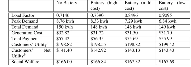
One of the challenges in the integration of the battery is its economic (in)viability because of high battery cost. In order to study the impact of battery cost on demand response, we consider three scenarios with high, mild, and low cost, by choosing different scaling factors (10, 1 and 0.1) for the battery cost in the objective function. Figure 2.8 shows the electricity demand under the real-time pricing scheme with batteries of different costs.
8 10 12 14 16 18 20 22 24 2 4 6 8
Figure 2.8. Electricity demand response with battery at different costs.
Table 2.2. Demand response with Battery. No Battery Battery
(high-cost)
Battery (mild-cost)
Battery (low-cost)
Load Factor 0.7146 0.7390 0.8496 0.9095
Peak Demand 8.76 kwh 8.33 kwh 7.29 kwh 6.84 kwh
Total Demand 150 kwh 148 kwh 148 kwh 149 kwh
Generation Cost $32.82 $31.72 $31.50 $31.70
Total Payment $57.42 $56.35 $55.69 $55.99
Customers’ Utilitya $198.82 $198.55 $198.82 $199.42
Customers’ Net Utilityb
$141.40 $142.92 $143.13 $143.43
Social Welfare $166.00 $166.84 $167.32 $167.69
aA customer’ utility is defined as the benefits the customer gets from electric appliances minus the battery cost. bA customer’ utility is defined as the customer’s utility minus the payment.
response.
2.5.5
Performance scaling with different numbers of households
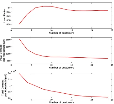
In order to study the effect of the system size on the performance of our demand response scheme, we simulate systems with the number of customers beingN = 2,4,6,· · ·,24. Figure 2.9 summarizes three interesting characteristic factors for the demand response systems with different numbers of households. We see that as the number of households increases, the load factor will first increase till a maximum value and then decrease a bit and finally level off, but the peak load and total demand at each household will decrease and finally level off. This shows that as the number of the households increases, our demand response scheme will reap more benefits but the gain will eventually saturate.
2.6
Conclusion
0 5 10 15 20 25 0.54
0.58 0.62 0.66 0.7
Number of customers
Load Factor
0 5 10 15 20 25
900 1200 1500 1800
Number of customers Peak Demand per Household (wh)
0 5 10 15 20 25
1.6 1.8 2 2.2 2.4x 10
4
Number of customers
Total Demand
per Household (wh)
Figure 2.9. Electricity demand response without battery for different power networks with different numbers of customers.
Chapter 3
Optimal Power Flow
[] In the previous chapter, we only consider demand response that balances aggregate load and supply, and abstract away the underlying power network. We will consider demand response in a radial distri-bution network in the next chapter by formulating it as an optimal power problem. In this chapter, we will focus on the optimal power flow problem, which is generally nonconvex. We advocate a second-order cone relaxation for OPF using the branch flow model and provide sufficient conditions under which the relaxation is exact. These conditions are demonstrated to hold for a wide class of practical power distribution systems.
3.1
Introduction
sufficient condition is derived in [44] under which the SDR is exact. This condition is shown to essentially hold in various IEEE test systems. While this line of research has generated a lot of interest, limitations of the SDR have also been studied in [45] using 3, 5, and 7-bus system. Moreover, if SDR fails to provide exact re-laxations, the solutions produced by the SDR are physically meaningless in those cases. Remarkably, it turns out that if the network is radial, then the sufficient condition of [44] always holds, provided that the bounds on the power flows satisfy a simple pattern [46–48]. This is important as almost all distribution systems are radial networks.
Indeed, for radial networks, different convex relaxations have also been studied using branch flow models. The model considered in this chapter is first proposed in [35, 36] for the optimal placement and sizing of switched capacitors in distribution circuits for Volt/VAR control. Recasting the model as a set of linear constraints together with a set of quadratic equality constraints, references [49] [33] propose a second-order-cone (SOC) convex relaxation, and prove that the relaxation is exact for radial networks, when there are no upper bounds on the loads. See also [50] for an SOC relaxation of a linear approximation of the branch flow model in [35, 36], and [51–53] for other branch flow models.
Ignoring upper bounds on the load may be unrealistic, e.g., in the context of demand response. In a previous paper [34], we prove that the SOC relaxation is exact for radial networks, provided there are no upper bounds on the voltage magnitudes and several other sufficient conditions hold. Those sufficient conditions however place strong requirements on the impedance of the distribution lines and on the load and generation patterns in the radial network. In this chapter, we propose less restrictive sufficient conditions under which the SOC relaxation is exact. As examples, we show that these conditions hold in two distribution circuits of the Southern California Edison (SCE), with high penetration of photovoltaic (PV) generation. Roughly speaking, these sufficient conditions hold in many real distribution systems wherev ∼1p.u.,p, q <1p.u. ,
r, x << 1p.u., and xr is bounded. Here,v, p, q are the bus voltage, real power consumption, and reactive power consumption, andr, xare the resistance and reactance of the distribution lines. Moreover, we provide upper bounds on the voltage magnitudes for the SOC relaxation solutions. This would facilitate the voltage regulation in distribution systems.
in Section 3.3 sufficient conditions under which the SOC relaxation is exact for radial networks when there are no upper bounds on bus voltage magnitudes. Finally, in Section 3.4, we illustrate these sufficient conditions using two real-world distribution circuits.
3.2
Problem formulation
3.2.1
Branch flow model for radial networks
Table 3.1. Notations.
Vi,vi complex voltage on busiwithvi=|Vi|2
si=pi+iqi complex net load on busi
Iij,`ij complex current from busesitojwith`ij =|Iij|2
Sij =Pij+iQij complex power flowing out from busesito busj
zij =rij+ixij impedance on line(i, j)
Consider a radial distribution circuit that consists of a set N of buses and a setE of distribution lines connecting these buses. We index the buses inNbyi= 0,1, . . . , n, and denote a line inEby the pair(i, j) of buses it connects. Bus0represents the substation and other buses inN represent branch buses. For each line(i, j)∈E, letIij be the complex current flowing from busesitoj,zij =rij+ixij the impedance on
line(i, j), andSij = Pij+iQij the complex power flowing from busesi to busj. On each busi ∈ N,
letVi be the complex voltage andsi be the complex net load, i.e., the consumption minus generation. As
customary, we assume that the complex voltageV0on the substation bus is given.
The branch flow model was first proposed in [35, 36] to model power flows in a steady state in a radial distribution circuit. We introduce here an abridged version of the branch flow model; see, e.g., [33, 34] for more details.
pj = Pij−rij`ij−
X
k:(j,k)∈E
Pjk, j= 1, . . . , n (3.1)
qj = Qij−xij`ij−
X
k:(j,k)∈E
Qjk, j= 1, . . . , n (3.2)
vj = vi−2(rijPij+xijQij) + (r2ij+x2ij)`ij,(i, j)∈E (3.3)
`ij =
P2
ij+Q2ij
vi
where`ij :=|Iij|2,vi :=|Vi|2, andpiandqiare the real and reactive net loads at nodei. Equations (3.1)–
(3.4) define a system of equations in the variables(P, Q, `, v) := (Pij, Qij, `ij,(i, j)∈E, vi, i= 1, . . . , n),
which do not include phase angles of voltages and currents. Given a(P, Q, `, v), these phase angles can be uniquely determined for radial networks. This is not the case for mesh networks; see [33] for exact conditions under which phase angles can be recovered for (an extension of the model here for) mesh networks.
3.2.2
Optimal power flow
Consider the problem of minimizing a cost function over the network where the optimization variables are
p:= (p1, . . . , pn),q:= (q1, . . . , qn), as well as(P, Q, `, v). Let
i andqci are the real and reactive power consumption at node i, andp g i andq
g
i are the real and
reactive power generation at nodei. In addition to power flow equations (3.1)–(3.4), we impose the following constraints on power consumption and generation:
pc
Here, equation (3.7) models additional constraints on(pc
i, qic)and(p g i, q
g
i). For example, for PV generators,
(pgi)2+ (q
Finally, the voltage magnitudes must be maintained above certain thresholds:
vi ≤ vi, i= 1, . . . , n. (3.8)
on theoptimalvoltage magnitudes.
The objective of the optimal power flow problem is to minimize the power generation costsCi(pgi), the
power lossesri,j`i,j, and maximize the user utilitiesfi(pci):1
OPF is NP hard in general, due to the quadratic equality constraint (3.4).
3.3
Exact relaxation
3.3.1
Second-order cone relaxation
Following [33, 34, 49], we relax the quadratic equalities in (3.4) into inequalities and consider the following convex relaxation of OPF.
Obviously, ROPF provides a lower bound on OPF. It was shown in [33, 49] that this relaxation is exact when there are no upper bounds on the real and reactive power consumptions in (3.5) but with upper bounds on the voltage magnitudes in (3.8).
1We can also include in the objective function of the costC
0
P
(0,j)∈EP0,j
The main result of this chapter is a variety of sufficient conditions for exact relaxation when there are no upper bounds on the voltage magnitudes. Given a solution of the relaxed problem ROPF, one can always check if equality is attained in (3.4). If it is, then the relaxed solution is optimal for the original problem OPF as well.