Direct Integration of Fourth Order Initial and Boundary Value Problems using Nyström Type Methods

Direct Integration of Fourth Order Initial and Boundary

Value Problems using Nyström Type Methods

S. N. Jator

_{, E. O. Adeyefa}

Abstract Nyström type methods are widely used for the numerical integration of initial value problems (IVPs) in ordinary dierential equations (ODEs). Specically, they are extensively used for directly solving second order IVPs. Nevertheless, they are not normally used for the numerical integration of boundary value problems (BVPs). This paper focuses on the formulation of a family of block Nyström type methods (BNM (η, p)) for the numerical solution of fourth order IVPs and BVPs, whereηis the number of o-grid points and p is the order of the method. The family of BNM (η, p) is formulated from contin-uous schemes obtained via collocation and interpola-tion techniques and applied in a block-by-block man-ner as numerical integrators for fourth order ODEs. The convergence properties of this family of methods are discussed via zero-stability and consistency. Nu-merical examples are included and comparisons are made with existing methods in the literature.

Keywords: Fourth Order Ordinary Dierential Equa-tions, Zero-stability and consistency, Block Nyström Method, Convergence

AMS Subject Classication: 65L05, 65L06

1 Introduction

The theory of dierential equations (DEs) has connec-tions with several elds such as engineering, science, and management. In particular, DEs have applications in uid dynamics (see Alomari et al. [3]), beam theory (see Jator [21]), electric circuits (see Boutayeb and Chetouani [8]), ship dynamics (see Wu et al. [35], Twizell [32], Cortell [11]) and neural networks (see Malek and Bei-dokhti [27]). They are also applied to the reaction and diusion of chemicals, the dynamics of populations in biology, the development and treatment of diseases in medicine, molecular dynamics, the motion of rocket, and several other areas. So, the demand for the solution of DEs is on the increase as the quest for numerical meth-ods has increasingly been of much interest to researchers owing to the fact that most of these DEs are dicult to solve or their analytical solutions do not exist. Thus, the

∗a _{Department of Mathematics and Statistics, Austin Peay}

State University, Clarksville, TN 37044 USA. b _{Department of}

Mathematics, Federal University Oye-Ekiti, Ekiti State, Nigeria. Corresponding author: [email protected]

focus of this paper is to develop a family of block Nys-tröm type methods for the numerical solution of the ODE of the form

yiv= f(x, y, y, y, y), x∈[x₀, xN], (1)

subject to initial conditions

y(x₀) =y₀, y(x₀) =y₀, y(x₀) =y₀, y(x₀) =y₀

which are not a restriction on the proposed method, since the method can also handle ODEs with Dirichlet, Neu-mann or Robin boundary conditions with only minor modications in the boundary conditions.

The IVP of the form (1) is solved by reduction to an equivalent system of rst order ODE and an appropriate numerical method is employed to solve the resultant sys-tem (see Adesanya et al. [1], Butcher [10], Lambert [25], Hairer et al. [17], and Dormand [13]). This approach has been reported to increase the number of equations four times and thereby more function evaluations need to be evaluated and hence resulting in a longer execution time and more computational eort (see Jator [21], Awoyemi ( [4],[6]), Waeleh et al. [34], Mehrkanoon [28]). Moreover, Bun and Vasil'yer [9] reported that the in some instances the system of equations to be solved when the method of reduction is applied cannot be solved explicitly with respect to the derivatives of the highest order.

A successful application of numerical algorithm for di-rectly solving a general fourth order initial value problems of the form (1) has been demonstrated in the literature (see Awoyemi ( [5],[6]), Kayode ([22], [23])). However, all these methods were implemented in predictor-corrector mode and hence, according to Jator, (Jator [21]) the im-plementation of such schemes is more costly since the subroutines for incorporating the starting values lead to lengthy computational time. Besides, they advance the numerical integration of the ordinary dierential equa-tions in one-step at a time, which leads to overlapping of the piecewise polynomials solution model. To address the setback of the predictor-corrector method, Vigo-Aguiar and Ramos [33], Jator [20], Mohammed [29], Kayode et al. [24], Awoyemi et al. [7], Yap and Ismail [36], Hussain et al. [19], Adeyefa [2] among others independently pro-posed block methods for solving higher order ordinary dierential equation which do not require the develop-ment of separate predictors, but simultaneously generate approximations at dierent grid points within the interval

IAENG International Journal of Applied Mathematics, 49:4, IJAM_49_4_33

of integration without overlapping of sub-intervals expe-rienced in the predictor-corrector method. Furthermore, the BNM (η, p)is superior to those mentioned above since

it is equipped with block extension for solving BVPs. The aim of developing new methods has always been to

improve on the eciency and convergence of existing methods with the ultimate aim of reducing the error of

approximation. Thus, in what immediately follows in Section 2, we formulate the proposed methods for directly integrating fourth order ODEs. The analysis of

the BNM (η, p)is discussed in Section 4, the

implementation of the methods is given in Section 5 and numerical examples are given to show the eciency of the methods in Section 6. Finally, the conclusion of the

paper is discussed in Section 7.

2 Development of the BNM

(

η, p

)

In order to numerically integrate (1), we consider the partition Q_N given by Q_N := {x_n = x₀ +nh}, n= 0,1, . . . , N,h=xN−x0

N ,

and then use the proposed BNM(η, p) consisting of the

following discrete formulas

yn+1=α0yn+hα₀yn +h2α0yn+h3α0yn

+h4

⎛ ⎝1

j=0

βjfn+j+ η

j=1

βcjfn+cj ⎞ ⎠

yn+ci=αi,0yn+hαi,0yn +h2αi,0yn+h3αi,0yn

+h4

⎛ ⎝1

j=0

βi,jfn+j+ η

j=1

βi,cjfn+cj ⎞ ⎠,

hy_n+1=α₁y_n+hα₁y_n+h2α₁y_n+h3α₁y_n

+h4

⎛ ⎝1

j=0

γjfn+j+ η

j=1

γcjfn+cj ⎞ ⎠

hy_n+ci =α_i,1y_n+hα_i,1y_n+h2α_i,1y_n+h3α_i,1y_n

+h4

⎛ ⎝1

j=0

γ_i,jf_n+j+

η

j=1

γ_i,cjf_n+cj

⎞ ⎠,

h2y_n+1=α₂y_n+hα₂y_n+h2α₂y_n+h3α₂y_n

+h4

⎛ ⎝1

j=0

δ_jf_n+j+

η

j=1

δ_cjf_n+cj

⎞ ⎠

h2y_n+ci =α_i,2y_n+hα_i,2y_n +h2α_i,2y_n+h3α_i,2y_n

+h4

⎛ ⎝1

j=0

δ_i,jf_n+j+

η

j=1

δ_i,cjf_n+cj

⎞ ⎠,

h3y_n+1=α₃y_n+hα₃y_n+h2α₃y_n+h3α₃y_n

+h4

⎛ ⎝1

j=0

κ_jf_n+j+

η

j=1

κ_cjf_n+cj

⎞ ⎠

h3y_n+ci =αi,3yn+hαi,3yn +h2αi,3yn+h3αi,3yn

+h4

⎛ ⎝1

j=0

κi,jfn+j+ η

j=1

κi,cjfn+cj ⎞ ⎠

where

yn+1, yn+ci, hyn+1, hyn+ci, h2yn+1, h2yn+ci,

h3y_n+1, h3y_n+cii= 1, . . . , η (2)

to integrate (1) over the partition considered, where

α_k, α_i,k, α_k, α_i,k, α_k, α_i,k, α_k, α_i,k, β_j, β_i,j, β_cj, β_i,cj, γ_j, γ_i,j, γ_cj, γ_i,cj, δ_j, δ_i,j, δ_cj, δ_i,cj, κ_j, κ_i,j, κ_cj, κ_i,cj, k= 1, . . . ,3are coecients andcjare the o-grid points.

The coecients of the methods are chosen so that the method integrates the ODE (1) exactly, where the solu-tions are members of the linear space1, x, . . . , xm+w−1_,

where m is the number of interpolation points and w is the number of collocation points. We note that

yn+j and yn+cj denote the numerical approximations to the analytical solutions y(x_n+j) and y(x_n+cj)

re-spectively; and f_n+j = f(x_n+j, y_n+j, y_n+j, y_n+j, y_n+j)

and f_n+cj = f(x_n+cj, y_n+cj, y_n+cj, y_n+cj, y_n+cj). The

coecients of (2) are provided by the continuous scheme derived next.

2.1 Continuous approximation for the BNM

In general, the coecients of (2) are chosen so that the method integrates the ODE (1) exactly, where the solutions are members of the linear space

U(x) = (U₀(x), U₁(x), ..., Um+w−1(x)), Uj(x) = xj, j =

0,1, . . . , m+w−1are basis functions. In order to obtain

the coecients in (2), we begin by seeking an approxi-mate solution of the form

Y(x) =

m+w−1

j=0

ajUj(x) =U(x)ΥT (3)

on the interval [xn, xn+1], where T is the transpose, Υ = (a₀, a₁, ..., am+w−1) is a vector of coecients

to be determined, m and w are number of inter-polation and collocation points respectively. The continuous scheme is constructed by demanding that the function Y(x) passes through the points (x_n, y_n),(x_n+c1, y_n+c1), . . . ,(x_n+cη, y_n+cη),(x_n+1, y_n+1)

and satisesm+wequations obtained by imposing that

the following conditions hold. ⎧ ⎪ ⎪ ⎨ ⎪ ⎪ ⎩

Y(x_n) =y_n, Y(x_n) =y_n, Y(x_n) =y_n, Y(x_n) =y_n,

Y(x_n+j) =y_n+j, j= 0,1, Yiv_(x

n+cj) =fn+cj, j= 1, . . . , η.

(4)

We note that equation (4) leads to a system of (m+w)

equations which is solved with the aid of Mathematica to obtain the coecientsa_js, given by the vectorΥ.

Specif-ically, we proceed as follows:

MΥT =V (5)

IAENG International Journal of Applied Mathematics, 49:4, IJAM_49_4_33

ΥT =M−1V (6)

where M is a matrix given as

M = ⎧ ⎪ ⎪ ⎪ ⎪ ⎪ ⎪ ⎪ ⎪ ⎪ ⎪ ⎪ ⎪ ⎪ ⎪ ⎨ ⎪ ⎪ ⎪ ⎪ ⎪ ⎪ ⎪ ⎪ ⎪ ⎪ ⎪ ⎪ ⎪ ⎪ ⎩

U₀(x_n) ... U_m+w(x_n)

U₀(x_n) ... U_{m +w}(x_n)

U₀(xn) ... U m+w(xn) U₀(x_n) ... U_m+w(x_n)

U₀(xn) ... U m+w(xn) U₀(x_n+c1) ... U_m+w(x_n+c1)

... ...

U₀(xn+cη) ... U

m+w(xn+cη)

U₀(x_n+1) ... U_m+w(x_n+1)

⎫ ⎪ ⎪ ⎪ ⎪ ⎪ ⎪ ⎪ ⎪ ⎪ ⎪ ⎪ ⎪ ⎪ ⎪ ⎬ ⎪ ⎪ ⎪ ⎪ ⎪ ⎪ ⎪ ⎪ ⎪ ⎪ ⎪ ⎪ ⎪ ⎪ ⎭ ,

and V is a vector dened as

V =

y_n, y_n, y_n, y_n, f_n, f_n+c1, . . . , f_n+cj, f_n+1

T .

The coecientsa_js, given by the vectorΥare now known

and given by (6). Our continuous scheme which is used to provide the coecients in (2) is obtained by substituting (6) into (3) to yield

Y(x) =U(x)(M−1V). (7)

The continuous method (7) and additional methods vided by dierentiating (7) are used to specify the pro-posed BNM (η, p) given by (2). In particular, (2) is

specied by evaluating (8) at x = x_n+1 and x =

x_n+cj and imposing that Y(x_n+1) = y_n+1, Y(x_n+cj) =

y_n+cj, y_n+1 = Y(x)|_x=xn+1, y_n+cj = Y(x)|_x=xn+cj,

y_n+1 = Y(x)|_x=xn+1, y_n+cj = Y(x)|_x=xn+cj, y_n+1 =

Y(x)|x=xn+1, andyn+cj =Y(x)|x=xn+cj,j= 1, . . . , η.

⎧ ⎪ ⎪ ⎨ ⎪ ⎪ ⎩

Y(x) =U(x)(M−1V), Y(x) =_dxd(U(x)(M−1V)), Y(x) = d2

dx2(U(x)(M−1V)), Y(x) =_dxd33(U(x)(M−1V)).

(8)

3 Specication of the Method

3.1 BNM with three o-grid points

In this section, we choose m = 4, w = 5, the number of o-grid pointsη= 3, and BNM (η, p)= BNM (3, p). The

BNM (3, p)is then specied by evaluating (8) atx=xn+1

andx=xn+cj, j = 1,2,3, where{c1, c2, c3}={₄1,1₂,3₄}. In Figure 1, we give the coecients of BNM (3, p).

3.2 BNM with ve o-grid points

In this subsection, m and w are respectively 4 and 7. We choose the number of o-grid points η = 5, and BNM

(η, p)= BNM (5, p). The BNM (5, p)is then specied by

evaluating (8) at x=xn+1 andx=xn+cj, j= 1, . . . ,5, where{c₁, c₂, c₃, c₄, c₅}={₆1,1₃,1₂,2₃,5₆}.In Figure 2, we

give the coecients of BNM (5, p). where

W =(y_n+1

6 +yn+13 +yn+12 +yn+23 +yn+56 +yn+1),

W =(y_n+1 6 +y

n+1₃ +yn+1₂ +yn+2₃ +yn+5₆ +yn+1), W=(y_n+1

6 +y

n+1 3 +y

n+1 2 +y

n+2 3 +y

n+5 6 +y

n+1),

W =(y

n+1₆ +yn+1₃ +yn+1₂ +yn+2₃ +yn+5₆ +yn+1), g= (1,1,1,1,1,1)T_{,g=g=g= (0,0,0,0,0,0,)}T_, d= (1₆,1₃,1₂,2₃,5₆,1)T_{,d= (1,1,1,1,1,1)}T_,

d=d= (0,0,0,0,0,0,)T,c= (₇₂1,₁₈1,1₈,2₉,25₇₂,1₂)T,

e= (₇₂1,₁₈1,1₈,2₉,25₇₂,1₂)T_{,e= (}1

6,13,12,23,56,1)T,

e= (₇₂1,₁₈1,1₈,2₉,25₇₂,₂1)T_{, e= (1,1,1,1,1,1)}T_, e= (0,0,0,0,0,0,)T_{,c= (} 1

1296,1621 ,481 814,1296125,16)T,

c= (1₆,1₃,1₂,2₃,5₆,1)T_{,c= (1,1,1,1,1,1)}T_,

k= (_470292480095929 ,_183708004127 ,_64512005471 ,₂₂₉₆₃₅488 ,_188116992807125 ,₂₅₂₀₀191 )T_, k= (_783820800343801 ,_30618006887 ,₃₅₈₄₀₀1959 ,₃₈₂₇₂₅3863 ,_31352832505625 ,₁₄₀₀33 ),

k= (_435456028549 ,₆₈₀₄₀1027,₁₀₇₅₂253 ,₈₅₀₅272,₈₇₀₉₁₂35225,₈₄₀41),

k= (₃₆₂₈₈₀19087,₂₂₆₈₀1139,₂₆₈₈137,₂₈₃₅143,₇₂₅₇₆3715,₈₄₀41),

m= (_1679616004001 ,_91854004391 ,₁₇₉₂₀₀423 ,_11481757808 ,_47029248701875 ,₁₄₀₀39 ),

m= (_93312006031 ,₂₅₅₁₅₀1499 ,₈₉₆₀₀1599,₁₂₇₅₇₅4664 ,_2612736162125,₃₅₀33),

m= (₂₀₇₃₆275 ,₁₈₉₀97 ,₁₇₉₂165,₂₈₃₅376,₄₈₃₈₄8375,₁₄3),

m= (₁₅₁₂₀2713,₁₈₉47,₁₁₂27,232₉₄₅,₃₀₂₄725,₃₅9),

n= (_940584960−23033 ,₅₂₄₈₈₀−199,₂₈₆₇₂−39 ,₂₂₉₆₃₅−632 ,_188116992−790625 ,₅₆₀−3),

n= (_52254720−32981 ,₅₈₃₂₀−233,₇₁₆₈₀−537,₂₅₅₁₅−226,_10450944−85625 ,₅₆₀−3),

n= (₄₈₃₈₄₀−5717,−₈₁2,₁₇₉₂₀−267,₉₄₅−2,₂₉₀₃₀₄3125 ,₁₄₀3 ),

n= (−₁₂₀₉₆₀15487,₇₅₆₀11 ,₄₄₈₀387,₉₄₅64,₂₄₁₉₂2125,₂₈₀9 ),

t= (_39191040811 ,₃₀₆₁₈₀97 ,₂₃₀₄₀29 ,₇₆₅₄₅256 ,_783820859375 ,₁₂₆₀19 ),

t= (_97977605177 ,₁₅₃₀₉52 ,₁₂₀1 ,₁₅₃₀₉272 ,_195955266875 ,₃₅2),

t= (_108864010621 ,₈₅₀₅197,₁₂₈5 ,₈₅₀₅656,₂₁₇₇₂₈25625,₁₀₅17),

t= (₂₈₃₅293,₂₈₃₅166,₁₀₅17,₂₈₃₅752,125₅₆₇,₁₀₅34),

D= (_940584960−10693 ,₇₃₄₈₃₂−127 ,₁₄₃₃₆₀−99 ,₃₂₈₀₅−58 ,_188116992−653125 ,₅₆₀−3),

D = (_52254720−15107 ,₂₀₄₁₂₀−379,₇₁₆₈₀−327,₃₆₄₅−31,_10450944−119375,₂₈₀−3),

D= (_1451520−7703 ,₇₅₆₀−97,₁₇₉₂₀−363,−₈₁2,₉₆₇₆₈−625,₂₈₀3 ),

D = (₁₂₀₉₆₀−6737,−₇₅₆₀269,−₄₄₈₀243,₉₄₅29,₂₄₁₉₂3875,₂₈₀9 ),

E= (_11757312004219 ,_9185400499 ,₁₇₉₂₀₀39 ,₂₂₉₆₃₅128 ,_67184647625 ,₁₄₀₀3 ),

E = (_653184005947 ,₂₅₅₁₅₀149 ,₈₉₆₀₀129 ,₁₂₇₅₇₅344 ,₃₇₃₂₄₈1625 ,₃₅₀3 ),

E= (₂₄₁₉₂₀403 ,₅₆₇₀23 ,₈₉₆₀57 ,₉₄₅8 ,₂₀₇₃₆275 ,₇₀3),

E = (₁₅₁₂₀263 ,₉₄₅11,₅₆₀9 ,₉₄₅8 ,₃₀₂₄235,₃₅9),

G= (_4702924800−2323 ,_18370800−137 ,_6451200−193 ,_1148175−88 ,_188116992−29375 ,₃₆₀₀−1 ),

G = (_783820800−9809 ,_6123600−491 ,₃₅₈₄₀₀−71 ,₃₈₂₇₂₅−142 ,_31352832−18625 ,₁₂₀₀−1 ),

G= (₈₇₀₉₁₂−199 ,₃₄₀₂₀−19 ,₅₃₇₆₀−47 ,₁₇₀₁−2 ,₈₇₀₉₁₂−1375,0),

and

G = (₃₆₂₈₈₀−863,₂₂₆₈₀−37,₁₃₄₄₀−29,₂₈₃₅−4 ,₇₂₅₇₆−275,₈₄₀41)

IAENG International Journal of Applied Mathematics, 49:4, IJAM_49_4_33

IAENG International Journal of Applied Mathematics, 49:4, IJAM_49_4_33

4 Analysis of the methods

4.1 BNM (3,p)

Thus, the proposed BNM (3, p) can be given in block

form as follows:

A(0)_Y

μ=A(1)Yμ−1+h4(B(1)Fμ−1+B(0)Fμ), (9)

whereμ= 1, . . . , N, n= 0, . . . , N−1, A(i),B(i), i= 0, 1

are matrices whose entries are given by the coecients in Figure 1 and A(0) is an identity matrix. We also dene the vectors Yμ, Yμ−1, Fμ, and Fμ−1 for BNM (3, p) as

follows:

Yμ= (yn+cj, yn+1, hyn+cj, hyn+1, h2yn+cj, h2yn+1,

h3y_n+cj, h3y_n+1)T_,

Fμ= (fn+cj, fn+1, hfn+cj, hfn+1, hfn+cj, hfn+1,

hf_n+cj, hf_n+1)T,

Y_μ−1= (y_n−cj, y_n, hy_n−cj, hy_n, h2y_n−cj, h2y_n,

h3y_n−cj, h3y_n)T,

F_μ−1= (f_n−cj, f_n, hf_n−cj, hf_n, hf_n−cj, hf_n, hf_n−cj,

hf_n )T,

where j = 1,2,3 and {c₁, c₂, c₃} = {1₄,1₂,3₄}. The

additional y_n−cj, y_n−cj, y_n−cj, y_n−cj, f_n−cj, f_n−cj, f_n−cj, f_n−cj introduced are to augment the zero entries

of the vector notations.

4.1.2 Local truncation error and Order

We dene the local truncation error of the BNM using (9) as

L[Y(x);h] =A(0)Y_μ−A(1)Y_μ−1−h4(B(1)F_μ−1+B(0)F_μ),

(10) where L[Y(x);h] is a linear dierence operator and impose that Y(xn+1) = yn+1 = y(xn + jh), Y(xn+cj) =yn+cj =y(xn+cjh),yn+1=Y(x)|x=xn+1=

y(xn +jh), yn+cj = Y(x)|x=xn+cj = y(xn +cjh), y_n+1 = Y(x)|_x=xn+1 = y(x_n + jh), y_n+cj =

Y(x)|_x=xn+cj =y(x_n+c_jh),y_n+1 =Y(x)|_x=xn+1 =

y(x_n+jh), y_n+cj = Y(x)|_x=xn+cj = y(x_n+c_jh),

fn+1 = y(xn + jh), and fn+cj = y(xn +cjh),

j = 1, . . . , η. Suppose that Y(x) is suciently

dieren-tiable, then, the expansion of L[Y(x);h] about point x using Taylor series gives

L[Y(x);h] = C₀Y(x) +C₁hY(x) +...+C_php_Yp_{(x) +} ...+C_p+4hYp+4_{(x) +...}

where C_i, i = 0,1, ... are column vectors whose entries

comprise the error constants. Denition

The BNM have algebraic order at least p≥1 provided there exists a constantC_p+4= 0such that the local

trun-cation error Eμ satises Eμ = Cp+4hp+4+O(hp+5),

where._{is the maximum norm.}

According to this denition, the local truncation error constants Cp+4 of (yn+k, hy

n+k)T for BNM (3,p) are

given as Figure 3.

whereC₀=C₁=C₂=. . . Cp=...Cp+3= 0.

The order p of the BNM (3,p) has been obtained from the computation of the local truncation error constant as ve.

4.1.3 Consistency and Zero-stability of BNM (3,5)

The consistency of the method is established by the fact that the order of BNM (3,5) is greater than one (see

Jator [20], Henrici [18]).

The zero-stability of a numerical method reveals the be-havior of the method with a given value ofh >0i.e. the

stability of the dierence system in the limit as h tends to zero. Thus, as h→0, equation (10) tends to the dierence

system A(1)_Y

μ−1−A(0)Yμ= 0 whose rst characteristic

polynomial is given by

ρ(R) = det(RA(0)−A(1)) (11)

The block BNM (3,5)has its A(0) and A(1) as 16 by 16

matrices where A(0) _{is identity matrix and A}(1) _{has its}

fourth, eighth, twelfth and sixteenth columns as Figure 4.

respectively while other entries are zero.

Substituting A(0)and A(1)in (11), we obtainρ(R) =R12

(R4−1).

According to Fatunla ([14], [15]), the method is zero-stable since ρ(R) = 0 satises |Rj| ≤ 1, j = 1 and for

those roots with |Rj| = 1, the multiplicity does not

exceed four.

IAENG International Journal of Applied Mathematics, 49:4, IJAM_49_4_33

4.2 BNM (

5

, p

)

4.2.1 Block form

The proposed BNM (5, p) can as well be given in block

form as

A(0)Yμ=A(1)Yμ−1+h4(B(1)Fμ−1+B(0)Fμ), (12)

whereμ= 1, . . . , N, n= 0, . . . , N−1, B(i),B(i), i= 0, 1

are matrices whose entries are given by the coecients in Figure 2, and A(0) is 24 by 24 identity matrix. We also dene the vectorsYμ, Yμ−1, Fμ,andFμ−1for BNM

(5,p) as follows:

Yμ= (yn+cj, yn+1, hyn+cj, hyn+1, h2yn+cj, h2yn+1,

h3y_n+cj, h3y_n+1)T,

Fμ= (fn+cj, fn+1, hfn+cj, hfn+1, hfn+cj, hfn+1,

hf_n+cj, hf_n+1)T,

Y_μ−1= (y_n−cj, y_n, hy_n−cj, hy_n, h2y_n−cj, h2y_n,

h3y_n−cj, h3y_n)T_,

F_μ−1= (f_n−cj, f_n, hf_n−cj, hf_n, hf_n−cj, hf_n,

hf_n−cj, hf_n )T_,

where j = 1,2,3,4,5 and {c₁, c₂, c₃, c₄, c₅} =

{1

6,13,12,32,56}. The additional yn−cj, yn−cj, yn−cj,

y_n−cj, f_n−cj, f_n−cj, f_n−cj, f_n−cj introduced are to

augment the zero entries of the vector notations.

4.2.2 Local truncation error and Order

The local truncation error of BNM (5,p) is also dened using (12) as

L[Y(x);h] =A(0)Y_μ−A(1)Y_μ−1−h4(B(1)F_μ−1+B(0)F_μ),

(13) where L[Y(x);h] is a linear dierence operator and impose that Y(x_n+1) = y_n+1 = y(x_n + jh),

Y(xn+cj) =yn+cj =y(xn+cjh),yn+1=Y(x)|x=xn+1=

y(xn +jh), yn+cj = Y(x)|x=xn+cj = y(xn +cjh), y_n+1 = Y(x)|_x=xn+1 = y(x_n + jh), y_n+cj =

Y(x)|_x=xn+cj =y(x_n+c_jh),y_n+1 =Y(x)|_x=xn+1 =

y(x_n+jh), y_n+cj = Y(x)|_x=xn+cj = y(x_n+c_jh),

fn+1 = y(xn + jh), and fn+cj = y(xn +cjh), j = 1, . . . , η. Suppose that Y(x) is suciently

dieren-tiable, then, the expansion of L[Y(x);h] about point x using Taylor series gives

L[Y(x);h] = C₀Y(x) +C₁hY(x) +...+CphpYp(x) + ...+C_p+4hYp+4_{(x) +...}

where C_i, i = 0,1, ... are column vectors whose entries

comprise the error constants.

Thus, according to the denition given in section 4.1, the local truncation error constant C_p+4 = 0of BNM (5, p)

has been obtained as Figure 5 where the order, p = 7.

4.2.3 Consistency and Zero-stability of BNM (5,7)

As earlier discussed, the order p > 1 of BNM (5, 7)

established its consistency (see Jator [21], Henrici [18]).

The rst characteristic polynomial of BNM (5,7) is

given by ρ(R) = det(RA(0) −A(1)) and its A(1) is a

24 by 24 matrix whose sixth, twelfth, eighteenth and twenty-fourth columns are given as Figure 6

IAENG International Journal of Applied Mathematics, 49:4, IJAM_49_4_33

respectively while other entries are zero and A(0) is 24 by 24 identity matrix.

Substituting A(0) and A(1) inρ(R) = det(RA(0)−A(1)),

we obtainρ(R) =R20 (R4−1).

According to Fatunla ([14], [15]), the methods are zero-stable since ρ(R) = 0satises |R_j| ≤ 1, j = 1 and

for those roots with|Rj| = 1, the multiplicity does not

exceed four.

5 Implementation of BNM

We implement the BNM using a written code in Math-ematica 10.0 enhanced by the features N Solve[ ] for

linear problems andF indRoot[ ]for nonlinear problems

respectively. In what follows, we summarize how BNM (η, p) is applied to solve initial value problems (IVPs)

in a block-by-block fashion as well as applied to solve boundary value problems (BVPs) via a block unication technique.

5.1 IVPs-Block-by-block algorithm

• Step 1: ChooseN, h= (xN−x0)/N,on the partition

QN.

• Step 2: Using (6), n = 0, μ = 1, for BNM (3,5),

solve for the values of

[y1

4, y12, y34, y1, y

1 4, y

1 2, y

3 4, y

1, y1

4, y

1 2, y

3 4, y

1,

y1 4, y

1 2, y

3 4, y

1 ]T

simultaneously on the sub-interval[x₀, x₁], asy₀,y₀, y₀ andy₀ are known from the IVP (1).

• Step 3: Next, forn= 1, μ= 2 the values of [y5

4, y32, y74, y1, y

5 4, y

3 2, y

7 4, y

2, y5

4, y

3 2, y

7 4,

y₂, y5 4, y

3 2, y

7 4, y

2 ]T

are simultaneously obtained over the sub-interval

[x₁, x₂], as y₁, y₁, y₁ and y₁ are known from the

previous block.

• Step 4: The process is continued for n = 2, . . . , N − 1 and μ = 3, . . . , N to obtain the

numerical solution to (1) on the sub-intervals

[x₀, x₁],[x₁, x₂], . . . ,[xN−1, xN].

The procedure is the same for BNM (5,7).

5.2 BVPs-Block unication algorithm

QN.

• Step 2: Using (6), n = 0, μ = 1, for BNM (3,5),

generate the variables

[y_i, y_i, y_i, y_i ]T, i=1₄(1₄)1

on the interval [x₀, x₁]and do not solve yet.

• Step 3: Next, forn= 1, μ= 2generate the variables [y5

4, y32, y74, y1, y

5 4, y

3 2, y

7 4, y

2, y5

4, y

3 2, y

7 4, y

2, y5

4,

y3 2, y

7 4, y

2 ]T

on the sub-interval[x₁, x₂],and do not solve yet. • Step 4: The process is continued forn= 2, . . . , N−1

and μ = 3, . . . , N until all the variables on the

sub-intervals [x₀, x₁],[x₁, x₂], . . . ,[x_N−1, x_N]are

ob-tained.

• Step 5: Create a single block matrix equation by the unication of all the blocks generated in Step 2 and Step 3 on QN.

• Step 6: Solve the single block matrix equation to simultaneously obtain all the solutions for (1) on the entire[x₀, x_N].

The procedure is the same for BNM (5,7).

6 Numerical Examples

In this section, we give some numerical examples to illus-trate the accuracy of the method. We nd the absolute error of the approximate solution as|y−y(x)|. The rate

of convergence (ROC) was calculated using the formula

IAENG International Journal of Applied Mathematics, 49:4, IJAM_49_4_33

ROC= log₂(E2h/Eh), where Eh is the maximum

abso-lute error Err = M ax|y(x)−y| using the step size h.

We investigate the eectiveness and accuracy of the pro-posed BNM (3,5) and BNM (5,7) by solving seven test problems.

Six IVPs and three BVPs solved by dierent existing methods are considered. For each example considered, we nd the absolute error|y(x)−y_n(x)| of the

approxi-mate solution.

6.1 IVPs

Example 1a: Consider the linear fourth order problem (see Jator [21])) yiv _{=y+y+y+ 2y, y(0) =y(0) =} y(0) = 0,

y(0) = 30, 0≤t≤2

whose theoretical solution is y(t) = 2e2t _{- 5e}−t _{+ 3cost}

9sint.

This problem was solved by Yap and Ismail [36], Awoyemi [5], Jator [21] adopting block hybrid collocation method (BHCM4), multiderivative collocation method in (Awoyemi), nite dierence method (Jator). We solve this problem using our methods, BNM (3,5) and BNM (5,7) for 0 < t < 2 and compare the absolute error of

our result at t = 2 with these existing methods and the Adams Bashforth-Adams Moulton method (Adams) as shown in Table III. BNM (3,5) and BNM (5,7) compare favourably well with these existing methods.

TableIII∗: Numerical Results for Example 1a

h Method Absolute Error at t=2

0.1 BNM (3,5)

BNM (5,7)

BHCM4 ADAMS JATOR

2.96(-8) 1.85(-13) 1.74(-8) 2.11(-3) 1.26(-4) 0.05 BNM (3,5)

BNM (5,7

BHCM4 ADAMS JATOR

4.62(-10) 7.11(-14) 8.45(-11) 5.37(-4) 1.91(-6) 0.025 BNM (3,5)

BNM (5,7)

BHCM4 ADAMS JATOR

6.27(-12) 1.14(-12) 3.69(-13) 5.09(-5) 2.96(-8) 0.02 BNM (3,5)

BNM (5,7)

BHCM4 ADAMS JATOR

1.96(-12) 1.99(-13) 7.11(-14) 2.25(-5) 8.65(-9)

Remark

We note that the ROC of 4.28 in Tables 3-5 is due to truncation error and∗ ∗ ∗indicate an invalid ROC.

Table 1: Results for Example 1a

BNM (3,5) BNM (5,7)

N Err ROC ERr ROC

5 1.26×10−4 _1.35×10−7 10 1.91×10−6 _{6.04 5.12×10}−10 _8.04 20 2.96×10−8 _{6.01 1.93×10}−12 _8.05 40 4.62×10−10 _{6.00 9.95×10}−14 _4.28 80 6.34×10−12 _{6.12 7.11×10}−13 _***

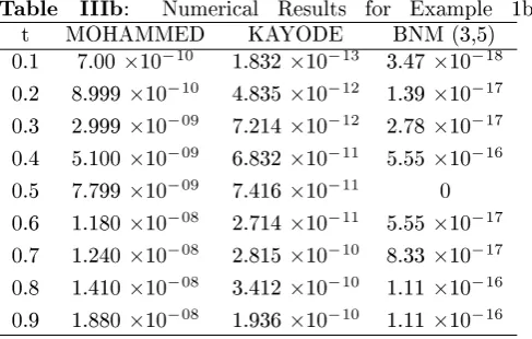
Example 1b: We consider the special fourth order problem (see Kayode [24])

yiv =x,

y(0) = 0, y(0) = 1, y(0) = 0, y(0) = 0 0≤x≤1

whose analytical solution isy(x) = x 2

120 +x.

Example 1b was solved by Kayode et al. and Mo-hammed. The results are compared with the result of B(3,5) which shows its better performance.

Table IIIb: Numerical Results for Example 1b

t MOHAMMED KAYODE BNM (3,5)

0.1 7.00 ×10−10 _1.832×10−13 _{3.47 ×10}−18

0.2 8.999×10−10 _4.835×10−12 _{1.39 ×10}−17

0.3 2.999×10−09 _7.214×10−12 _{2.78 ×10}−17

0.4 5.100×10−09 _6.832×10−11 _{5.55 ×10}−16

0.5 7.799×10−09 _7.416×10−11 ₀

0.6 1.180×10−08 _2.714×10−11 _{5.55 ×10}−17

0.7 1.240×10−08 _2.815×10−10 _{8.33 ×10}−17

0.8 1.410×10−08 _3.412×10−10 _{1.11 ×10}−16

0.9 1.880×10−08 _1.936×10−10 _{1.11 ×10}−16

Example 1c: We consider homogeneous fourth or-der problem (see Awoyemi [7])

yiv = 4y,

y(0) = 1, y(0) = 3, y(0) = 0, y(0) = 16 0≤x≤1

whose analytical solution isy(x) = 1−x+e2x_−e−2x_.

Example 1c was solved by Awoyemi et al. with no comparison of the solution with existing method. Their results are compared with the result of B(5,7).

IAENG International Journal of Applied Mathematics, 49:4, IJAM_49_4_33

Table IIIc: Numerical Results for Example 1c

t AWOYEMI BNM (5,7)

0.1 0 0

0.2 0 2.22 ×10−16

0.3 2.22×10−16 _{4.44 ×10}−16

0.4 2.44×10−15 ₀

0.5 1.15×10−14 _{4.44 ×10}−16

0.6 3.31×10−14 _{8.88 ×10}−16

0.7 7.28×10−14 _{8.88 ×10}−16

0.8 1.37×10−13 _{1.78 ×10}−15

0.9 2.31×10−13 _{3.55 ×10}−15

Example 2: Consider the nonlinear fourth order problem (see Awoyemi [5])

yiv _{= (y)}2_−yy−4t2_+et_{(1 +t}2_−4t),

y(0) =y(0) = 1, y(0) = 3, y(0) = 1 0≤t≤1

whose analytical solution isy(t) =t2+et_.

TableIV∗: Numerical Results for Example 2

h Method Absolute Error at

t=1 0.1 BNM(3,5)

BNM(5,7) BHCM4 ADAMS AWOYEMI

4.76(-13) 4.44(-16) 1.95(-14) 2.44(-6) 9.26(-5) 0.2 BNM(3,5)

BNM(5,7) BHCM4 ADAMS AWOYEMI

3.06(-11) 2.22(-15) 2.38(-12) 5.01(-7) 5.84(-4)

Table 2: Results for Example 2

BNM (3,5) BNM (5,7)

N Err ROC ERr ROC

5 1.26×10−4 _1.35×10−7 10 1.91×10−6 _{6.04 5.12×10}−10 _8.04 20 2.96×10−8 _{6.01 1.93×10}−12 _8.05 40 4.62×10−10 _{6.00 9.95×10}−14 _4.28 80 6.34×10−12 _{6.12 7.11×10}−13 _***

Example 3: This is an application problem from Ship Dynamics which was stated by Wu [35] when a sinusoidal wave of frequency Ω passes along a ship or

oshore structure, the resultant uid actions vary with time t.In a particular case study by Wu etal.[35], the fourth order problem is dened as

yiv+ 3y+y(2 +εcos(Ωt)) = 0,

y(0) = 1, y(0) =y(0) =y(0) = 0, t >0

whereε= 0 for the existence of the theoretical solution,

y(t) = 2 cos t - cos(t√2).The theoretical solution is

undened whenε= 0=0 (see Twizell [32]).

Table V∗: Performance comparison for Wu equation

withε= 0

h Method Absolute Error at

t=15 0.1 BNM(3,5)

BNM(5,7) BHCM4 ADAMS CORTELL

3.4(-10) 0 2.8(-10) 8.4(-5) 3.7(-5) 0.25 BNM(3,5)

BNM(5,7) BHCM4 ADAMS TWIZELL

8.2(-8) 1.7(-11) 5.2(-7) 4.9(-3) 1.9(-4)

Table 3: Results for Example 3

BNM (3,5) BNM (5,7)

N Err ROC ERr ROC

5 1.26×10−4 _1.35×10−7 10 1.91×10−6 _{6.04 5.12×10}−10 _8.04 20 2.96×10−8 _{6.01 1.93×10}−12 _8.05 40 4.62×10−10 _{6.00 9.95×10}−14 _4.28 80 6.34×10−12 _{6.12 7.11×10}−13 _***

Tables 4∗ and 5∗ show the performance comparison

of results between the BNM and the existing Yap and Ismail block hybrid collocation method [36], Adams method, Jator nite dierence method [21] and Awoyemi multi-derivative collocation method [5].The superiority of BNM (5,7) which is of lower order to the order 8 of BHCM4 is established as it more accurate than the existing methods compared with.

Example 4: Consider the linear system (see Hussain

IAENG International Journal of Applied Mathematics, 49:4, IJAM_49_4_33

[19])

yiv_{=u e}3x_{, y(0) = 1, y(0) =−1, y(0) = 1, y(0) =−1.} ziv_{= 16y e}−x_{, z(0) = 1, z(0) =−2, z(0) = 4,}

z(0) =−8.

wiv _{= 81z e}−x_{, w(0) = 1, w(0) =−3, w(0) = 9,} w(0) =−27.

uiv= 256w e−x, u(0) = 1, u(0) =−4, u(0) = 16, u(0) =−64.

The exact solution is given by

y(x) =e−x, z(x) =e−2x, w(x) =e−3x, u(x) =e−4x

The problem is integrated in the interval [0, 2].

This example was chosen to show the performance of BNM(3, 5) and BNM(5, 7) on a system. Looking at Table VI, we deduced that BNM(3, 5) and BNM(5, 7) exhibit an order 5 and 7 respectively, since on halving the step size ofeach method,Erris reduced by a factor

25 or27.

Table 4: Results for Example 4

BNM (3,5) BNM (5,7)

N Err ROC ERr ROC

5 1.21×10−3 _4.74×10−6 10 2.18×10−5 _{5.80 2.13×10}−8 _7.80 20 3.53×10−7 _{5.95 8.64×10}−11 _7.95 40 5.57×10−9 _{5.99 3.44×10}−13 _7.97 80 8.73×10−11 _{6.00 1.78×10}−15 _7.60 80 1.39×10−12 _{5.97 6.57×10}−15 _***

6.2 BVPs

Example 5: We consider the following nonlinear bound-ary value problem in [0, 1], (see [30], [31], [12]).

⎧ ⎪ ⎪ ⎨ ⎪ ⎪ ⎩

y(iv)_{(x) = (y(x))}2_−x10_{+ 4x}9_−4x8_−4x7_{+ 8x}6_−4x4

+120x−48

y(0) = 0, y(0) = 0

y(1) = 1, y(1) = 1

with exact solution y(x) =x5 _2x4 _{+ 2x}2_.

This problem was solved by Noor and Mohyud-Din ([30] [31]) using variational method (NMD method) of approximating polynomial ofdegree 14 and Costabile and Napoli [12] (HBVP method) with polynomial of degree 6. We compare the result ofour method, BNM (3,5) with their results as shown in Table VII.

It is obvious from the numerical results in Table VII that the method is more accurate.

Table VII: Numerical Results for Example 5

t NMD HBVP BNM (3,5)

0.1 4.57×10−16 _{7.35 ×10}−16 _{6.94 ×10}−18

0.2 1.59×10−15 _{2.34 ×10}−15 _{1.39 ×10}−17

0.3 3.16×10−15 _{4.11 ×10}−15 _{2.78 ×10}−17

0.4 4.77×10−15 _{5.83 ×10}−15 _{1.11 ×10}−16

0.5 6.05×10−15 _{5.99 ×10}−15 _{1.11 ×10}−16

0.6 6.66×10−15 _{5.55 ×10}−15 _{1.11 ×10}−16

0.7 6.66×10−15 _{5.21 ×10}−15 _{1.11 ×10}−16

0.8 5.22×10−15 _{3.10 ×10}−15 _{1.11 ×10}−16

0.9 2.55×10−15 _{5.55 ×10}−16 _{1.11 ×10}−16

Example 6 (see [30], [12]) ⎧

⎨ ⎩

y(iv)_{(t) =y(t) +y(t) +e}t_{(t−3), t∈[0,1]} y(0) = 1, y(0) = 0

y(1) = 0, y(1) =−e

Exact solution is y(t) = (1-t)et_.

Table VIII compares the results ofNMD, HBVP and BNM (3,5) methods. Its second and third columns show respectively the error in the NMD and HBVP methods each ofpolynomial ofdegree 15 while the last column contains the error in the BNM (3,5) ofdegree 8.

Table VIII: Numerical Results for Example 6

t NMD _{(degree 15}HBV P ₎ BNM(3,5) 0.1 2.00×10−10 _1.97×10−13 _1.23×10−14 0.2 7.00×10−10 _1.56×10−13 _4.03×10−14 0.3 1.35×10−9 _1.83×10−13 _7.13×10−14 0.4 2.00×10−9 _2.06×10−13 _9.53×10−14 0.5 2.51×10−9 _2.02×10−13 _1.06×10−13 0.6 2.72×10−9 _2.25×10−13 _1.00×10−13 0.7 2.21×10−9 _2.04×10−13 _7.88×10−14 0.8 1.80×10−9 _1.98×10−13 _4.71×10−14 0.9 7.25×10−10 _2.18×10−13 _1.56×10−14

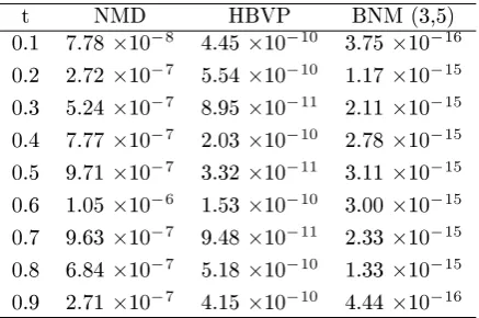
Example 7 (see [30], [12]) ⎧

⎨ ⎩

y(iv)(t) = sint+ sin2t−(y(t))2, t∈[0,1]

y(0) = 0, y(0) = 1

y(1) = sin(1), y(1) = cos(1)

with exact solution y(t) = sin(t)

It was solved by Noor and Mohyud-Din (see [30], [31])

and Costabile and Napoli [12] taking h = 0.1 by using

NMD and HBVP methods of approximating polynomials of degrees 11 and 8 respectively. We also solved for the same step size with our method, BNM (3,5) and the absolute errors at dierent points are shown in Table IX. The superiority of BNM (3,5) is established numerically.

IAENG International Journal of Applied Mathematics, 49:4, IJAM_49_4_33

Table IX: Numerical Results for Example 7

t NMD HBVP BNM (3,5)

0.1 7.78×10−8 _{4.45 ×10}−10 _{3.75 ×10}−16

0.2 2.72×10−7 _{5.54 ×10}−10 _{1.17 ×10}−15

0.3 5.24×10−7 _{8.95 ×10}−11 _{2.11 ×10}−15

0.4 7.77×10−7 _{2.03 ×10}−10 _{2.78 ×10}−15

0.5 9.71×10−7 _{3.32 ×10}−11 _{3.11 ×10}−15

0.6 1.05×10−6 _{1.53 ×10}−10 _{3.00 ×10}−15

0.7 9.63×10−7 _{9.48 ×10}−11 _{2.33 ×10}−15

0.8 6.84×10−7 _{5.18 ×10}−10 _{1.33 ×10}−15

0.9 2.71×10−7 _{4.15 ×10}−10 _{4.44 ×10}−16

7 Conclusion

A family of Nyström type methods BNM (3,5) and

BNM (5,7) have been presented and implemented in a

block-by-block manner to solve fourth order IVPs and BVPs.It has been shown via the numerical examples given in the Section 6 that the methods are accurate and competitive with those given in the literature.Our future research will be focused on extending these methods to solve partial dierential equations via the method of lines.

References

[1] Adesanya, A.O., Momoh, A. A. Alkali, M. A., Tahir, A., Five Steps Block Method For The Solution Of Fourth Order Ordinary Dierential Equations, In-ternational Journal of Engineering Research and Ap-plications, pp.991-998, 2(5)/12

[2] Adeyefa, E.O., Orthogonal-based hybrid block method for solving general second order initial value problems, Italian journal of pure and applied math-ematics, pp.659-672, 37/17

[3] Alomari, A. K., Ratib Anakira, N., Bataineh, A. S., Hashim, I., Approximate solution of nonlinear sys-tem of BVP arising in uid ow problem, Mathemat-ical Problems in Engineering, vol.2013, Article ID 136043, 7 pages, /13

[4] Awoyemi, D.O., A P-stable linear multistep method for solving general third order ordinary dierential equations, International J. Comput. Math., pp.987-993, 80(8)/03

[5] Awoyemi, D.O., Algorithmic collocation approach for direct solution of fourth-order initial-value prob-lems of ordinary dierential equations, International J. Comput. Math., pp.321-329, 82(3)/05

[6] Awoyemi, D.O., Adebile, E. A., Adesanya, A.O., Anake, T.A.: Modied block method for the direct

solution of second order ordinary dierential equa-tions. International Journal of Applied Mathematics and Computation, pp.181-188, 3(3)/11

[7] Awoyemi, D.O., Kayode, S.J., Adoghe, L.O., A six-step continuous multisix-step method for the solution of general fourth order initial value problems of or-dinary dierential equations Journal of Natural Sci-ences Research , pp.131-138, 5(5)

[8] Boutayeb, A., Chetouani, A., A mini-review of nu-merical methods for high-order problems. International Journal of Computer Mathematics, pp.563 -579, 84(4)/07

[9] Bun, R. A., Varsolyer, Y. D., A numerical method for solving dierential equation of any orders, Com-put. Math. Phys., 317-330, 32(3)/92

[10] Butcher, J.C., Numerical Methods for OrdinaryDif-ferential Equations, Second Edition, John Wiley and Sons Ltd., England, 2008.

[11] Cortell, R., Application of the fourth-order Runge-Kutta method for the solution of high-order general initial value problems, Computers and Structures, pp.897-900, 49(5)/93

[12] Costabile, F., Napoli, A., Collocation for high or-der dierential equations with two-points Hermite boundary conditions, Applied Numerical Mathemat-ics, pp.157-167, 87/15

[13] Dormand, J.R., Numerical Methods for Dierential Equations. A Computational Approach, CRC Press, Inc., Florida, 1996.

[14] Fatunla, S.O., Numerical Methods for initial value problems for ordinarydierential equations, U. S. A Academy press, Boston, p.295, 1988.

[15] Fatunla, S.O., Block method for second order ini-tial value problem (IVP), International Journal of Computer Mathematics, 55-63, 41/91

[16] Fatunla, S.O., A class of block methods for second order IVPs, Int. J. Comput. Math., 119-133, 55/94 [17] Hairer, E., Norsett, S.P., Wanner, G., Solving

Or-dinaryDierential Equations I: Non-sti Problems, Springer-Verlag, Berlin, 1993.

[18] Henrici, P., Discrete Variable Methods in Ordinary Dierential Equations, John Wiley and Sons Ltd., New York, 1962.

[19] Hussain, K. Ismail, F., Senua, N., Solving directly special fourth order ordinary dierential equations using Runge Kutta type method, Journal of Com-putational and Applied Mathematics, pp.179-199, 306/16

IAENG International Journal of Applied Mathematics, 49:4, IJAM_49_4_33

[20] Jator, S.N., A Sixth Order Linear Multistep Method for the Direct Solution of y=f(x,y,y'), International Journal of Pure and Applied Mathematics, PP. 457-472, 40(4)/07

[21] Jator, S.N., Numerical integrators for fourth order initial and boundary value problems, International Journal of Pure and Applied Mathematics, pp. 563 -576, 47(4)/08

[22] Kayode, S. J., An order six zero-stable method for direct solution of fourth order ordinary diferential equations, American Journal of Applied Sciences, pp. 1461-1466, 5(11)/08

[23] Kayode, S. J., An ecient zero-stable numerical method for fourth-order diferential equations, Inter-national Journal of Mathematics and Mathematical Sciences, doi: 10: 1155/2008/364021, /08

[24] Kayode, S. J., Duromola M.K., Bolarinwa B., Di-rect Solution of Initial Value Problems of Fourth Or-der Ordinary Dierential Equations Using Modied Implicit Hybrid Block Method, Journal of Scientic Research and Reports, pp. 2792 - 2800, 3(21)/14

[25] Lambert, J.D., Numerical Methods for Ordinary Dif-ferential Systems, Wiley, Chichester, (1991).

[26] Lambert, J.D., Computational methods for ordinary dierential equations, John Wiley, New York, 1973.

[27] Malek, A., Beidokhti, R. S., Numerical solution for high order diferential equations using a hybrid neural network-optimization method, Applied Mathematics and Computation, pp. 260-271, 183(1)/06

[28] Mehrkanoon, S., A Direct Variable Step Block Multi-step Method for Solving General Third-Order ODEs. Numerical Algorithms, pp. 53-66, 57(1)/11

[29] Mohammed U., A six step block method for solution of fourth order ordinary dierential equations. The Pacic Journal of Science and Technology, pp. 258-265, 11(1)/10

[30] Noor, M.A., Mohyud-Din, S.T.: An ecient method for fourth order boundary value problems. Comput. Math. Appl., pp. 1101-1111, 54/07

[31] Noor, M.A., Mohyud-Din, S.T., Variational itera-tion technique for solving higher order boundary value problems. Appl. Math. Comput., pp. 1929-1942, 189/07

[32] Twizell, E.H., A family of numerical methods for the solution of high-order general initial value problems, Computer Methods in Applied Mechanics and Engi-neering, pp. 15-25, 67(1)/98

[33] Vigo-Aguilar, J., Ramos, H., Variable step size implementation of multistep methods for y =

f(y, y, y). J. of comput. Appl. Math., pp. 114-131,

192/06

[34] Waeleh, N., Majid, Z.A., Ismail, F., Suleiman, M.: Numerical solution of higher order ordinary dieren-tial equations by direct block code, J. Math. Stat., pp. 77-81, 8(1)/12

[35] Wu, X. J., Wang, Y., Price, W. G.: Multiple resnances, responses, and parametric instabilities in o-shore structures, Journal of Ship Research, pp. 285 - 296, 32(4)/88

[36] Yap, L.E., Ismail. F.: Block Hybrid Colloca-tion Method with ApplicaColloca-tion to Fourth Or-der Dierential Equations, Mathematical Prob-lems in Engineering, Article ID 561489, 6 pages, doi:10.1155/2015/561489, 2015/15

IAENG International Journal of Applied Mathematics, 49:4, IJAM_49_4_33