Curve and Polygon Evolution Techniques for Image Processing

(1)

ABSTRACT

BOZKURT, GOZDE. Curve and Polygon Evolution Techniques for Image Processing.

(Under the direction of Dr. Hamid Krim.)

In this digital era of our world, huge amounts of digital image data are being collected on a daily

basis. The collected image data is being stored for subsequent processing and use in a wide variety

of applications. For this purpose, it is often important to accurately and precisely extract relevant

information out of this data. In computer vision applications, for instance, an important goal is to

understand the contents of an image and be able to automatically gain an understanding of a scene,

implying an extraction and recognition of an object. This task is, however, greatly complicated by

the acquired image data being often noisy, and target objects and background bearing textural

varia-tions. As a result, there is a strong demand for reliable and automated image processing algorithms,

for image smoothing, textured image segmentation, object extraction, tracking, and recognition.

The objective of this thesis is to develop image processing algorithms which are efficient,

statisti-cally robust and sufficiently general, in order to account for noise and textural variations in images,

and which have the ability to extract and provide compact and useful descriptions of target objects

in images, for object recognition and tracking purposes.

The main contribution of the thesis is the development of image processing algorithms, which

are based on the theory of curve evolution with connections to information theory and

probabil-ity theory. These connections form the basis for extracting a compact object description, in the

form of a polygonal contour. One contribution is the development of a new class of curve

evo-lution equations designed to preserve prescribed polygonal structures in an image while removing

noise. In conjunction with these flows, a local stochastic formulation of a well-studied curve

evo-lution equation, namely the geometric heat equation, provides an alternative microscopic as well as

macroscopic view, which in turn led to our proposal of vanishing at pre-defined directions. Under

these flows, the limiting shape of a curve is a polygon, pre-specified by the form and the parameters

of the specific flow. The second contribution of the thesis is the development of a new active

con-tour model which merges the desirable polygonal representation of an object directly to the image

segmentation procedure by adapting an information-theoretic measure into an active contour

frame-work with an ultimately unsupervised texture segmentation goal. The polygon-propagating models

we develop can capture texture boundaries more reliably than the continuous active contour models

(2)

along its two adjacent polygon edges rather than on pointwise measurements along continuous

con-tour points. In this way, higher-order statistics which provide more adapted information than the

first and second-order, are captured through both the nature of the information-theoretic criterion

we utilize, and the nature of the polygon-evolving ordinary differential equations we propose. A

supplementary contribution in this sequel is a new global polygon regularizer algorithm which uses

electrostatics principles. The final contribution of the thesis is the development of a simple and

efficient boundary-based object tracking algorithm well-adapted to polygonal objects. This is an

extension of the second contribution of the thesis, and the key idea here is centered around tracking

a relatively few vertices together with their corresponding edges, which in turn yields a bookkeeping

simplicity and hence efficiency.

The parsimonious set of features provided by the three methods developed in this thesis are

use-ful for object-based description and recognition tasks, and in addition, may provide a viable solution

to a parsimonious, and economical representation of large data sets (e.g. a contour represented by a

(3)

(4)

(5)

Biography

G ¨ozde Bozkurt ¨Unal completed her high school education at Ataturk Anadolu Lisesi, Ankara, in

1992, and received her Bachelor of Science degree in Electrical and Electronics Engineering with

High Honors from Middle East Technical University, Ankara, Turkey, in 1996. She started her

grad-uate studies at Bilkent University, Ankara, in 1996, and worked on digital halftoning problems, new

error diffusion techniques using adaptive filtering, and inverse halftoning techniques. She earned

her Master of Science degree in Electrical and Electronics Engineering from the Bilkent University,

Ankara, Turkey, in 1998.

Since August 1998, she continued her graduate studies in the Electrical and Computer

Engineer-ing Department at North Carolina State University, Raleigh, NC, and worked as a research assistant

at the Vision, Information and Statistical Signal Theories and Applications group, pursuing her

Ph.D. degree. Her research interests include curve evolution theory with connections to information

theory and probability theory, application of curve evolution techniques to various image and video

processing problems such as image smoothing, image and texture segmentation, object tracking,

(6)

Acknowledgments

In making this work possible, I would like to express my gratitude to:

Dr. Hamid Krim, for his supervision, guidance, financial support through grants from AFOSR,

and ONR-MURI; his mentoring towards unexplored and challenging topics, relaying to his students

an appreciation for mathematics, and always having an open door for discussions.

Dr. Anthony Yezzi, for his co-supervision, invaluable support and guidance, his insights and

ideas, and valuable discussions.

Dr. Kazufumi Ito of the Mathematics Department, for his encouraging comments, and support,

and serving on my committee.

Dr. Wesley E. Snyder, and Dr. Gianluca Lazzi, members of my committee, for being interested

in this work, and their comments.

Dr. Jean-Pierre Fouque of the Mathematics Department through his enlightening class on SDEs,

and for his help and comments; Dr. Yufang Bao for fruitful discussions and suggestions on this

topic.

Group and office mates, Dr. A. Ben Hamza and Oleg Poliannikov, for heated discussions on

research and life in general, and humorous moments.

Sandy Bronson, our administrative assistant, for being so nice and kind, and making things

smoother in arranging official matters, travels, and paperwork.

My parents, Zerrin and G ¨uner Bozkurt, for their sincere love, enormous support and enthusiasm

for my education.

Alper ¨Unal, my beloved husband, who shared with me the pains and the happiness during the

(7)

List of Figures

2.1 Depiction of a level set formulation versus a parametric formulation of a curve. . . 14

2.2 A piece-wise constant image consisting of two regions. . . 20

3.1 Illustration of averaging behaviour. Illustration of averaging behaviour. Points of

the zero-level set, i.e. initial contour (X(t);Y(t)), at timet, is shown on the left. . . 31

3.2 Symmetric random walk on the tangent direction, and corresponding interpolation

on square grid. . . 31

3.3 Generator of symmetric random walk on the tangent direction implemented on the

level set functionu(x;y)for a T shape. . . 32

3.4 Middle row: Generator of symmetric random walk onT is shown to produce

simi-lar results with those in Bottom Row: Geometric Heat flow . . . 33

3.5 Morphing of a circle into different shapes by the given flows is demonstrated. . . . 37

3.6 (a) Initial set of shapes (b) FlowC t

=cos 2

(2)N (c) FlowC t

=sin 2

(2)N. 38

3.7 (a) Initial set of shapes (b)Flow C t

= cos 2

(3)N, which tends to produce

hexagons, (c)FlowC t

=sin 2

(1:5( =2))N, which tends to produce

triangle-like shapes. . . 38

3.8 Each row corresponds to a curve evolution method with different n,1 st

row:C t

=

N,2

nd

row:C t

=sin 2

(2)N,3

rd

row:C t

=cos 2

(4)N. . . 40

row:C t

=

N,2

nd

row:C t

=cos 2

(2)N,3

rd

row:C t

=sin 2

(4)N. . . 41

row:C t

=

N,2

nd

row: C t

= sin 2

(1:5( =2))N, 3

rd

row: C t

= sin 2

(2)N,4

th

row:C t

=cos 2

(11)

3.11 (a) Clean building image (b) noisy building image (c) Geometric heat flowu t

=u

(left-right)t=10;20;40(d) Flowu t

=cos 2

(2)u

(left-right)

t=10;20;40. . . 45

3.12 (Top) Diamonds image (Middle row) Geometric heat flowu t

= u

(Bottom row)

Flowu t

=sin 2

(2)u

. . . 46

3.13 (Top) An image from mars pathfinder, (First column) Geometric heat flowu t

=u ,

(Second column) Flowu t

=cos 2

(3)u

. (Image: Origin NASA, exposed by and

courtesy of N. Coombs & NPAAG 1998.) . . . 47

3.14 Top: Aerial image; 2 nd

row: geometric heat flow u t

= u

, (left to right)

t =

20;40;80;3 rd

row: flowu t

=cos 2

(2)u

, (left to right)

t=20;40;80. . . 48

3.15 Top: House; Left: Geometric heat flowu t

=u

, (top to bottom)

t =40;80;160;

Right: Flowu t

=cos 2

(2)u

, (top to bottom)

t=40;80;160. . . 49

4.1 Motivational example where a simple binary image containing a quadrilateral (at

the top) with additive uniform noise is to be segmented. First three rows show

a continuous active contour propagation with small, medium, large regularization

respectively. . . 55

4.2 We demonstrate flow (4.6) for two different initial active polygons. . . 63

4.3 A continuous contour with a small regularization (top row), fails to capture as a

whole an object with a synthetic texture of vertical stripes , whereas with a large

reg-ularization (middle row), rounds off the boundaries, and continues to shrink without

sticking to the data. A polygonal contour (bottom row) correctly segments the

tex-tured region. . . 68

4.4 An active contour (first row) fails to capture synthetic texture of vertical stripes even

after a Gabor filtering, whereas the active polygon (second row) captures the outline

of the textured region. . . 69

4.5 Ternary image regions. . . 70

4.6 Ternary flows using image forces withG(x)= x, are used to segment this simple

ternary image corrupted by Gaussian noise. . . 73

4.7 We demonstrate that flow (4.6) may become degenerate without an additional

con-straint on the motion of vertices. . . 74

4.8 Calculation of electric force exerted by a line charge (a;b) at a point x 0

on the

(12)

4.9 Electrostatic regularizer in Eq.(4.32) computes the electric force at each vertex. . . 76

4.10 The electric forces for an evolution are shown. Note the forces only become signif-icant when a vertex approaches another vertex or edge. . . 77

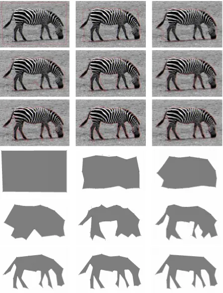
4.11 A zebra figure is captured by the active polygon model. A generic rectangular active polygon close to image boundaries is initialized. . . 80

4.12 A monarch larvae on a leaf is captured by an active polygon (left). Monarch butterfly is captured in the two other columns with very different initalizations. . . 81

4.13 A fish with a striped texture is captured. . . 82

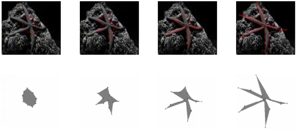
4.14 A sea star embedded in a textured rocky background is captured. . . 82

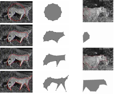
4.15 Left: Cheetah figure is captured by the active polygon. Right: A cheetah in bushes is captured with an active polygon. . . 83

4.16 A natural crystal chunk is captured. . . 83

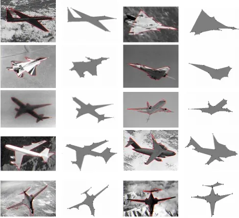
4.17 Each airplane is captured by a handful of vertices. . . 85

4.18 A submarine figure is captured by a handful of vertices. . . 86

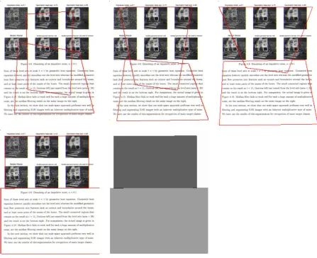
4.19 An active polygon nicely segments a document image scanned from an article. . . . 86

4.20 Two active polygons capture text and image regions of a page from an article. . . . 87

5.1 The Aperture Problem . . . 92

5.2 2-D velocity field along two neighbor edges of a polygon vertex. . . 94

5.3 Tracking of an IR image sequence I. . . 97

5.4 Tracking of an IR image sequence II. . . 98

5.5 Tracking of an IR image sequence III. . . 99

5.6 Tracking of an IR image sequence IV. . . 100

5.7 Tracking of another IR image sequence V. . . 101

5.8 Tracking of a toy airplane moving on a conveyor belt . . . 102

5.9 Tracking of a model rocket object. . . 102

5.10 Tracking of the black automobile entering the scene. . . 103

5.11 Tracking of a truck approaching from the far left. . . 103

5.12 Intra-class Image Retrieval Scenario. . . 107

5.13 Set of airplane images under different conditions. . . 108

5.14 An airplane from two different views. . . 110

(13)

5.16 The next-to-top matches are shown for the test airplane in Fig. 5.15. . . 112

5.17 A query, which is an F16, to model image set, and a top match are shown. . . 112

5.18 The next-to-top matches are shown for the test airplane in Fig. 5.17. . . 113

5.19 Outputs of several random initializations for F16 airplane. . . 113

5.20 Average turning function versus arc length over eight different realizations shown in Fig.5.19. . . 114

(14)

Chapter 1

Introduction

In this digital era of our world, huge amounts of digital image data are being collected on a daily

basis. The collected image data is being stored for subsequent processing and use in a wide variety

of applications. For surveillance applications for instance, the amount of remotely sensed imagery

collected daily by space-borne or airborne systems is on the order of terra bytes. It is often important

to accurately and precisely extract relevant information out of this data for a variety of applications.

It is, however, impossible to manually carry out this processing and analysis wholly by human

op-erators. The acquired image data is often noisy, and target objects and background bear significant

textural variations. It may also be desirable to track features or objects in an image through time to

obtain a dynamic analysis of the scene. In computer vision applications, for instance, an important

goal is to understand the contents of an image and be able to automatically gain an understanding

of the scene and the surroundings, implying an extraction and recognition of an object. As a

re-sult, there is a strong demand for reliable and automated image processing algorithms, for image

smoothing, textured image segmentation, object tracking in video sequences, and object extraction

and recognition.

The broad objective of this thesis is that of developing image processing algorithms which are

efficient, in the sense of ease of computations, fast, statistically robust, in the sense of being resilient

to noise, statistically significant and meaningful, in the sense of accounting for textural variations in

images, with an ability to extract and provide compact and useful descriptions of target objects in

images, for object recognition and tracking purposes.

We next give the motivations for the image processing algorithms we developed, which

(15)

thesis.

1.1 Thesis Motivations and Contributions

Curve evolution techniques for image processing involve a propagation or deformation of a curve via

certain partial differential equations (PDEs). Curve evolution techniques are applied to a variety of

problems, such as image filtering, smoothing, image segmentation, object tracking, shape analysis,

and morphological operations. The main contributions of this thesis are, first the development of

a new class of curve evolutions as nonlinear filters for curve and image smoothing, second the

development of a new class of curve evolutions, where the curve takes the form of a polygon for

image segmentation, and which makes use of an information-theoretic measure adapted to texture

segmentation. A third contribution of the thesis is the extension of the second algorithm that is

developed in Chapter 4 to object tracking in video sequences. Potential applications of the proposed

algorithms in shape or object recognition are also alluded to.

The motivation and contribution of each of these algorithms are described in the next three

subsections.

1.1.1 A New Class of Curve Evolutions for Nonlinear Filtering

Curve and image evolution techniques have emerged in recent years as important applications of

PDEs to nonlinear curve and image filtering. The well-known low-pass filtering of an image by a

Gaussian function has been shown by Witkin [147] to be equivalent to evolving an image with a

heat equation, which is a linear PDE also known as a linear diffusion. This in turn lead to

vari-ous developments in nonlinear filtering of images through numervari-ous PDEs and nonlinear diffusion

techniques [6, 110, 117, 122, 136]. In addition to these developments in image filtering, the advance

of curve evolution techniques may be considered as an implication of the desire to develop

shape-based techniques, which is closer in spirit to providing object level knowledge in image analysis.

Image evolution equations operate on a pixel-based knowledge, whereas curve evolution equations

operate on individual level curves of an image, hence at a higher level than the former. Shape

infor-mation of an object in an image, may be reminiscent of a curve extracted from an image, thus for

an object-oriented filtering, curve evolutions may be more appropriate.

Much of the research in curve evolution theory has centered around the so-called geometric heat

(16)

geometric heat equation is circularized [54]. One way of overcoming this effect is by using prior

information on the preferred directions of important features of objects in an image. Polygonal

structures are ubiquitous in images of man-made objects such as buildings, roads and so on, which

contain many straight lines, often oriented in particular directions.

The first contribution of this thesis is the development of curve evolution techniques which

constitute a new class of nonlinear filters aimed for smoothing along salient lines of an image. These

filters which act on level curves preserve sharp corners, and hence preserve the polygonal structures

present in an image. This is achieved by a modification, indeed a directional generalization, of

the celebrated geometric heat equation. The designed equations or flows preserve certain classes

of features in a curve. This, followed a local stochastic formulation of the geometric heat flow,

leading to a new macroscopic view of this equation, which is later further specified to vanish at

pre-defined directions. The limiting shape resulting from each flow that belongs to the new class

of curve evolving flows is a polygon, pre-specified by the form and the parameters of the specific

flow. When applied to an image, a selective nonlinear filtering along the salient lines in the image

is achieved slowing down the effects of geometric diffusion across important structural directions.

This new class of filters are presented in Chapter 3.

We have also developed a variant of this contribution, for smoothing a group of level curves

of synthetic aperture radar (SAR) imagery, which is particularly robust to speckle noise typically

present in SAR images. These curve evolutions, which lead to a simple segmentation of SAR

images and target recognition on the extracted silhouettes, are presented in [140, 142].

1.1.2 A Polygon Evolution Approach to Image and Texture Segmentation

Image segmentation has received a lot of attention through the years, and a vast array of

differ-ent approaches have been proposed, such as thresholding and local filtering [22, 97, 112, 134],

re-gion growing [100], snakes, and active contours [25, 34, 70, 72, 93], and global energy

minimiz-ing techniques usminimiz-ing various perspectives such as Bayesian, and minimum description length [17,

51, 87, 102]. Following the pioneering snake methodology [70], curve evolution approaches,

so-called active contours, have been popular in image segmentation. The key idea in the active

con-tour framework is the construction of an energy functional for the active concon-tour, and its

min-imization through the gradient descent equations that propagate the active contour. Two main

categories of active contour methods are given by; geometric (also called geodesic) active

(17)

active contours [29, 115, 121, 150], where the curve evolution is based on the region information

inside and outside the curve.

The region-based active contour models proved to be more robust to noise conditions when

compared to edge-based active contour models. The region-based model usually utilizes simple

region statistics such as means and variances, hence can not account for higher order nature of

the textural characteristics of image regions. In addition, the object delineation by active contour

methods, results in a contour representation which still requires a substantial amount of data to be

stored for subsequent multimedia applications such as visual information retrieval from databases.

Polygonal approximations of the extracted continuous curves are required to reduce the amount of

data since polygons are powerful approximators of shapes for use in later recognition stages such

as shape matching and shape coding.

The second contribution of this thesis is the development of a new active contour model which

nicely ties the desirable polygonal representation of an object directly to the image segmentation

process by including an information-theoretic measure into the active contour framework with an

unsupervised texture segmentation goal. The polygon-propagating models we develop can robustly

capture texture boundaries relative to the continuous active contour models as the evolution of an

active polygon vertex depends on an overall speed function integrated along its two adjacent

poly-gon edges rather than pointwise measurements along continuous contour points. In this way, more

higher-order statistics than the first and second-order are rationally captured through the proposed

information-theoretic measure we utilize, and the nature of the polygon-evolving ordinary

differen-tial equations we derive. This new variational texture segmentation model, is unsupervised since

no prior knowledge on the textural properties of image regions is used, and will be described in

Chapter 4.

A by-product, nevertheless necessary, contribution in this sequel is a new polygon regularizer

algorithm which uses electrostatics principles. This is a global regularizer, and is more consistent

in preserving local features such as corners than a local polygon regularization, as is explained in

Section 4.5.

1.1.3 A Polygon Propagation Approach to Video Object Tracking

Video sequences, i.e. time-varying image sequences, provide additional information on how scenes

and objects change over time when compared to still images. The problem of tracking moving

(18)

robotics. Object tracking methods, may be classified into two categories according to the type of

information they use. Boundary-based methods, which utilize the boundary information along the

object’s contour, make use of snake models [12, 67, 70, 89], or geometric active contour models [24,

114], and usually constrain motion by certain motion models such as rigid or affine. Region-based

methods [9, 10, 145] segment an image sequence into regions (with different motions), which are

matched to estimate motion. The cost of matching regions significantly increases the computational

burden of these techniques.

The third contribution of this thesis is the development of a simple and efficient boundary-based

tracking algorithm well-adapted to polygonal objects. We build on the insight gained from the

the second contribution of the thesis, namely the active polygon framework, to extend it to track

polygon vertices in time-varying images. The key idea here is centered around tracking a relatively

few vertices together with their corresponding edges, which in turn yield a simplicity and efficiency

in bookkeeping. This object tracking method, together with an experimental study of applying

active polygons to an object recognition scenario, are presented in Chapter 5.

1.1.4 Connections Among the Contributions

The three main contributions of this thesis may be cast within a unified objective of extracting a

compact object description, in the form of a polygonal contour, which leads to an efficient

repre-sentation of an object crucial to subsequent computer vision applications. The first contribution, in

Chapter 3, aims at removing unwanted perturbations on curves while preserving salient features. It

drives a curve (a level curve of an image), which is assumed to contain shape information of an

ob-ject in an image, towards a polygon by straightening the curve out. Inspired by these filters designed

for image smoothing, we proceed to a direct polygonal description of an object in an image with a

resulting segmentation, which is the second contribution of this thesis, in Chapter 4. This compact

description of an extracted object by a handful of vertices, in turn leads to the idea of tracking these

features in a time-varying image sequence, as elaborated in Chapter 5. This contribution may also

be viewed as a generalization or extension of that of Chapter 4.

The parsimonious set of features provided by the three methods developed in this thesis, are

use-ful for object-based description and recognition tasks, and in addition, may provide a viable solution

to a parsimonious, and economical representation of large data sets (e.g. a contour represented by a

(19)

1.2 Thesis Summary and Organization

In Chapter 2 we provide a background on the techniques and concepts that are relevant throughout

this thesis. A review on image and curve evolution techniques is presented in Section 2.2, and the

corresponding numerical implementation technique is given in Section 2.2.3. A brief review of the

literature on segmentation methods is presented in Section 2.3. Snakes, and active contour models

that are related to the algorithms developed in this thesis are introduced in Section 2.3.3.

Chapter 3 describes a new class of curve evolutions developed for feature-preserving curve

and image filtering with a prior knowledge on the salient line directions of objects in an image.

The theory of stochastic differential equations (SDEs) is briefly introduced in Section 3.3.1, and a

formulation of the celebrated geometric heat equation by a local SDE, and thus obtaining a new

microscopic/macroscopic view of this equation, is derived in Section 3.3.2. The insight led to

de-signing a new class of nonlinear filters in the form of diffusions that vanish at pre-defined directions

as explained in Section 3.4. These diffusions on curves yield a limiting polygon shape prescribed by

the parameters of the flow. We have applied this algorithm to smoothing of structures along known

orientation of salient lines in an image while preserving important features. We suggest further

ap-plications of the proposed flows in Section 3.5 such as a shape morphing application in computer

graphics and a shape recognition scenario.

In Chapter 4, we present a new class of variational active contour models for an unsupervised

texture segmentation problem. A brief literature review on texture analysis and segmentation is

given in Section 4.2.1. Through a combination of a novel polygon evolution model in Section 4.3,

and an information-theoretic criterion adapted as an energy functional for the active polygons in

Section 4.4, a robust texture segmentation algorithm is developed as validated through extensive

simulation results provided at the end of Chapter 4. A generalization of the proposed active contour

model to evolution of multiple active contours is also given. Section 4.5 presents a novel global

polygon regularizer idea with a goal of avoiding degeneracy during propagation of the active

poly-gons.

Chapter 5 extends the active polygons acting on a single image to time-varying image sequences,

and presents a video object tracking method in Section 5.1, with an application to tracking targets in

infra red (IR) image sequences. A brief overview on object tracking methods, and motion estimation

methods are also given respectively in Section 5.1.1, and Section 5.1.2. We further demonstrate the

(20)

Section 5.2. This may be considered as part of future research based on the framework set in this

thesis.

(21)

Chapter 2

Preliminaries

This chapter focuses on the background of techniques and concepts that are of relevance throughout

this thesis.

2.1 Notation

A digital image to be processed is a 2-Dimensional (2-D) function denoted byI,I :!R, where

R

2

is the domain of the function. Processing a functionI o

(x;y), which depends on two spatial

variables,x2R, andy2R, via a partial differential equation (PDE) takes the form;

I t

= A(I;I x

;I y

;I xx

;I xy

;I yy

) (2.1)

I(0;x;y) = I o

(x;y):

Heretis called the time or scale.I

tdenotes the partial derivative with respect to (w.r.t.)

t(sometimes

shown as @I @t

), and partial derivatives w.r.t. spatial variables are shown inside the operatorAon the

right hand side. The solutionI(t;x;y)is referred to as a scale space for0<t<1. IfAis a linear

(nonlinear) operator, the scale space is called linear (nonlinear).

Definitions of some operators that are commonly invoked in PDE’s often used in computer

vision are given next. The gradient ofI(t;x;y)is a two-dimensional vector (2-D vector) defined as

rI

def

= (I x

; I y

) T

(22)

where the superscript T denotes the transpose of a vector. TheL

2norm of the gradient is given by

jjrIjj

def

= q

I 2 x

+I 2 y

: (2.3)

Vector fields arise when the gradient operatorris applied to a scalar function such asI(x;y). The

divergence of any vector field(I(x;y); J(x;y)) T

is

r 0

@ I

J 1

A

def

= I

x +J

y

: (2.4)

The Laplacian operator acting on a 2-D function is defined asI =I xx

+I

yy. It is clear that

the Laplacian can also be written as I = rrI. Throughout the thesis, an inner product (dot

product) is denoted by either<;>, or by a dot . The area of a regionRis denoted byjR j. A

boldface letter is used to denote both a vector and a matrix.

Some background on curve and image evolution techniques, and an overview of image

segmen-tation techniques are presented in the following sections.

2.2 Image and Curve Evolution Techniques

Obtaining a family of images (curves) from an initial image (curve) through a PDE is referred to as

an evolution of the image (curve) through timet. It is equivalent to the scale space concept defined

in the previous section. We look at some well-known evolution equations for images and curves

next.

2.2.1 Image Evolutions

It is known that a low pass Gaussian filter from signal processing may be implemented by evolving

the intensities of an imageI o

(x;y)via the linear heat equation [147],

I(0;x;y) = I o

(x;y);

I t

(t;x;y) = r rI(t;x;y)

; t>0: (2.5)

The solution to this equation yields a parameterized family of new images I(t;x;y), where the

image at each timet>0is equivalent to the original imageI 0

(23)

Gaussian filter of variance2t. This equivalence gives rise to a natural generalization of the low pass

filter using nonlinear diffusion.

Nonlinear diffusion has a distinct advantage in image processing over linear diffusion in that

it may be allowed to handle anisotropies (giving rise to the so-called anisotropic diffusion) in an

image.

A popular approach to anisotropic diffusion is based upon models first introduced by Perona and

Malik in [117]. Since then, these models have received a tremendous amount of attention, as have

the models based upon curve evolution theory. Perona and Malik extended the linear heat equation

by considering diffusion coefficients which vary with the strength of the gradient at different points

of an image. This leads to PDE’s of the formI t

=r g(krIk)rI

, whereg:R !R is typically

a monotonically decreasing function which suppresses diffusion where the gradient is high (near an

edge).

Nonlinear diffusion is particularly important when salient image features are of interest. For

example, when the preservation of sharp edges is important, it is natural to consider an anisotropic

model which diffuses an image only along the local direction of its edges. One such approach is to

consider an imageI(x;y)as a collection of iso-intensity contours, or level curves, and to note that

at an edge point, the direction of the edge corresponds to the tangent of the iso-intensity contour

running through that point. Let denote the direction normal to the level curve through a given

point (the gradient direction), and letdenote the tangent direction.

We may write these directions in terms of the first derivatives of the image as

=

(I x

;I y

) q

I x

2 +I

y 2

; =

( I y

;I x

) q

I x

2 +I

y 2

;

Since these constitute orthogonal directions, we may exploit the rotational invariance of the

Lapla-cian operator and re-write the linear heat equation in terms of these two variables:

I t

=r(rI)=I

+I

whereI

and

I

denote the second-order directional derivatives in the directions of

(24)

re-spectively. One may then derive the following expressions I = I 2 x I xx +2I x I y I xy +I 2 y I yy I 2 x +I 2 y (2.6) I = I 2 y I xx 2I x I y I xy +I 2 x I yy I 2 x +I 2 y : (2.7)

By subtracting the normal diffusion component (2.6) from the linear heat equation, which diffuses

isotropically, we obtain the following anisotropic model, which diffuses along the boundaries of

image features but not across them

I t =I = I 2 y I xx 2I x I y I xy +I 2 x I yy I 2 x +I 2 y : (2.8)

We may obtain this same equation in a completely different and much more geometric manner by

specifying the evolution of each level curve in the image as seen in the next section.

2.2.2 Curve Evolutions

Let us denote a family of smooth curves C(p;t) = (X(p;t);Y(p;t)), which is a mapping from

I R[0;T]!R 2

, wherep2Iis a parameter along the curve, andtparameterizes the family

of curves. Denote the tangent vector to the curve at pby T = C 0

= (X 0

;Y 0

), and the normal

vector to the curve atp byN = ( Y 0

;X 0

). We consider regular curves whose tangent is never

zero (C 0

(p)6=0for allp2I).

Givenp2I, the arclength of a regular parameterized curveC from the pointp

ois by definition

s(p)= Z p po jjC 0 (p)jjdp; (2.9) where jjC 0 (p)jj = p (X 0 (p)) 2 +(Y 0 (p)) 2

is the length of the vectorC 0

[41]. Hence ds=dp =

jjC 0

(p)jj.

The most general deformation of a planar curveC o

is given by

@C

@t

= (p;t)T +(p;t)N; (2.10)

C(p;0) = C

o

(p): (2.11)

(25)

@C(p;t) @t

=(p;t)N:Considering curve evolutions which depend only on the curvature function

of the curve, can be written asF(), and a local deformation as a function of curvature may be

written as

C t

=F()N : (2.12)

The curvature function is the second derivative of the curveC, in the direction of the unit normal

N. If the curve is parameterized by its arclength parameter s, the second derivative is given by

C ss

=N. The following flow

C t

=C

ss

=N; (2.13)

referred to as the Geometric Heat Equation (GHE), is well known for its smoothing properties. It

has been shown by Grayson [54] that any closed, embedded curve evolving according to (2.13) will

convexify and smoothly shrink to a single point in finite time, becoming more and more circular

along the way. This flow is also referred to as the curve shortening flow since it corresponds to the

gradient (descent) evolution of the arclength functional. See [74–76] for a more extensive discussion

of the many properties associated with this flow. Since the evolution speed is a function of the

curvature at each point on a curve, this flow gives rise to a Euclidean invariant scale space (see [5,

6, 147]) in which finer features are removed first, followed by coarser features, as the curve evolves.

A related flow, based upon the affine geometry of the curve, is given byC t

=

1=3

N and shares

many of the same properties as the curve shortening flow but gives rise to a more general affine

invariant scale space (see [5, 124, 125]).

2.2.3 Level Set Method

A new and efficient method for evolving a single iso-intensity contour has recently been proposed,

referred to as a level set method [126]. The parameterized curveC(p;t)is embedded into a surface,

which is called the level set function(x;y;t): R 2

[0;T]7! R. The curveC is the zero-level

set of this function(x;y;t):

C =f(x;y):(x;y;t)=0g: (2.14)

The evolution equation for(x;y;t) is derived from the constraint that at any timet, we should

(26)

get t + x X t + y Y t

= 0; (2.15)

t +( x ; y )( X

t Y

t )

T

= 0; (2.16)

t

+rC

t

= 0: (2.17)

Substituting the general form of the curve evolution equation Eq.(2.12), which depends on local

geometry of the curve, into Eq.(2.17) above yields,

t

+rF()N =0: (2.18)

Noting that the outward unit normal vector can be written as, N = r=jjrjj, an evolution

equation foris given by

t

= F()jjrjj: (2.19)

Thus, the curveC evolving according to Eqn (2.12) can be obtained by the zero-level set of the

function which evolves according to Eqn (2.19). The selection of the speed functionF()has

been a subject of research [126]. The simplest form whereF()= results in

t

=jjrjj: (2.20)

Note that the unit normal and the curvature of a level curve may be expressed asN = r krk and = r r krk

. This allows us to rewrite the above equation completely in terms ofand its

derivatives, t =r r krk krk= 2 y xx 2 x y xy + 2 x yy 2 x + 2 y (2.21)

giving us a PDE which is identical to (2.8), and is also referred to as the geometric heat equation

since it is a result of applying the previous geometric heat equation (2.13) to the zero-level curve of

the level set function.

For curve propagation, the level set methods constitute an Eulerian approach in which the

un-derlying coordinate system remains fixed. The parametric formulation of the curve propagation is

in a Lagrangian framework in which the coordinate system depends on the parameterization

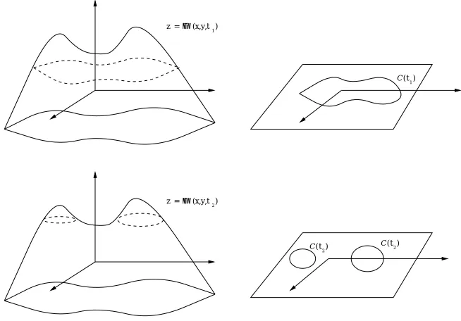
corre-sponding to the curve’s rest position. In Figure 2.1, it can be observed that the level set formulation,

(27)

advan-tageous in handling topological changes when compared to parametric evolution methods of curves

(also called marker particle methods [126]). This is due to the fact that the zero level set ofneed

not be simply connected, may split, and merge during the evolution.

z = Φ

Φ

z = (x,y,t

2)

(x,y,t1)

t

t t

1

2 2

(

( (

)

) )

C

C C

Figure 2.1: Depiction of a level set formulation versus a parametric formulation of a curve. Left column: (Eulerian framework) Evolution of a level set function(x;y;t)as a graph on a fixed grid is shown at time

instantst 1and

t

2. Note that topology changes are handled naturally; Right column: (Lagrangian framework)

Evolution of zero level set values of the surface via marker particle methods, i.e. evolution of position vector of a curve,(X(p);Y(p))=C(p)is also shown at time instantst

1and t

2. Notice that it is hard to manipulate

topology changes, and serious bookkeeping is required.

The level set function is usually picked as the signed distance function from the zero level

curve which is the contour that is to be evolved. A fast level set method so called as narrowband

technique [2] developed for propagating interfaces is used in the implementation. To speed up

the curve evolution algorithms we develop in this thesis, a periodical re-initialization of the signed

distance function, i.e. the level set function, is also carried out by the technique developed by [152].

In the level set equation, (2.19), the speed functionF may be given byF =+, with an

advection (first term on the right), and a diffusion term or a curvature term (second term on the

right). With a simplest flow whenF =1,

t

= jjrjj; (2.22)

(28)

singularities, i.e. points that are not differentiable, in finite time [126]. Once such points develop,

the normal is not defined at those points, and the propagation becomes ambiguous. Thus, in order

to continue the evolution, a weak solution is required. Note that a solution is a weak solution of a

differential equation if it satisfies an integral formulation of the equation. This in turn implies that

the weak solution, as a potential solution, may not require the same degree of differentiability, and

allows for more general solutions [126]. A way to obtain such a solution is provided by Sethian,

through the notion of an entropy condition, also called Huygen’s construction. This is motivated by

an analogy of a curve with a propagating flame, and once a point is ignited by the expanding flame

(curve), it stays burnt. That is, information once lost, can not be re-created during the evolution. The

parallelism of this development and the theory of viscosity solutions of Hamilton-Jacobi equations,

as well as shocks and rarefaction fans formations in hyperbolic conservation laws can be found

in [126]. To solve the Eq.(2.22), stable numerical schemes are developed, which select the correct

weak solution corresponding to the viscous limits of the associated curvature-driven equations. See

[86, 88] for detailed discussions on hyperbolic conservation laws. Upwind differencing schemes in

computing first order spatial derivatives which use values upwind of the direction of information

propagation, are widely employed [126]. The curve evolution equations we develop in this thesis

are curvature-driven equations, for which central-differencing schemes for the spatial derivatives

and forward-differencing schemes for the time derivatives are adequate. For the implementation of

the level set method, and its re-initialization step, however, upwind differencing schemes are used.

2.3 Overview of Segmentation Methods

The problem of image segmentation refers to the partitioning of a domainof a given imageI into

regions such that each region has properties distinct in some sense. It is expected that the resulting

partitions correspond to meaningful parts of objects in an image. Image segmentation is an essential

first step in early vision and provides a mechanism for an automatic analysis of image contents.

Some important applications include automatic target recognition, remote sensing, automatic visual

inspection in manufacturing processes, biomedical image analysis, tracking objects in motion, and

so on. In the context of remote sensing of the earth for instance, the image would be partitioned into

regions of different terrain or land type.

An initial task for segmentation is to determine the features which delineate and reliably

(29)

intensity, color, and texture. Following the definition of features for the segmentation problem, it

is necessary to select a “good” criterion for capturing and evaluating the features which yield a

partition of the image domain into “different” regions.

Existing image segmentation methods may broadly be classified into four groups [153] as

de-scribed in the next subsections.

2.3.1 Thresholding and Local filtering approaches

Perhaps the earliest approaches to image segmentation are based on thresholding techniques. They

rely on a very simple concept which is to compare each pixel value (I(x;y);(x;y) 2 ) with a

parameter (threshold) and decide whether the pixel is within the region or not. The value of the

threshold may be globally or locally set [112, 134]. In most methods, the threshold is chosen from

the intensity histogram of either the whole image or local regions of the image.

Local filtering approaches for image segmentation are based on detection of edges which

cor-respond to object boundaries or the boundaries between image regions. The celebrated early work

by Marr [96] and based on a “primal sketch” concept entailed localizing edges in the image for

subsequent use by high level image processing steps. Marr and Hildredth [97] developed an edge

detection filter based on local maxima of the gradient magnitude. When the first derivative achieves

a maximum, the second derivative is zero. For this reason, an edge detection strategy is to isolate

zeros of the second derivatives ofI. The differential operator used in these so-called zero-crossing

edge detectors, is the Laplacian. In order to mitigate the increase in pixel noise due to

differenti-ation, the image is pre-filtered with a lowpass filter such as a Gaussian kernel. A variant of this

idea such as the Canny edge detector [22] uses the zero-crossings of the second order operator in

Eq.(2.6) instead of the Laplacian. For efficient implementations, Deriche in [40], derives exact

recursive filters, taking a similar analytical approach to Canny.

Segmentation techniques in this group make use of local information, and can often be

imple-mented as a convolution of the given image with the impulse response of a local filter for efficiency

sake. They, however, rely on high gradient values in the image to detect prominent boundaries

between regions, hence, making them sensitive to noise and affecting the continuity of the edge

(30)

2.3.2 Region growing techniques

Region growing techniques partition an image domain into k disjoint regions O 1

;;O k, (i.e.,

= S k i=1 O i

), such that the image I o

is homogeneous in some sense within each region. Each

regionO

iis a connected region. Morel and Solimini [100] describe a general multiscale approach

to region growing as follows: (i) Initialize the algorithm with the finest possible segmentation at

a small scalet, i.e. consider each pixel as a separate region; (ii) Merge all pairs of regions whose

“merging” improves the segmentation; (iii) Iterate (go to (ii)) by increasing the scale parameter.

Choosing the criterion to perform step (ii) results in different algorithms.

For instance, a piecewise (p-w) constant model for the image is used by [78] as the merging

criterion. To a regionO

i, the average value of I

o

over that region is assigned. Given average values

I

i in region O

i and I

j in a neighbor region O

j, the regions O

i and O

j are merged by removing

the boundary between them and replacing bothI i and

I

j with their weighted average jO i jI i +jO j jI j jOij+jOjj . HerejO i

jis the area of regionO

i. The algorithm looks for a decrease of global energy by merging

these regions and by updating the image toI. The global energy is a least squares criterion, i.e.

R

jjI I

o jj

2

plus a penalty on the total length of the boundaries`. However, the quadratic penalty

on the difference between the estimateI and the initial dataI o

is not well suited to non-Gaussian

noise, such as speckle noise in SAR images.

An earlier method by Pavlidis in [100] also starts by taking all pixels as regions, and merging

every pair of regionsO iand

O

j such that variance of I o overO i S O

j is less than

t(scale).

Variants of region growing or merging methods may yield alternative approaches, e.g. region

splitting, and region split-and-merge methods ( [100]) which combines the two.

Region growing methods have an advantage of using statistics inside regions, they, however,

often generate irregular boundaries [153].

2.3.3 Active contour methods

Active contour models have been widely used in image segmentation applications. The general idea

in an active contour framework is to define energy functionals whose local minima comprise a set

(31)

Snakes

One of the pioneering works in this field is due to Kass, Witkin, and Terzopoulos [70] who addressed

the problem of finding salient image contours like boundaries of objects, edges, lines, by so-called

“snakes” algorithms. They aimed at having the snake lock onto image features by minimizing an

integral measure which represents the snake’s total energy. By adding suitable energy terms to the

minimization, it is possible for a user to push the model out of a local minimum towards the desired

solution. Initially, the user places some contour (snake) near an image structure. The constraint

forces that act on a snake then push the snake towards features of interest.

Representing the position of the contour parametrically, C(p) = (X(p);Y(p)), where p 2

[0;1], Kass et.al. defined the snake’s total energy functional, as

E(C(p))= Z

1

0

Eimage(C(p))dp+ Z

1

0

Eint(C(p))+Econ(C(p))dp: (2.23)

Here,Eintrepresents the internal energy of the snake due to bending:

Eint=(w 1

(p)jjC p

(p)jj 2

+w

2 (p)jjC

pp (p)jj

2 )=2;

where w 1 and

w

2 control the “tension” and “rigidity” of the snake respectively. (Note that the

subscripts denote derivatives with respect to p, and jjjj denotes the standard Euclidean norm.)

Their basic snake model is a spline under the influence of image forces, internal constraints, and

other general constraint forces, Econ. In an image force, R

1 0

Eimage(C(p))dp, Eimage(x;y) is a

scalar potential field defined on the image plane. The local minima of

R

Eimage attract the snake.

For example,Eimage can be chosen as an edge functionalEedge = jjrI(x;y)jj 2

, which drives the

snake to contours with large image gradients, i.e. the intensity edges.

First Connection between Curve Evolutions and Active Contours

The mathematical foundation of another class of geometric active contours was based on Euclidean

curve shortening. Defining the length functional (see arclength definition (2.9))

L(t)= Z

1

0

@C(t)

@p

(32)

then differentiating (taking the “first variation”), and using integration by parts, we have L 0 (t)= Z L(t) 0 @C @t ;N ds

whereis the curvature,N is the inward unit normal, andjj @C

@p

jjdp= ds. Thus the direction in

whichL(t)is decreasing most rapidly is achieved when

@C

@t

=N

which defines a gradient flow. (For the derivation of this curve length shortening flow, see [148].)

A new active contour paradigm was proposed in [25, 72, 148], by changing this ordinary Euclidean

arc-length function along a curveC(p)with parameterpgiven by

ds=jjC p

jjdp=(X 2 p +Y 2 p ) 1=2 dp to ds

=ds=(X

2 p +Y 2 p ) 1=2 dp

where(x;y)is a positive differentiable function. Thus a new metric is defined with which a new

gradient flow is to be found. The gradient flow for the curve shortening relative to the new metric

ds

will be computed, then the first variation of

L (t)= Z 1 0 @C @p dp;

will lead to

@C

@t

=( rN)N:

The metricds

has the property that it becomes small where

is small and vice versa. Thus at such

points, lengths decrease, and less energy is needed in order to move. If one wants the contour lock

onto edges of an image, then it is reasonable to construct a weight which is almost zero near edges,

and almost 1 when it is far from the edges. SincejjrIjjis a local indicator of strength of edges in

an image,is chosen as

=

1

1+jjrIjj :

(33)

Ω\ R Rf

v

C

u R

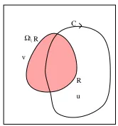
Figure 2.2: A piece-wise constant image consisting of two regions.

The initial contour has hence to be reasonably close to boundaries. The local property also causes

these models to be very sensitive to noise.

Region-based Active Contours

Region-based active contours were proposed to overcome the problems with the geometric or

geodesic [25, 72, 148] active contours by using both local and global information. The main idea is

to assume that the image consists of a finite number of regions, that are characterized by a

prede-termined set of features or statistics such as means, variances, textures etc. These features/statistics

can be estimated from the image data, hence an energy functional may be constructed to pull these

statistics apart, i.e. maximize the distance between them in order to separate the corresponding

regions. One advantage over the models in the previous subsection is that there is no need to

cal-culate gradients of the image which are usually very sensitive to noise. Region based flows are

therefore much more robust to noise, at a cost of additional imposed assumptions on the images,

and additional computations.

One such assumption is one’s ability to approximate an image by constants, i.e. assuming that

the image consists of piecewise constant regions. Let an image consist of only two regions, a

foregroundR

f, and a background nR

f, and let these be approximated by constants. Fix C, an

arbitrary closed curve in the image domain, and thereforeis partitioned intoRandR c

, regions

inside and outsideC respectively (Figure 2.2). An energy functional to separate the means of the

two regionsRandR c

, sayuandvrespectively, is given by Yezzi, Tsai, and Willsky [149]

EYTW(C)= 1

2

(u v)

2

: (2.24)

A gradient-descent flow on the above energy functional will maximize the Euclidean distance

be-tween the mean of region R and the mean of region nR. The energy in (2.24) hence will be

(34)

the background.

A similar energy functional is given by Chan and Vese [29]

ECV(C)=

Z Z

R

(I u)

2

dxdy+

Z Z

nR

(I v)

2

dxdy: (2.25)

The resulting flow in the direction of the gradient descent will automatically move the contour

towards the boundary @R

f of the target shape, to minimize this fitting energy. For instance, an

initial contour encompassing the regionR

f will flow inward towards the boundary; while a contour

insideR

f will flow outward; and a contour which overlaps R

f will flow in both directions towards

the boundary. This makes the initial placement of the contour less restrictive.

The data term, resulting from this formulation, was, however, shown to possibly require

addi-tional regularization depending on the particular types of noise, e.g. for salt and pepper type noise,

the contour may weave around noisy regions and result in erroneous regions. A regularizing term

(penalty on the length of the curve) is added to yield for instance the following energy functional

E(C)=EYTW+ I

C

ds (2.26)

where

H

C

dsis the total arclength of the curve, andis a parameter which determines the amount

of the desired regularization. The aim is to thus prevent the length of the curve from getting

imprac-tically long and producing smooth boundaries. The corresponding gradient descent flow forEYTW,

can be shown to be

@C

@t

= (u v)(

I u

R

R dxdy

+

I v

R

nR dxdy

)N N;

= f

I

N N: (2.27)

(A very similar derivation for the first term (data term) is deferred to Chapter 4). The regularizing

term (second term above) may also be viewed as a shape prior which is especially very strong at

contour points with high curvature. Therefore, there is a trade-off between the data-driven term and

the regularizing term. The data-driven term, however, usually dominates the flow.

2.3.4 Global optimization approaches based on energy functionals

The goal of most active contour algorithms is to extract the boundaries of homogeneous regions

(35)

within homogeneous regions but not across the boundaries of such regions. A well-known

math-ematical model proposed by Mumford and Shah [102] simultaneously addresses both goals. They

develop an energy functional which approximates an image by smooth functions in each region

instead of constant ones. The Mumford-Shah (M-S) functional is given by

E(C;f R

;f R

c) =

Z Z

R (f

R I)

2

dxdy+

Z Z

R c

(f R

c I)

2 dxdy

+

Z Z

R jjrf

R jj

2

dxdy+

Z Z

R c

jjrf R

c jj

2

dxdy+

I

C

ds; (2.28)

whereC is the closed, smooth segmenting curve,I is the observed image data, f

Ris the smooth

function inside the curve,f R

cis the smooth function outside the curve. Minimizing Eq. (2.28) then

corresponds to finding estimatesf Rand

f R

c in regions

RandR c

respectively.

The first two terms in the M-S functional are the data-fidelity terms (like the measurement/

observation model), the second two terms are the smoothness terms in the given regions (like a

prior model forf givenC). The last term is a prior model for C which penalizes its arc length.

The M-S functional, hence, captures the desired properties of segmentation and reconstruction by

piecewise smooth functions as opposed to p-w constant models in Eq.(2.24), and Eq.(2.25).

There are numerous other algorithms based on minimizing different criteria such as Minimum

Description Length (MDL) criteria [87], Bayesian criteria [17]. The problem of minimizing energy

functionals such as Eq.(2.28) or other energy functionals (MDL or Bayes criteria) is principally

computational (e.g. simulated annealing [51]). To overcome this difficulty, algorithms such as

(36)

Chapter 3

Stochastic Differential Equations and

Geometric Flows

In this chapter, we present a new class of curve evolution equations for smoothing of structures

along the known orientation of salient lines in curves and images while preserving their important

features. The contents of this chapter are outlined as follows. After an introduction in Section 3.1,

we briefly review and recap, as was described in Chapter 2.2, some theoretical concepts associated

with the curve shortening flow, including its connection to a nonlinear, directional diffusion

equa-tion in which image values diffuse locally only along the direcequa-tions of its edges in Secequa-tion 3.2. In

Section 3.3, we provide a stochastic equivalent equation which in turn unveils a new

shape/feature-driven flow described in detail in Section 3.4, which we also believe could offer a variety of

appli-cations outside the recognition and classification problems. We conclude with some illustrating and

substantiating examples in Section 3.5, and conclusions in Section 3.6.

3.1 Introduction

In recent years curve evolution has emerged as an important application of partial differential

equa-tions (PDE’s) in image processing, computer vision, and computer graphics. Curve evolution

tech-niques have been applied not only to individual curves, for applications such as edge-detection,

skeletonization, and shape analysis, but have also been considered for their simultaneous action on

the level sets of an image in a number of geometrically based anisotropic smoothing algorithms.

Osher and Sethian [111, 126] extended this latter perspective to the treatment of individual curves

(37)

and surface evolution on a fixed grid. These techniques have aided a number of researchers in

push-ing the application of curve evolution to new limits by providpush-ing a simple framework for treatpush-ing

certain types of singularities such as shocks and topological transitions [109, 111].

Much of the research in curve evolution theory has centered around the so called geometric heat

equation [54] in which a curve is evolved along the normal direction in proportion to its signed

curvature. This flow is well known for its smoothing properties [74–76] and the fact that it

cor-responds to the gradient evolution for arclength (thereby earning the name curve shortening flow).

Because curvature is a purely geometric quantity (invariant to rotation and translation),

curvature-based motion gives rise to a Euclidean invariant scale space [5, 6, 147], allowing one to trace

fea-tures in a curve from finer to coarser scales as the evolution proceeds. An affine invariant scale space

can be obtained from a related curvature flow which depends upon the cube root of the curvature

(see [5, 124, 125]).

When applied to the level sets of an image, these flows have a powerful denoising effect when

run for a short amount of time. If run for too long, however, even large scale features will be

de-stroyed. The reason stems from the fact that as the geometric heat flow shrinks any closed curve, the

curve becomes more and more circular (elliptical in the case of the affine flow) and will eventually

collapse into a single point [54]. It is therefore not always possible to preserve desired features in

the shapes of objects (corners for example) if too much evolution is required to remove a significant

level of noise. Furthermore, it is not well understood how these curvature-based filters are affected

by different noise distributions and when this sort of problem may occur.

To the best of our knowledge, and aside from [80, 81], nonlinear diffusion in the previous

litera-ture was discussed from a purely deterministic perspective. In this chapter, we provide a stochastic

formulation of the geometric heat equation and use the resulting insights to develop a new class of

curvature-based flows and anisotropic diffusion filters which preserve desired features in the shape

of an object. Under these new flows, evolving curves take the limiting form of a polygon (see [20]

for evolutions of polygons related to the geometric and affine geometric heat flows, and [144] for

evolutions of polygons globally through an electric field concept). The resulting diffusion models

may therefore be applied for much longer periods of time without distorting the shapes of polygonal

objects in the image, thereby mitigating the tradeoff between noise removal and shape distortion.

Polygonal structures are ubiquitous in images of man-made objects (buildings, roads, vehicles,

and so on), which contain many straight lines, often oriented in particular directions (e.g. horizontal

(38)

features is not only desirable when filtering an image which contains these types of shapes, but

is also important when applying low level smoothing to an extracted shape since such features

constitute important and powerful cues for recognizing objects in higher level vision algorithms.

We will present both applications in this chapter. From a dual perspective to our contour-based

approach to shape representation, skeletonization approaches may also allow shape analysis without

displacement of corners [18, 35, 75, 107, 118, 129].

In this chapter, we develop a new class of curve evolutions, which are obtained by a modification

of the geometric heat equation. Given an initial shape in the form of a continuous curve, the class of

curve evolution equations we will obtain, deform it into a pre-specified final polygonal shape. The

problem of deforming an input shape into a different form has been of interest in various fields such

as computer graphics [52].

3.2 Background

The geometric heat equation, introduced in Chapter 2, may be obtained as can be recalled in a

geometric manner by specifying the evolution of each level curve in the image. LetC denote a

particular iso-intensity contour which we will deform over time via the following flow,

C t

=C

ss

=N (3.1)

wheresdenotes the arclength parameter,the Euclidean curvature, andN the inward unit normal.

Equation (3.1), referred to as the Geometric Heat Equation (GHE), is well known for its smoothing

properties. It has been shown by Grayson [54] that any closed, embedded curve evolving according

to (3.1) will convexify and smoothly shrink to a single point in finite time, becoming more and more

circular along the way. If we apply the geometric heat flow to every single level curve in the image

we obtain the same anisotropic diffusion equation that we derived in Chapter 2. To see this, note

that at timeteach level curveC k

(where the indexkdistinguishes one level curve from another)

is implicitly described byu(t;x;y) =u k

whereu k

denotes a particular intensity in the image. Let

us choose a parameterization of C k

so that C k

(t;p) = (X(t;p);Y(t;p)) forp 2 [0;1]and for

allt 0. We may then write u t;C k

(t;p)

= u t;X(t;p);Y(t;p)

= u

k

. Differentiating this

expression with respect totyields

u t

+ruC

t =u

t

Curve and Polygon Evolution Techniques for Image Processing

Biography

Acknowledgments

Table of Contents

List of Figures

Chapter 1

Introduction

1.1

Thesis Motivations and Contributions

1.2

Thesis Summary and Organization

Chapter 2

Preliminaries

2.1

Notation

2.2

Image and Curve Evolution Techniques

2.3

Overview of Segmentation Methods

Chapter 3

Stochastic Differential Equations and

Geometric Flows

3.1

Introduction

3.2

Background