Development of a Moving Finite Element-Based Inverse Heat Conduction Method for Determination of Moving Surface Temperature

DEVELOPMENT OF A MOVING FINITE

ELEMENT-BASED INVERSE HEAT CONDUCTION METHOD FOR

DETERMINATION OF MOVING SURFACE

TEMPERATURE

A. H. Kakaee and B. Farhanieh

School of Mechanical Engineering, Sharif University of Technology Tehran-Iran, [email protected]

(Received: October 16, 2002 – Accepted in Revised Form: June 10. 2004)

Abstract A moving finite element-based inverse method for determining the temperature on a moving surface is developed. The moving mesh is generated employing the transfinite mapping technique. The proposed algorithms are used in the estimation of surface temperature on a moving boundary with high velocity in the burning process of a homogenous low thermal diffusivity solid fuel. The measurements obtained inside the solid media are used to circumvent problems associated with sensor and the receding surface. As the surface recedes, the sensors get swept over by the thermal penetration depth. The produced oscillations occurring in certain intervals in the solution is a phenomenon associated with this process. It is shown that the presented method can be used successfully for a wide range of thermal diffusivity coefficients.

Key Words Moving Finite Element, Control Volume-Finite Element, Inverse Heat Conduction Problem, Moving Boundary

ﻩﺪﻴﻜﭼ

ﻩﺪﻴﻜﭼ

ﻩﺪﻴﻜﭼ

ﻩﺪﻴﻜﭼ

ﻩﺪﺷﻪﺋﺍﺭﺍﻙﺮﺤﺘﻣﺢﻄﺳﻚﻳﻱﺎﻣﺩﻦﻴﻴﻌﺗﻱﺍﺮﺑﻙﺮﺤﺘﻣﺩﻭﺪﺤﻣﺀﺍﺰﺟﺍﻪﻳﺎﭘﺎﺑﺵﻭﺭﻚﻳﻪﻟﺎﻘﻣﻦﻳﺍﺭﺩ

ﺖﺳﺍ

. ﻭﻊﻳﺮﺳﻲﺷﻭﺭﻪﻛﺖﺳﺍﻩﺪﺷﻩﺩﺎﻔﺘﺳﺍﺖﻳﺎﻬﻧﻲﺑﺖﺷﺎﮕﻧﺵﻭﺭﺯﺍﺯﺎﻴﻧﺩﺭﻮﻣﻥﺎﻣﺯﺎﺳﻲﺑﻪﻜﺒﺷﺪﻴﻟﻮﺗﻱﺍﺮﺑ

ﺪﺷﺎﺑﻲﻣﺪﻣﺁﺭﺎﻛ

.

ﺑﻙﺮﺤﺘﻣﺯﺮﻣﻚﻳﺢﻄﺳﻱﺎﻣﺩﻦﻴﻤﺨﺗﻱﺍﺮﺑﻩﺪﺷﻪﺋﺍﺭﺍﻢﺘﻳﺭﻮﮕﻟﺍ

ﻦﺘﺧﻮﺳﺪﻨﻳﺍﺮﻓﺭﺩﻻﺎﺑﺖﻋﺮﺳﺎ

ﺖﺳﺍﻪﺘﻓﺮﮔﺭﺍﺮﻗﻩﺩﺎﻔﺘﺳﺍﺩﺭﻮﻣﻦﻴﻳﺎﭘﺫﻮﻔﻧﺐﻳﺮﺿﺎﺑﺪﻣﺎﺟﺖﺧﻮﺳﻚﻳ

.

ﻪﺑﻢﺴﺟﻞﺧﺍﺩﻩﺪﺷﻱﺮﻴﮔﻩﺯﺍﺪﻧﺍﻱﺎﻫﺎﻣﺩ

ﺭﺩﻪﻈﺤﻟ ﺮﻫ ﺭﺩﻡﺯﻻ ﺕﺎﻋﻼﻃﺍﻭﺪﻨﻛ ﻪﻠﺑﺎﻘﻣﺖﺧﻮﺳ ﻪﻬﺒﺟﻱﻭﺮﺸﻴﭘ ﻪﻠﺌﺴﻣ ﺎﺑﻪﻛ ﺪﻧﺍ ﻩﺪﺷﻪﺘﻓﺮﮔ ﺭﺎﻛﻪﺑ ﻲﻋﻮﻧ ﺪﺷﺎﺑ ﺭﺎﻴﺘﺧﺍ

.

ﻮﺳ ﻪﻬﺒﺟ ﻱﻭﺮﺸﻴﭘ ﺎﺑ ﻥﺎﻣﺰﻤﻫ

ﺩﺩﺮﮔ ﻦﻳﺰﮕﻳﺎﺟ ﻲﺒﺳﺎﻨﻣ ﻮﺤﻧ ﻪﺑ ﺕﺎﻋﻼﻃﺍ ﺎﺗ ﺖﺳﺍ ﻡﺯﻻ ﺖﺧ

.

ﻦﻳﺍ

ﻲﻣﺕﺎﻋﻼﻃﺍﻝﺎﺳﺭﺍﺭﺩﻝﻼﺘﺧﺍﺚﻋﺎﺑﻲﻨﻳﺰﮕﻳﺎﺟ ﺩﺎﺠﻳﺍﻝﻮﻤﻌﻣﻱﺎﻬﺘﻟﺎﺣﻪﺑﺖﺒﺴﻧﻪﻓﺎﺿﺍﺕﺎﻧﺎﺳﻮﻧﻪﺠﻴﺘﻧﺭﺩﻭﺩﺩﺮﮔ

ﻲﻣ ﺩﻮﺷ

.

ﻭﻪﺘﻓﺮﮔ ﺭﺍﺮﻗﻞﻣﺎﻛﻲﺳﺭﺮﺑﺩﺭﻮﻣﻱﺍ ﻪﻠﺌﺴﻣﻦﻴﻨﭼﺭﺩﻩﺪﺷﻪﺋﺍﺭﺍﻢﺘﻳﺭﻮﮕﻟﺍﺯﺍﻩﺩﺎﻔﺘﺳﺍﻪﺠﻴﺘﻧﻪﻟﺎﻘﻣﻦﻳﺍﺭﺩ

ﻞﻤﻋ ﺐﺳﺎﻨﻣ ﺭﻮﻃﻪﺑ ﻲﺗﺭﺍﺮﺣﺫﻮﻔﻧ ﺐﻳﺮﺿ ﺕﺍﺮﻴﻴﻐﺗ ﻊﻴﺳﻭﻩﺩﻭﺪﺤﻣ ﻚﻳ ﻱﺍﺮﺑ ﺵﻭﺭﻪﻛ ﺖﺳﺍ ﻩﺪﺷ ﻩﺩﺍﺩﻥﺎﺸﻧ ﻲﻣ ﺪﻨﻛ

.

1. INTRODUCTION

Direct temperature measurement on a moving surface, such as the flame temperature on a solid fuel or surface temperature of a melting material is a very difficult and expensive process. Two different approaches can be taken in obtaining information on surface heating. In the first approach, surface temperatures are measured directly. This approach is proven difficult due to extreme temperatures at the moving surface. The second approach, which bypasses direct surface measurements, is based on an indirect or inverse

temperature measurements taken within the medium, has numerous practical applications [1-8].

The utilization of inverse heat conduction analysis has received great attention during last decade. Various methods, including analytical or numerical approaches, have been developed to solve inverse heat conduction problems. There are two processes dealing with the inverse problems: the processes of analysis and the process of optimization. In the former one, the unknown quantities are assumed, and then the results of the problem are solved directly using the numerical methods. The conventional numerical methods are finite difference, finite volume, finite element, and boundary element methods. The solutions from the mentioned process are used to integrate with data measuring at the interior point of the solid. Consequently, a nonlinear problem is established for the process of optimization. In this process, an optimizer such as sensitivity analysis, the conjugate gradient method, the regularization method, and so on, ought to be used to guide the exploring points systematically to search for a new set of guess quantities, which is then substituted for the unknown quantities in analysis process. However, the constraints arising when dealing with a moving boundary should be addressed with care.

Several studies of moving boundary related problem have been presented in the past. Huang et al. used conjugate gradient method for determining unknown conductance during metal casting in one-dimensional field [9]. Keanini and Desai employed inverse finite element reduced mesh method in order to predict multi-dimensional phase change boundaries [10]. The thermal diffusivity of this problem was around

s / m 10

1_× −7 2 _{and the work piece traveled at a} speed of 1.24_×10−4m/s_{. Woodbury and Ke} investigated a one–dimensional boundary inverse heat conduction problem with phase change to moisture bearing porous medium [11]. Xu and Naterer used inverse method to study the heat and entropy transport in solidification processing of material [12]. The thermal diffusivity of the materials was approximately in the order of

s / m

10−5 2 _{. The interface velocity was around}

s / m 10 6 .

7 _× −5 _.

This paper presents a unified moving finite element algorithm for the solution of general two-dimensional non-linear inverse heat conduction problem with moving boundary condition. The employed moving finite element method uses finite volume formulation [13] and keeps the numerical boundary consistent with the moving surface. The derived algorithm is capable of evaluating surface heat flux, surface temperature, and heat transfer coefficient on the moving surface. The mathematical framework of this method is so general that a variety of inverse heat conduction problems with moving boundary conditions and complex geometries can be treated. Other inherent complexities such as material non-linearity and the number and locations of the data points have all been included in the algorithm.

A numerical test case is presented to demonstrate the application of the algorithm. This application relates to the determination of the temperature on a moving surface of an annular homogenous solid fuel. The resulting temperature distribution can be used to assess the thermal behavior of the solid, as well as determination of the flame temperature.

2.THE DIRECT PROBLEM

The governing equation for a three dimensional, nonlinear, direct and unsteady heat conduction problem reads:

(

k

T

)

t

T

c

_p

=

∇

∇

∂

∂

.

ρ

(1)

where T denotes the temperature field and is the function of space and time. _ρ ,

c

_p, and k are density, specific heat capacity, and conductivity, respectively. In order to illustrate the implications of different types of boundary conditions in the formulation of the inverse problem, three different boundary conditions are considered:

( )

r

t

f

T

h

n

T

k

+

=

r

,

∂

∂

r

∈

Γ

,

t

>

₀

c

( )

r

t

q

n

T

k

=

b

r

,

∂

∂

−

r

r

∈

Γ

_q

,

t

>

0

(2-b)

( )

r

t

T

T

=

b

r

,

r

∈

Γ

,

t

>

₀

T

r

_(2-c)

The initial condition for Equation 1 is:

( )

r

T

T

=

₀

r

r

r

∈

Ω

,

t

=

0

(2-d)

where

Γ

_c

,

Γ

_q, and

Γ

_T are continuous boundary surfaces of the region _Ω.

h

,

f

,

q

b

,

T

b and

T

₀are known functions in the direct problem.

3. THE INVERSE PROBLEM

In the presented inverse heat conduction problem, one of the boundary conditions is unknown. Let assume that there are M temperature sensors in the region Ω where the measured temperatures are:

(

r

t

)

T

T

m _m

m

=

r

,

(3)

where

r

r

_mis the location vector of mth sensor. The measured data constitute a vector at time

t

:

[

_m

]

T

M m

m

m

T

T

T

T

r

=

_{1 2}

L

(4)

Superscript T is the transpose symbol. In order to explain the methodology used in this work, the boundary condition expressed in Equation 2-c is considered as the unknown boundary condition. However, the presented method is general and can be used for other types of boundary conditions too.

Assume that

T

bis a known variable. The temperature of the mth _{measuring point at location,}

m

r

r

is computed by solving Equation 1 and using the Galerkin interpolation method:

( )

r

t

T

T

c c _m

m

=

r

,

(4)

where superscript c stands for computed. Thus the

computed temperature vector at time

t

is:

[

_c

]

T

M c

c

c

T

T

T

T

r

=

_{1 2}

L

(5)

The inverse heat conduction problem is an ill condition problem and the computed temperatures

c

T

r

deviate from the measured temperatures

T

r

m due to the measurement errors [3]. Therefore, the solution of the problem is now defined as the least square solution of the errors:

(

T

c

T

m

) (

T

T

c

T

m

)

E

=

r

−

r

W

r

−

r

(6)

where W is the weighting matrix and by Beck’s assumptions, it can be calculated as follow [14]:

I

W

=σ

−2 ₍₇₎

σ is the variance of the measurement errors. As seen from Equations 1 and 2, E is the function of the temperature on the boundary,

T

b_{. In order to} minimize E, the partial derivative with respect to

b

T

must be equal to zero:

(

−

)

=

0









∂

∂

=

∂

∂

c m

T

b c

b

T

T

T

T

T

E

r

r

r

W

(8)

c

T

r

is also a function of

T

b_{. Using the Taylor} expansion series the following expression is obtained:

b b c

T c T T

c

T

T

T

T

T

_{b b b}

∆

∂

∂

+

=

∆ +

r

r

r

(9)

Substituting expression (9) in Equation 8 reads

(

c m

)

T b T

W

T

−

T

=

X

X

∆

T

X

r

r

(10)

where _b

c

T

T

∂

∂

=

r

X

is known as the sensitivity matrix. For the sake of simplicity the subscripts in Equation 10 are dropped.

Beck [1]:

(

)

(

) ( )

b n b n c m b n c m mn

T

T

T

T

T

X

ε

ε

−

+

=

1

N

n

M

m

=

1

,

2

,

K

,

and

=

1

,

2

,

K

,

(11)

where

ε

is a small positive number. b n

T

is defined as:

( )

r

t

T

T

b b

n

=

r

,

r

r

∈

Λ

n

,

n

=

1

,

2

,

K

,

N

(12)

where _T

N

n

n

=

Γ

Λ

=

U

₁ and

Λ

_i

I

Λ

_j

=

Φ

.

4. MOVING BOUNDARY FINITE ELEMENT METHOD

Moving boundary-moving mesh entails the use of a system whereby numerical boundaries are kept consistently on moving boundaries; the overall mesh configuration is continuously adjusted in the course of time to conform to any movement of the boundary. The finite element formulation is obtained by applying the Galerkin method to Equation 1, using the linear triangular elements witch is represent by Albert and O'Neil in 1986 [15]:

(

)

( )

0 d t , r N T . V c t T c T k . j p p = Ω           ∇ ρ − ∂ ∂ ρ − ∇ ∇

∫

Ω r r

J

j

=

1

,

2

,

K

,

(13)

where

N

_j

( )

r

r

,

t

is the basis function, and

V

r

is the mesh velocity. Note that this formulation has added a convection term to the governing numerical equation. This apparent convection is due to the movement of the mesh and highlights the fact that the problem is being analyzed through a coordinate system implicitly attached to the mesh. Albert and O'Neil [15] are used

the Standard Galerkin method. It is known that Standard Galerkin Method solution of convection–conduction equation of heat transfer leads to unstable results in high Peclet number cores. The accepted and widely use technique to cope with such problems is to use upwinding technique. It is used the first order upwind in finite element form, which is known as Petrov Galerkin method [16].

After descritization with linear triangular element and some rearrangement of formulation, Equation 13 can be rewritten in the form of finite volume formulation [17,18]:

0

.

_, 1 , 1 , ,

+

=

∂

∂

∑

∑

=

= i j

I i j i I i j i j

i

H

n

t

T

C

j j

r

r

(14)

where

I

_j is the number of nodes neighboring the jth _node.

j i

C

_, is a constant in each control volume. The second term in Equation 14 represents the summation of the fluxes across the faces of the jth node's control volume. For this formulation the Delauny control volume is used [17]. The Crank-Nicolson schemed is used to solve the ordinary differential Equation 14 at each time step [19]:

0 n . H 2 1 n . H 2 1 t T T C n j , i I 1 i i,j

1 n j , i I 1 i i,j I 1 i n j , i 1 n j , i j , i j j j =         +         + ∆ −

∑

∑

∑

= + = = + r r r r (15) where the superscript n denotes the time step. The

Equation 15 can be rewritten in the following compact form:

b

T

r

=

r

A

(16)

A is the coefficient matrix and

b

r

is called the force vector.

T

r

represents the temperatures at the nodes in region _Ω at time step (n+1).

coefficient matrix could become non-positive definite. Thus, the lower upper decomposition (LU) method is used for solving this system of linear equations [20]. Due to the large dimension of the coefficient matrix, the sparse matrix data structure is adopted for data storage [21].

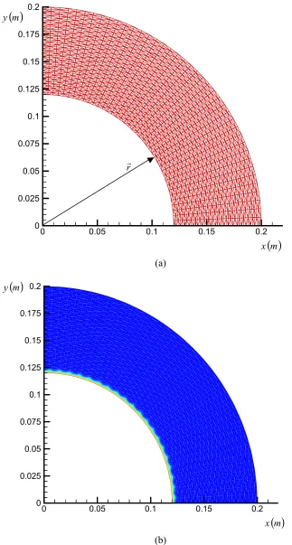
Owing to the complexity of the domain and the moving nature of the boundary, in order to minimize the CPU time the efficient algorithm of the transfinite mapping is used. Since the moving boundary may travel large distances and undergo a significant change in shape in the course of the solution, a flexible system for arranging the interior nodes must be applied in order to keep the mesh in a reasonable condition. The method used in this work to accomplish this task involves the generation of a new mesh each time step, using transfinite mappings.

Haber et al. [22], Gordon [23,24], and Hall [25] describe the transfinite mapping in terms of projectors. The transfinite mappings used in this work is the bilinear projector which is given by

( ) ( ) ( )

( ) ( ) ( )

( ) ( )( ) ( ) ( ) ( )

( ) ( ) ( )

1,1 s1 t F1,0

F st 1 , 0 F t 1 s 0 , 0 F t 1 1 s t s t s 1 s t s t 1 t , s P 2 1 2 1 − + − − + − − + ψ + ψ − + ξ + ξ − =

1

0

,

1

0

<

t

<

<

s

<

(17) This projector represents a continuous mapping of

a unit square in the transformed

( )

s

,

t

space onto the region to be meshed in the original

( )

x

,

y

F-space. In F-space the region has four sides described by the curves

ξ

₁

( )

s

,

ξ

₂

( )

s

,

ψ

₁

( )

t

and

( )

t

2

ψ

and four corners with coordinates

F

( )

s

,

t

where

s

and

t

equal zero or one. This projector maps equal divisions of the unit square in

( )

s

,

t

onto a desired shape as shown in Figure 1(a). In practice, a finite number of nodes are identified on each side: these correspond to discrete values of

ξ

and

ψ

. Thus

ξ

and

ψ

need not be smooth functions or any known functions at all. One only needs to specify nodal coordinates at various points along the boundary curves, such that these points may be identified with values of s and t between zero and one along opposing sides. In

principle, the use of higher order elements to treat more general topologies than are dealt with here can also be accommodated. The method will match any set of boundary curves exactly at all points on those curves if the actual boundary functions

( )

ξ

,

ψ

are used in Equation 17.

4. THE SOLUTION ALGORITHM

The sequence of the solution algorithm can be stated as:

1. Guess the boundary condition,

T

r

b. 2. Solve Equation 1 for

T

r

c.

3. Calculate the sensitivity matrix.

4. Solve the Equation 10 for

∆

T

band correct

b

T

r

.

5. Using the newly calculated

T

r

b solve Equation 14 for

T

r

c_.

6. Check the following convergence criteria:

1

ε

<

k

E

(18-a)

2

1

−

/

<

ε

+ k k

k

E

E

E

(18-b)

3

ε

<

∆

T

b _(18-c)

7. where superscript k denotes the iteration number.

ε

₁,

ε

₂and

ε

₃are arbitrary constants and their values are determined upon the accuracy requirement and cannot be smaller than the measuring error [26].

8. If none of these criteria is satisfied return to step three. Otherwise, the convergence in the solution is achieved.

5. RESULTS AND DISCUSSION

Based on the described method a computer code,

This code consists of transfinite mapping; mesh generator, moving finite element solver for direct problem, and LU decomposition solver with sparse matrix data structure for solving the linear system of equations.

The performance of the method is assessed by comparing the computed results of the inverse analysis with the simulated results based on the method presented by Ozisik [27]. In this method, the simulated temperature measurement

T

_mm is generated from the exact temperature in the problem and it is presumed to have measurement errors.

In other words, the random errors of measurement are added to the exact temperature. It can be shown in following equation:

σ

ω

+

=

m

exact m

m

T

T

m

=

1

,

2

,

K

,

M

(19)

where

T

_exactm denotes the exact temperature from the solution of the direct problem at the measuring location,

r

r

_m. _σ is the standard deviation of measurement errors, and _ω is a random variable with normal distribution with zero mean and standard deviation of 1.

For normally distributed random errors, the probability of a random value _ω lying in the range,

576 . 2 576

.

2 < <

−

ω

is 99%. The value of _ω is calculated by Gasdev subroutine [28].

5. TEST CASE

A critical case of a homogenous burning annular solid fuel is considered in the present work. Due to the burning process of the fuel, the inner surface recedes by a velocity of 10 mm/s. For the simplicity of the analysis, only one quarter of the circle is considered. The boundary and initial conditions of the case to be studied are given below:

K

T

=

1000

t

>

0

,

r

=

0

.

1

m

,

0

<

θ

<

90

°

(20-a)

K

T

=

300

t

>

0

,

r

=

0

.

2

m

,

0

<

θ

<

90

°

(20-b)

The physical properties of a typical solid fuel are [29]:

k

=

0

.

418

W

/

m

°

K

,

ρ

=

1750

kg

/

m

3_{, and}

K

kg

J

c

_p

=

1260

/

°

.

To apply the inverse heat conduction methodology to the moving boundary, the temperature of the inner surface is now considered unknown. The inverse analysis is performed by arranging nine thermocouples radially in the centerline of the domain 10 mm apart from each other.

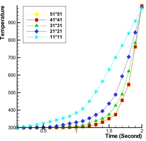
A typical grid is shown in Figure 1(a). The temperature contours at t = 2 seconds are plotted and presented in Figure 1(b). In order to investigate the grid size effect, exploratory test runs were performed under various grid sizes to compute the temperature at the third sensor. The temperature history for these grids is plotted in Figure 2. The maximum changes in the temperature between the coarsest mesh

11

11

×

and the finest mesh 51×51 are within 85%. The results show that by increasing the fitness of the grid to more than

41

×

41

no significant changes appear in the temperature history. The final computations were performed with

41

×

41

grid points to maintain relatively mo d e r a t e c o mp u t i n g t i me s i n t h e f i n a l calculations.

As seen in Figure 1(b), the thermal penetration depth of the heat flux is less than 3 mm. This is due to the effect of low thermal diffusivity of the solid fuel (less than

s

m

/

10

2

×

−7 2 _{). It is worth to mention that in a}

semi-infinite flat plate with no moving boundary and with the same physical properties as the test case, the temperature at the depth of 3 mm varies only by a degree centigrade after 2 seconds. In this problem, the effective mechanism of the heat flux penetration is the velocity of the surface. Thus, the sensitivity of the computational domain is very low to the variation of the surface temperature.

0 0.05 0.1 0.15 0.2

x

0 0.025 0.05 0.075 0.1 0.125 0.15 0.175 0.2

y

rr

( )

m x

( )

m y

(a)

0 0.05 0.1 0.15 0.2

x

0 0.025 0.05 0.075 0.1 0.125 0.15 0.175 0.2

y

( )

m x

( )

m y

(b)

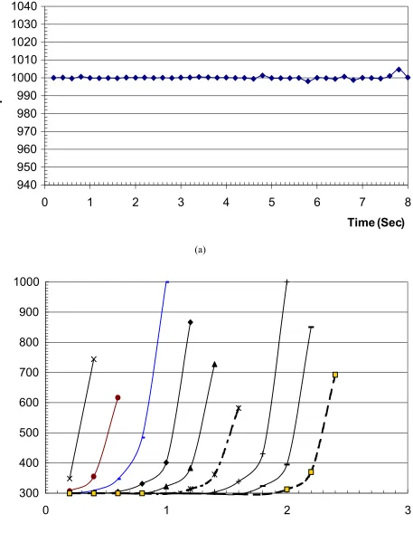
To investigate the influence of the thermocouple's errors on the solution, the variance of the difference between the simulated and the computed temperature of the moving surface,

σ

b

=

var(

T

b,c

−

T

b,s

)

1/2_{, is obtained and}

plotted for different

σ

m_{, in Figure 4. The variance} is obtained over the period of 8 seconds in Figure 4. As seen from this figure, the calculated variance increases with increasing

σ

m_{. This is an obvious} nature of the inverse heat conduction problem, increased errors in thermocouples readings increases the errors in computing boundary temperature values. This figure shows that the method is applicable for moving boundary problems. For example if K-type thermocouples, which have one degree centigrade normal error, are used, the error occurring in the solution will be approximately 1 degree centigrade according to Figure 4.

The influence of the thermal diffusivity,

α

on the solution is investigated by examining the variation

of

σ

b_{for different}

α

_{, assuming constant}

C

m

=

₀

.

1

°

σ

. The results are calculated over two different periods and presented in Figure 5. As seen from the figure, at low thermal diffusivity the variation of _σb _{is insignificant. However, at}

s / m 10−5 2 =

α a sharp decrease in _σb_{is observed.}

The sharp decrease in _σb _{is due to the fact that the}

thermal penetration depth is directly related to the thermal diffusivity. As _αincreases, the thermal penetration depth becomes larger, increasing the sensitivity of the adjacent thermocouple to the temperature of the moving surface. Increasing the value of

α

to more than

10

−4

m

2

/

s

_{, decreases} the errors in the solution.

6. CONCLUSION

A flexible hybrid method is presented for solving

0.5 1 1.5 2

Time (Second)

300 400 500 600 700 800 900

T

e

m

p

er

at

u

re

51*51 41*41 31*31 21*21 11*11

940

950

960

970

980

990

1000

1010

1020

1030

1040

0

1

2

3

4

5

6

7

8

Time (Sec)

Temperature

(a)

300

400

500

600

700

800

900

1000

0

1

2

3

inverse heat conduction problem with moving boundary. Based on the moving finite element and transfinite mapping properties, the method is developed for the cases with complex moving boundary conditions. The unique feature of the proposed algorithm is that the method can be used to treat any cases with unknown surface heat flux, surface temperature, and heat transfer coefficient on the moving surface. The applicability of the proposed method has been demonstrated in a case involving the burning of a homogenous solid fuel with unknown surface temperature on the receding boundary. The excellent correlation of the computed temperature histories and those measured at selected locations in the solid wall provides a clear indication of the credibility of the proposed method. From the results, it appears that reasonably accurate estimation could be made even when measurement errors are considered. The velocity of the receding surface on the formation of the thermal penetration depth and hence on the sensitivity of the sensors measuring the

temperature is recognized and discussed. Some oscillations in temperature readings are observed when a sensor is swept over by the thermal penetration depth and left the computational domain. Thus in online measurements of the boundary temperature, these oscillations should be omitted from the results. The variation of the thermal diffusivity on the solution is also considered.

7. REFERENCES

1. Beck, J. V., Blackwell, B. and Clair, C. R. ST., Jr., “Inverse Heat Conduction”, John Wiley and Sons, (1985). 2. Hensel, E., “Inverse Theory and Applications for

Engineering”, Prentice Hall, (1991).

3. Engl, H. W., Hanke, M., Neubauer, A., “Regularization of Inverse Problems”, Kluwer Academic Pub., (1996). 4. Isakov, V., “Inverse Problems for Partial Differential

Equations”, Springer- Verlag New York, Inc., (1998). 5. Ozisik, M. N., Orlande, H. R. B., “Inverse Heat Transfer:

Fundamentals and Application”, Taylor and Francis,

1.E-07

1.E-06

1.E-05

1.E-04

1.E-03

1.E-02

1.E-01

1.E+00

1.E+01

1.E-08 1.E-07 1.E-06 1.E-05 1.E-04 1.E-03 1.E-02 1.E-01 1.E+0

0

( )

C

m

°

σ

( )

C

b

°

σ

2000.

6. Kakaee, A. H.and Farhanieh, B., “Comparison of Regularization Methods for Inverse Heat Conduction Problems”, International J. of Engineering Science, Iran University of Scince and Technology, Vol. 13, No. 4, (2002), 173-190.

7. Taler, J., Zima, W., “Solution of Inverse Heat Conduction Problems Using Control Volume Approach”, Int. J. Heat and Mass Transfer, Pergamon Press, Vol. 42, (1999), 1123-1140.

8. Keanini, R. G., Desai, N. N., “Inverse Finite Element Reduced Mesh Method for Predicting Multi Dimensional Phase Change Boundaries and Nonlinear Solid Phase Heat Transfer”, Int. J. Heat and Mass Transfer, Pergamon Press, Vol. 39, (1996), 1039-1049.

9. Huang, C. H., Ozisik, M. N., Sawaf, B., “Conjugate Gradient Method for Determining Unknown Conductance During Metal Casting”, Int. J. Heat Mass Transfer, Vol. 35, No. 7, (1992), 1779-1786.

10. Keanini, R. G., Desai, N. N., “Inverse Finite Element Reduced Mesh Method for Predicting Multi-Dimensional Phase Change Boundaries and Non-Linear Solid Phase Heat Transfer”, Int. J. Heat Mass Transfer, Vol. 39, No. 5, (1996), 1039- 1049.

11. Woodbury, K. A. and Ke, Q., “A Boundary Inverse Heat Conduction Problem with Phase Change for Moisture- Bearing Porous Medium”, Inverse Problem in Engineering: Theory and Practice: 3rd _{Int. Conference on}

Inverse Problems in Engineering, (June 13-18, 1999).

12. Xu, R. and Naterer, G. F., “Inverse Method with Heat and Entropy Transport in Solidification Processing of Materials”, J. Material Processing Technology, Vol. 112, (2000), 98-108.

13. Barth, T., ‘On Unstructured Grids and Solvers”, VonKarman Inst. Lect. Series in Comp. Fluid Dynamics, Vol. 3, (1990), 1-65.

14. Beck, J. V, “Non-Linear Estimation Applied to the Nonlinear Heat Conduction Problem”, Int. J. Heat Mass Transfer, Vol. 13, (1970), 703-716.

15. Albert, M. R., O'Neil, K., “Moving Boundary- Moving Mesh Analysis of Phase Change Using Finite Elements with Transfinite Mappings", Int. J. Numer. Meth. Engineering, Vol.23, (1986), 591-607.

16. Zienkiewicz, O. C., Taylor, R. L., “The Finite Element Method” 5th Ed., Vol. 3: Fluid Dynamics, McGraw Hill Book Co., (2000).

17. Barth, T., “On Unstructured Grids and Solvers", VonKarman Inst.Lect.Series in Comp. Fluid Dynamics, Vol. 3, (1990), 1-65.

18. Kakaee, A. H., “ Solution of the Two Dimensional Navier Stokes Equations on Unstructured Triangular Meshes for Laminar Incompressible Fluid Flow”, MSc Thesis, Sharif University of Technology, (1995).

19. Harrier, E. and Warner, G., “Solving Ordinary Differential Equations: Stiff Problems”, Springer Verlag, (1991).

20. Golub, G. H., Vanloon, C. F., “Matrix Computations”, John Hopkins Univ. Press, (1989).

1.E-07

1.E-06

1.E-05

1.E-04

1.E-03

1.E-02

1.E-01

1.E+00

1.E+01

1.E-08 1.E-07 1.E-06 1.E-05 1.E-04 1.E-03 1.E-02 1.E-01 1.E+0

0

( )

C

b

°

σ

( )

m

2

/

s

α

21. Duff, I. S., Erisman, A. M. and Reid, J. K., “Direct Methods for Sparse Matrices”, Clarendon Press, Oxford, (1986).

22. Haber, R., Shepard, M. S., Abel, J. F., Gallagher, R. H. and Greenberg, D. P., “A General Two Dimensional Graphical Finite Processor Utilizing Discrete Transfinite Mappings”, Int. J. Num. Meth. Engng., Vol. 17, (1981), 1015-1044.

23. Gordon, W. J., “Blending- Function Methods Bi-variate and Multivariate Interpolation and Approximation”,

SIAM, J. Numer. Anal., Vol. 8(1), (1971), 158-177. 24. Gordon, W. J., Hall, C. A., “Construction of Curvilinear

Coordinate Systems and Application and Approximation to Mesh Generation”, Int. J. Num. Meth. Engng., Vol. 7, (1973), 461-477.

25. Hall, C. A., “Transfinite Interpolation and Applications to

Engineering Problems, in Theory of Approximation”, Eds., Low and Sahney, Academic Press, (1976), 308-331. 26. Huang, C. H., Yan, J. Y., “An Inverse Problem in

Predicting Temperature Dependent Heat Capacity Per Unit Volume without Internal Measurements”, Int. J. Numer. Meth. Engineering, Vol. 39, (1996), 605-618. 27. Jarny, Y., Ozisik, M. N. and Bardon, J. P., “A General

Optimization Method Using Adjoint Equation for Solving Multidimensional Inverse Heat Conduction”, Int. J. Heat Mass Transfer, Vol. 34, (1991), 2911-2919.

28. Press, W. H., Teukolsky, S. A., Vetterling, W. T., Flannery, B. P., “Numerical Recipes in FORTRAN: Art of Scientific Computing”, Cambridge Univ. Press, (1992).