R E S E A R C H
Open Access
Regularization method for the radially
symmetric inverse heat conduction problem
I Djerrar, L Alem and L Chorfi
**Correspondence: l_chorfi@hotmail.com
Lab. LMA, Badji Mokhtar University, Annaba, Algeria
Abstract
We consider an axisymmetric inverse problem for the heat equation inside the cylindera≤r≤b. We wish to determine the surface temperature on the interior surface{r=a}from the Cauchy data on the exterior surface{r=b}. This problem is ill-posed. Using the Laplace transform, we solve the direct problem. Then the inverse problem is reduced to a Volterra integral equation of the first kind. A standard Tikhonov regularization method is applied to the approximation of this integral equation when the data is not exact. Some numerical examples are given to illustrate the stability of the proposed method.
MSC: 35K05; 65N06; 35R30; 44A10
Keywords: ill-posed problem; radially symmetric heat equation; Laplace transform; Tikhonov regularization
1 Introduction
The inverse heat conduction problems (IHCPs) have many applications in different branches of science and technology. It consists in determining the temperature and heat flux on both sides of the boundary when one side is inaccessible to measurements.
The mathematical model of our problem can be described by the axisymmetric heat equation
∂u ∂t(r,t) =
∂u ∂r(r,t) +
r
∂u
∂r(r,t), r∈(a,b),t> , ()
with the boundary conditions
u(b,t) =g(t), ∂u
∂r(b,t) =h(t), t≥, ()
and the initial condition
u(r, ) = , r∈(a,b), ()
whereris the radial coordinate, and <a<b.
Our purpose is to determine the boundary condition
u(a,t) =f(t), t≥. ()
from the measured Cauchy data (g,h). It is known that this problem is severely ill-posed in the sense that if the solution exists, then it does not depend continuously on the datag. Indeed, a small perturbation in the data may cause dramatically a large error in the solution u(·,t). Hence, a regularization method is needed.
The standard problem of the heat conduction in Cartesian coordinates ut =uxx,x∈
[, ],t> , with the datau(,t) =f(t) andux(,t) = is well studied by various methods.
The Fourier method was used in [–]. The mollification method and projection regular-ization based on the Laplace and Fourier transforms are applied respectively in [] and []. For axisymmetric problems, we should mention recent articles. In [, ], the authors consider an axisymmetric IHCP of determining the surface temperature from a fixed lo-cation inside a cylinder. In [, ], the authors investigated the case of identifying a source from the final data. Xiong [] studied the problem of identifying a boundary condition by the method of quasi-reversibility. A modified Tikhonov regularization method was ap-plied for an axisymmetric backward heat equation in []. Lesnic et al. [] apap-plied the method of fundamental solutions (MFS) (with a Tikhonov regularization) to the radially symmetric inverse heat conduction problem (IHCP) analogous to our problem. Inverse problems for fractional diffusion equations are studied by many authors; for example, we mention the recent article [].
In this paper, we formulate problem ()-() as an integral equation of the first-kind of Volterra type. Then we use the Tikhonov regularization method to approximate this equa-tion. To the author’s knowledge, there are no papers devoted to IHCP with radial axisym-metry using the Laplace transform. Our contribution can therefore be considered as a generalization of the paper [] to the axisymmetric case.
This paper is organized as follows. In Section , we give a representation of the solution of the direct problem using the Laplace transform. Then finite difference method (FDM) is applied to give numerical approximation. In Section , our inverse problem is reduced to the integral equation of Volterra type; then we apply the Tikhonov regularization method to compute the boundary temperatureu(a,t) =f(t) from the Cauchy datau(b,t) =g(t), ur(b,t) = and give some numerical results. Finally, in Section , we present a conclusion.
2 Direct problem
Problem ()-() can be reduced to an integral equation. For this, we assume thatu(a,t) = f(t) is known and (for simplicity) h(t) = . We consider the following direct problem: givenf, findu(x,t) such that
∂u ∂t(r,t) =
∂u ∂r(r,t) +
r
∂u
∂r(r,t), r∈(a,b),t> ,
u(a,t) =f(t), ∂u
∂r(b,t) = , t≥,
u(r, ) = , r∈(a,b).
()
We have the following uniqueness theorem.
Theorem Problem()has at most one solution in the space
Proof Letu(r,t) be a solution of the homogeneous problem () (withf = ). Multiplying PDE byruand integrating by parts over the interval (a,b), we obtain the identity
b a
∂u ∂tur dr+
b a
∂u ∂r
r dr= .
We setE(t) =abur dr,t≥, which leads to dE
dt = b
a
utur dr= –
b a
(ur)r dr≤,
and thereforeE(t) =E() = for allt≥, andu(r,t) = ,r∈(a,b),t≥.
2.1 Reconstruction of the solution
We use the Laplace transform (with respect to the variablet) for the representation of the solution.
Letf(t),t≥, be a continuous function of slow growth, which means that there exist two constantsC≥ andσ≥ such that|f(t)| ≤Ceσtfort> .
The Laplace transformF(s) =Lf(s) off(t) is defined by
F(s) = +∞
e–stf(t)dt, (s) >σ,
which is an analytic function in the half-plane(s) >σ, and the inverse Laplace transform is given by the complex integral []
f(t) =L–(F)(t) = πi
σ+i∞
σ–i∞ e
stF(s)ds, t> .
LetU(r,s) =Lu(r,·) andF(s) =Lf(s). Problem () can be formulated as follows:
U+ rU
–sU= , r∈(a,b),
U(a,s) =F(s), U(b,s) = ,
()
whereU=∂∂Ur.
The first equation in () is the modified Bessel differential equation with the general solution
U(r,s) =CI(r √
s) +CK(r √
s).
Then the solution of problem () is given by
U(r,s) =F(s)W(r,s)
W(a,s) ()
with
W(r,s) =I(b √
s)K(r √
s) +K(b √
s)I(r √
whereIνandKνare the modified Bessel functions of the first and second kind, respectively
[].
Applying the inverse Laplace transform and the convolution theorem [], we obtain:
u(r,t) = t
f(τ)k(r,t–τ)dτ ()
with the kernel
k(r,t) = πi
+i∞
–i∞
W(r,s) W(a,s)e
stds, t> . ()
Lemma The heat kernel k(r,t)satisfies the properties (i)
k(r,t) =
∞
n= βn
W(r,sn)
W(a,sn)
esnt forr>a,t> , ()
with
W(r,sn) =J
r aβn
Y(λβn) –J(λβn)Y
r aβn
, λ=b a,
W(a,sn) =J(βn)Y(λβn) –J(λβn)Y(βn)
+λJ(λβn)Y(βn) –J(βn)Y(λβn)
,
()
whereJνandYνdenote the Bessel functions of the first and second kind,respectively,
andsn= –βn,n= , , . . .,is the sequence of the zeros ofW(a,s).
(ii) for alln∈Nanda<r≤b,
∂nk
∂tn(r, ) = . ()
Proof (i) Considering the contourCR= [–iR,iR]∪ {Reiθ,θ∈[π,π]}and using the
asymp-totic formula|WW((ra,,ss))est|=O(e–μ|s|/) as|s| → ∞(see Appendix ), we can express the
pre-vious integral fort> anda<r≤bas follows:
k(r,t) = πiRlim→∞
CR W(r,s) W(a,s)e
stds. ()
The function W(a,s) is analytic with respect to the variable p=√s and possesses a sequence of simple rootspn located on the imaginary axis such that pn= –iβn where
βn(n–)ba–πa,n= , , . . . (see Appendix ). Formula () follows from the Cauchy
the-orem.
(ii) Deriving the integral () with respect tot, for alln∈N, we obtain
∂nk ∂tn(r, ) =
πi
+i∞
–i∞ s
nW(r,s)
W(a,s)ds, r>a. ()
The functionGn(r,s) =sn WW((ar,,ss)) is analytic in the half-plane(s)≥ except at the origin,
O(ρnexp[–(r–a)ρ/cosθ
]) asρ=|s| →+∞uniformly forθ∈[–
π
,
π
]. Then we can use the Cauchy theorem with an adequate contour to have
∂nk
∂tn(r, ) = forr∈]a,b]. ()
As a consequence, the integral () is written as the formal series
u(r,t) =
∞
n= βn
W(r,sn)
W(a,sn)
esnt
t
f(τ)e–snτ
dτ, r>a,t> . ()
Theorem Assume that f(t)∈C([, +∞[)is such that f() = and f(t) = for t≥T. Then series()converges in L(]a,b[)for all t≥and defines a solution of problem() belonging toH.
Proof Integrating by parts in (), we can writeuin the form
u(r,t) = –
∞
n= βn
W(r,sn)
W(a,sn)
esnt t
f(τ)e–snτdτ+f(t) ∞
n= βn
W(r,sn)
W(a,sn)
. ()
Using the asymptotic behavior (see Appendix )
W(r,sn)
W(a,sn)
= (–)
n√a
√
r( –λ)cos
b–r a n +O n
(n→ ∞) ()
and the estimate
t
f(τ)esn(t–τ)dτ≤M/βn, M=supf(t),
we see that the first series in () is uniformly convergent and the second term is of the same nature as the series√αn
rcos(n(λ– r a)),αn=
(–)n
βn . Let us show that last series con-verges inL(]a,b[,r dr). Indeed, the partial sumS
N(r) =Nn=
αn
√
rcos(
(b–r)n
a ) is a Cauchy
sequence, that is, for allq≥,
b a
|SN+q–SN|r dr
= b a
N+q–
n=N
αncos
n
λ–r
a dr= λ– a
N+q–
n=N
αncos(nz)
dz ≤l π
N+q–
n=N
αncos(nz)
dz=lπ
N+q–
n=N
|αn|→ (asN→ ∞).
In the last step, we used the orthogonality of the system{cos(nz)}inL(],π[), andlis an integer chosen such thatλ– ≤lπ. Furthermore,
∂u ∂t(r,t) =
∞
n= βn
W(r,sn)
W(a,sn)
t
which converges as the seriesαncos(b–ar)nwith|αn| ≤M/βn,M=sup|f(t)|. Therefore
∂u
∂t ∈L
(]a,b[). Now we show thatuis a weak solution of the PDE in problem (). For this,
let us consider the sequence
uN(r,t) =
t
f(τ)kN(r,t–τ)dτ, N∈N, ()
with
kN(r,t) = N
n= βn
W(r,sn)
W(a,sn)
esnt. ()
Defining the differential operatorPv:=∂∂vt –∂∂rv–r
∂v
∂r, we have
PuN(r,t) =f(t)kN(r, ) +
t
f(τ)PkN(r,t–τ)dτ.
However,PkN(r,t) = , and thenPuN(r,t) =f(t)kN(r, ). From Lemma it follows that
lim
N→∞kN(r, ) =k(r, ) = .
On the other hand, P:D(Q)→D(Q), Q = ]a,b[×], +∞[, is a continuous operator. Then Pu=limN→∞PuN = . We now show thatu∈H. Since ∂∂r(rur) =rurr+ur=rut
inD(]a,b[) at fixedt, we haveur∈H(]a,b[) andu(·,t)∈H(]a,b[). Finally, it is easy to
verify thatt→u(·,t) isCfrom ],T[ toL(]a,b[).
Remark
• Iff ∈L(R
+)(not smooth), then the differentiation of series () with respect to the variablerortpresents some difficulties. We can only say from the previous proof that uis a weak solution inL(]a,b[). However, if we know thatuis differentiable with respect tot, thenuis regular in both variables(r,t).
• For the numerical computation, the integralgn(t) =
t
f(τ)esn(t–
τ)dτis approximated
by the trapezoidal rule. More precisely, if{ti=ih,i= ,M+ }is a subdivision of[,T]
andfh(t) =M+
i= fiϕ(t–ti)is an interpolation off, where
ϕ(t) = ⎧ ⎨ ⎩
+t
h, –≤t≤,
–ht, <t≤,
is a basic function, andfi=f(ti), thengnis approximated by
gnh(t) =
M+
i=
gn,iϕ(t–ti), gn,i=
j<i
cij(sn)fj
2.2 Approximation by finite difference method (FDM)
Problem () can be discretized by replacing the derivatives by difference quotients as fol-lows. Consider a uniform grid points in the (r,t) plane:
⎧ ⎨ ⎩
ri=a+ (i– )h, i= ,N+ ,h= (b–a)/N,
tn=nτ, n= ,M+ ,τ=T/M.
Lettinguni =u(ri,tn), system () is discretized by the following finite difference scheme:
⎧ ⎪ ⎪ ⎨ ⎪ ⎪ ⎩
un+i –uni
τ =
h(uni+– uni +uni–) +rih(u
n
i+–uni–), i= , . . . ,N,n= , . . . ,M, u
i = , i= , . . . ,N,
un
=fn,unN+=unN, n= , . . . ,M.
()
Scheme () is explicit, and the solutionun+
i is easily found:
uni+=R
+ h ri
uni++ ( – R)uni +R
– h ri
uni– withR= τ
h. ()
We can prove the following result concerning the stability of scheme ().
Theorem
() The finite difference scheme()is consistent of orderO(τ+h). () If
R= τ h ≤
(withh< ),
then scheme()isL∞-stable.
Proof () Assuming that the solution is fairly regular (C), we use the Taylor expansion. () This can be proved in a similar way as in the lecture []. IfR=hτ ≤, then we see from () thatun+
i is a convex combination ofuni–,uni,uin+. LettingMn=maxi=,...,N(uni),
we have
uni+≤R
– h ri
Mn+ ( – R)Mn+R
+ h ri
Mn,
from which it follows thatuni+≤Mn. Taking the maximum, we deduce thatMn+≤Mn.
In the same way, we setmn=min
i=,...,N(uni). Then
uni+≥R
– h ri
mn+ ( – R)mn+R
+ h
ri
mn
anduni+≥mn. Taking the minimum, we obtainmn+≥mn. Hence
max
i=,...,N
uni+≤ max
i=,...,N
ui and min
i=,...,N
uni+≥ min
i=,...,N
ui,
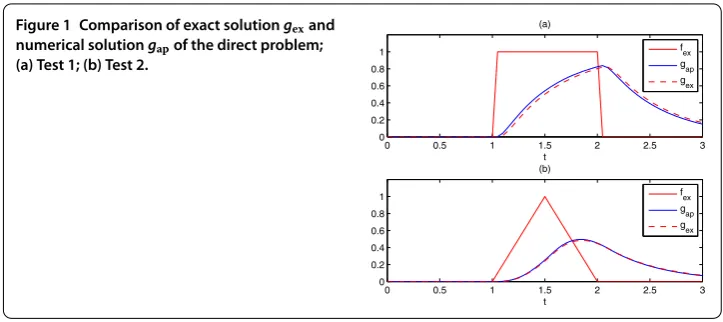
Figure 1 Comparison of exact solutiongexand
numerical solutiongapof the direct problem;
(a) Test 1; (b) Test 2.
2.3 Numerical examples
Puta= ,b= ,T= .
We consider the following examples.
Test Data:u(a,t) =f(t) =χ[,](χI denotes the characteristic function of an intervalI).
Test
f(t) = ⎧ ⎪ ⎪ ⎨ ⎪ ⎪ ⎩
(t– ), <t< .,
( –t), . <t< ,
otherwise.
In the following figures, we show the responseg(t) =u(b,t) to the sourcef(t).
In Figure , we callgexthe solution given by the truncated series () (with a rankN≥ ) and gap the approximate solution computed by FDM with parametersN= and M= ,.
3 Resolution of the inverse problem
3.1 Integral equation
As the functionu(b,t) =g(t) can be known, the resolution of the inverse problem ()-() can be reduced to the resolution of the Volterra integral equation of the first-kind
Af(t) := t
k(t–τ)f(τ)dτ=g(t) ()
with the kernel
k(t) =
∞
n= βn
W(b,sn)
W(a,sn)
esnt.
of the kernelk(t) vanish to zero according to Lemma (ii) (see also []). Therefore, some kind of regularization procedure will be necessary to solve the problem in the case of a perturbed datagδ.
For the numerical resolution of equation (), we approximate the kernelkby the trun-cated series
kN(t) = N
n= βn
W(b,sn)
W(a,sn)
esnt. ()
Remark The truncation error (the restRN =k–kN of the series) is estimated by
RN(t)≤C
n≥N
ne–Cnt
≤C
n≥N
ne–Cn
≤ CNe–CN
( –e–C) forNt≥ ()
withC= (λπ–)
. This means that, fortclose to , we need more terms in the series. For
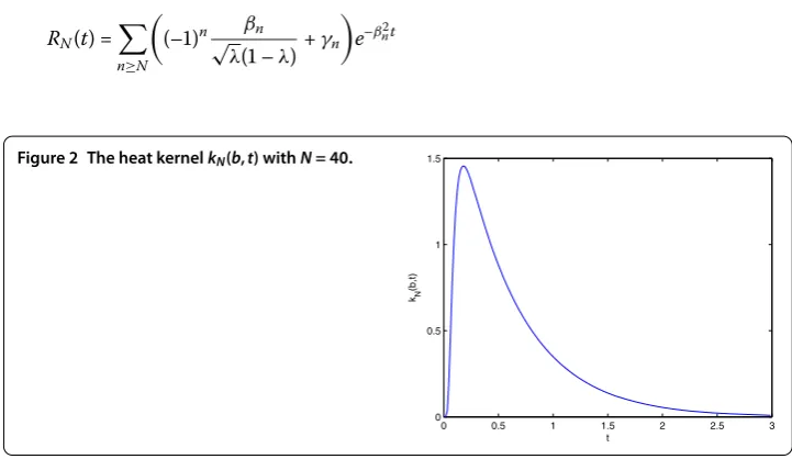
computation, we chooseN= forh<t≤.,N= for .≤t≤, andN= for t≥. For ≤t≤h, we can takek(t) = , since we know from () thatk(b,t) is close to zero ast→ (see Figure ). The parameterh= T
Mis the step time (we assume thath≥
N).
We denote byAN the operator with kernelkN.
Proposition ANconverge to A in the Banach spaceL(X),X=C[,T]equipped with the
norm · ∞.
Proof Using the asymptotic formula () withr=b, we can write
RN(t) =
n≥N
(–)n√ βn
λ( –λ)+γn
e–βnt
withγnbounded. Then
RN(t)≤CβNe–β
Nt+C
n≥N
e–βnt, C
=sup|γn|.
Using () with= , it follows that
T
RN(t)dt=
/N
RN(t)dt+
T
/N
RN(t)dt
≤C /N
βNe–β
Ntdt+ONe–CN=O(/β
N),
which leads to
∀t∈[,T], (A–AN)f(t)≤ f∞
T
RN(t)dt,
andA–ANL(X)=O(/N).
3.2 Tikhonov regularization
The approximate equationANf=gis solved by the Tikhonov regularization method.
Re-call the principle of the method.
Suppose thatA∈L(H) is a compact operator in Hilbert space, injective and with dense range. The equationAf =gis ill posed, that is,A–:R(A)→His not bounded (a small error in data g generates an important perturbation on the computed solutionf). The Tikhonov regularization method consists in solving the normal equation
AA+αIfα=Ag, ()
whereα> is a regularization parameter, andIis the identity operator. Equivalently,fα
is the unique minimum of the Tikhonov functional
Jα[f] =Af –gH+αfH.
The solutionfαcan be written as follows:
fα=AA+αI–Ag,
which can be expressed in terms of the singular system (μj,uj,vj)j∈N∗as
fα:=R αg=
j
μj
μ
j +α
(g,vj)uj.
Now let g∈R(A), and let gδ ∈H be a measured data withg–gδ
H≤δ. We define
fα,δ=R
αgδ. A posteriori discrepancy principle gives a selection ofα (a solution of the
equationAfα,δ–gδ
H=δ). Standard Tikhonov regularization theory (see [, Theorem
.]) shows the convergencefα,δ→f inHasδ→ with the strategyα=α(δ). For other
3.3 Numerical experiment
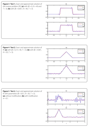
We consider the following examples.
Test As a first example, we consider the couple{f,g}, where
u(a,t) =f(t) =χ[,],
andg(t) =u(b,t) is computed by finite difference scheme (see Section .).
Test We consider the example given by
f(t) = ⎧ ⎪ ⎪ ⎨ ⎪ ⎪ ⎩
(t– ), <t< .,
( –t), . <t< ,
otherwise.
To check the efficiency of the proposed algorithm, we choose in numerical experiments the parametersa= ,b= ,T= orT= as required, and the rank of truncation ≤ N≤.
For an exact data functiong(t) =u(b,t), we use a finite difference scheme withN= points in the interval [, ] andM= , points in [,T]. The discrete noisy version isgδ=g+δrandn(size(g)), the command ‘randn(·)’ generates arrays of random numbers
whose elements are normally distributed with mean , varianceσ= , and standard de-viationσ= . For the singular decomposition and Tikhonov-Morozov algorithms, we used the Matlab package developed by Hansen [].
3.4 Results and discussion
Figures and show the numerical results that confirm the stability of the method with respect to the noise levelδ≤.. However, the rank inkN must be large enough (here
N≥) to ensure the convergence of the Tikhonov algorithm. Figure (a) shows that, forδ= ., the oscillations increase, which requires a new regularization. Indeed, if we use the mollification method [], then the oscillations are damped (see Figure (b)). The operation consists in taking the convolutiongν=ρν∗gwithρν(t) =ν√πexp(–t
ν), where
ν→ is the radius of mollification. Ifgvanishes near the ends of the interval [,T], thengν
is a smooth function and is a good approximation ofg; this fact is realized if the observation timeTis large enough (in practice, we takeT= Tif suppf ⊂[,T]). In the presence of the noise, according to the analysis in [], we chooseν=c√δwithc= estimated by test.
4 Conclusion
Figure 3 Test 1.Exact and approximate solution of the inverse problem (IP);(a)with (δ= 0,N= 40 and
T= 3);(b)with (δ= 0.001,N= 40,T= 3).
Figure 4 Test 2.Exact and approximate solution of IP;(a)with (δ= 0,N= 40,T= 3);(b)with (δ= 0.001,
N= 50,T= 3).
Figure 5 Test 2.Exact and approximate solution of IP with parameters (δ= 0.01,N= 30,T= 5);
(a)without mollification;(b)with mollification ν= 0.1.
Appendix 1: Asymptotic expansions For fixedνand|z| → ∞, we have []
Jν(z)∼
πzcos
z–π
– νπ
, Yν(z)∼
πzsin
z–π
– νπ
, ()
Iν(z)∼
ez
√
πz, Kν(z)∼
π ze
We consider the rapportG(r,s) = WW((ra,,ss)) withW(r,s) =I(b√s)K(r√s) +K(b√s)I(r√s). Due to (), we have, forr∈]a,b] and|s| →+∞,
G(r,s)=
a rexp
–(r–a)ρ/cosθ
+O ρ ,
whereρ=|s|andθ=arg(s)∈[–π
, π
]. Then there exist positive constantsCandμsuch that, for|s|large enough, say|s| ≥ρ,
G(r,s)est≤Cexp
–(r–a)ρ/cosθ
+tρcosθ
≤Cexp
–m√ρcosθ
+|cosθ| m=min(r–a,t)
≤Cexp(–μ√ρ)
uniformly forθ∈ π , π . ()
Appendix 2: Zeros of cross-product
We want to seek the rootssnof the following function (cross-product):
W(s) =I(b √
s)K(a √
s) +K(b √
s)I(a √
s).
We show thatsn= –βnwithβn→+∞asn→+∞. For this, we consider the self-adjoint
operator defined inH=L((a,b);r dr) by
AU= – r d dr rdU dr
, D(A) =U∈H]a,b[;U() =U() = .
IfAU=λU, then (AU,U) =U=λU. SinceA–is compact,Ahas a sequence of pos-itive eigenvaluesλn→+∞. On the other handλn= –sncoincides with the roots ofW(s).
Indeed, this can be seen by solving the Sturm-Liouville problem (system () in Section ) withλ= –sandF= .
Now we give the behavior ofsn. Using the relations between the Bessel functions
In(z) =i–nJn(iz) and Kn(z) =
π i
n+ J
n(iz) +iYn(iz)
forn∈N,
we obtain, fors= –β,
W–β=iπ
J(aβ)Y(bβ) –J(bβ)Y(aβ)
. ()
Using the asymptotic expansions () for largeβ, we get
W–β∼√i abβcos
b a–
β
,
and hence the zeros ofW(s) are a sequencesn= –βn,n= , , . . . , such that
βn∼
n–
aπ
Acknowledgements
The work is supported by the National Research Foundation (CNEPRU) of Algeria (No. B01120120016).
Competing interests
The authors declare that they have no competing interests.
Authors’ contributions
All authors contributed equally to the writing of this paper. All authors read and approved the final manuscript.
Publisher’s Note
Springer Nature remains neutral with regard to jurisdictional claims in published maps and institutional affiliations.
Received: 12 July 2017 Accepted: 21 October 2017 References
1. Eldén, L, Berntsson, F, Regi ´nska, T: Wavelet and Fourier methods for solving the sideways heat equation. SIAM J. Sci. Comput.21(6), 2187-2205 (2000)
2. Berntsson, F: A spectral method for solving the sideways heat equation. Inverse Probl.15, 891-906 (1999) 3. Fu, C-L: Simplified Tikhonov and Fourier regularization methods on a general sideways parabolic equation.
J. Comput. Appl. Math.167(2), 449-463 (2004)
4. Murio, DA: The Mollification Method and the Numerical Solution of Ill-Posed Problems. Wiley, New York (1993) 5. Yaparova, N: Numerical methods for solving a boundary-value inverse heat conduction problem. Inverse Probl. Sci.
Eng.22(5), 832-847 (2014)
6. Cheng, W, Fu, C-L: Solving the axisymmetric inverse heat conduction problem by a wavelet dual least-squares method. Boundary Value Problems2009, Article ID 260941 (2009). doi:10.1155/2009/260941
7. Cheng, W, Fu, C-L: Two regularization methods for an axisymmetric inverse heat conduction problem. J. Inverse Ill-Posed Probl.17(2), 159-172 (2009)
8. Cheng, W: Regularization and stability estimates for an inverse source problem of the radially symmetric parabolic equation. J. Inequal. Appl.2015, 136 (2015)
9. Cheng, W, Zhao, L-L, Fu, C-L: Source term identification for an axisymmetric inverse heat conduction problem. Comput. Math. Appl.59, 142-148 (2010)
10. Xiong, X-T: On a radially symmetric inverse heat conduction problem. Appl. Math. Model.34, 520-529 (2010) 11. Cheng, W, Fu, C-L: A modified Tikhonov regularization method for an axisymmetric backward heat equation. Acta
Math. Sin. Engl. Ser.26(11), 2157-2164 (2010)
12. Johansson, BT, Lesnic, D, Reeve, T: A method of fundamental solutions for the radially symmetric inverse heat conduction problem. Int. Commun. Heat Mass Transf.39, 887-895 (2012)
13. Tuan, NH, Kirane, M, Luu, VCH, Bin-Mohsin, B: A regularization method for time-fractional linear inverse diffusion problems. Electron. J. Differ. Equ.2016, 290 (2016)
14. Ditkine, V, Proudnikov, A: Transformation Intégrales et Calcul Opérationnel. Traduit du Russe. Éditions MIR, Moscou (1978)
15. Abramowitz, M, Stegun, IA: Handbook of Mathematical Functions. Dover, New York (1972)
16. Herbin, R: Analyse numérique des équations aux dérivées partielles. Engineering school, Marseille 2011. https://cel.archives-ouvertes.fr/cel-00637008
17. Lamm, PK: A survey of regularization methods for first-kind Volterra equations. In: Colton, D, Engl, HW, Louis, AK, McLaughlin, JR, Rundell, W (eds.) Surveys on Solution Methods for Inverse Problems, pp. 53-82. Springer, Vienna (2000). doi:10.1007/978-3-7091-6296-5_4
18. Kirsh, A: An Introduction to the Mathematical Theory of Inverse Problems. Applied Mathematical Sciences Book Series, vol. 120. Springer, Berlin (2011)
19. Lamm, PK, Eldén, L: Numerical solution of first-kind Volterra equations by sequential Tikhonov regularization. SIAM J. Numer. Anal.34(4), 1432-1450 (1997)