Fast mode decision based on human noticeable luminance difference and rate distortion cost for H 264/AVC

R E S E A R C H

Open Access

Fast mode decision based on human noticeable

luminance difference and rate distortion cost

for H.264/AVC

Mian-Shiuan Li

, Mei-Juan Chen

, Kuang-Han Tai

and Kuen-Liang Sue

Abstract

This article proposes a fast mode decision algorithm based on the correlation of the just-noticeable-difference (JND) and the rate distortion cost (RD cost) to reduce the computational complexity of H.264/AVC. First, the relationship between the average RD cost and the number of JND pixels is established by Gaussian distributions. Thus, the RD cost of the Inter 16 × 16 mode is compared with the predicted thresholds from these models for fast mode selection. In addition, we use the image content, the residual data, and JND visual model for horizontal/vertical detection, and then utilize the result to predict the partition in a macroblock. From the experimental results, a greater time saving can be achieved while the proposed algorithm also maintains performance and quality effectively.

Keywords:Mode decision, H.264/AVC, Rate distortion cost, Human vision system

1. Introduction

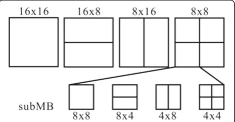
With sophisticated technology increasing, multimedia communication has become an important part of human life. In addition to general telecommunications, wide-spread Internet reliance has made video communication essential. However, the quality of video communication is highly dependent on the efficiency and quality of video transmission. Therefore, many international stan-dards have been developed in recent years. H.264/AVC is one of the popular video coding standards [1]. It is widely applied in video transmission and compression products, e.g., mobile phones, video surveillance, digital TV, etc. Although H.264/AVC has a high coding effi-ciency, enormous computational complexity is required. In particular, the mode decision procedure occupies the majority of computational complexity due to the evalu-ation of several inter modes and nine intra predictive directions for Intra 4 × 4 as shown in Figures 1 and 2, respectively. Many studies related to the reduction of computational complexity of mode decision have been proposed.

Bharanitharan et al. [2] proposed a classified region al-gorithm to reduce the inter mode candidates. The ana-lyses of spatial/temporal homogeneity and edge direction were used to choose the inter modes needed for the rate distortion optimization (RDO) calculation. Choi et al. [3] considered those macroblocks (MBs) with the same mo-tion vectors in the same object. Therefore, they utilized the characteristics of each 4 × 4 block after utilizing a Haar wavelet transform to test the homogeneity in an MB in order to select the candidate modes. Pan et al. [4] reordered the modes according to their probabilities and utilized the mean value and the standard deviation of rate distortion costs (RD costs) to be the early termination cri-terion of RDO. Lee and Lin [5] utilized the probabilities of several modes to calculate the average computation time in each mode. Yeh et al. [6] predicted the best mode based on Bayesian theory, and refined the prediction with the Markov process. The computational complexity was effi-ciently reduced. The SKIP mode condition was presented to make a consideration of the neighborhood and co-located information to achieve the reduction in the coding time in [7]. The relation between depth value and mode distribution was analyzed, and the mode candidates were chosen according to different levels of depth in an MB in [8]. Statistics were gathered for both of the RD cost and

* Correspondence:[email protected]

1

Department of Electrical Engineering, National Dong Hwa University, Shoufeng, Hualien, Taiwan

Full list of author information is available at the end of the article

occurrence probability of each mode in [9]. The normal distribution of RD cost was adopted to calculate the thresholds for early termination. A 2D map was generated according to the neighboring motion vectors in [10]. Inter modes were reordered or removed via this 2D map. Ri et al. [11] defined a spatial-temporal mode prediction. The calculated RD cost and the co-located mode were utilized to produce the threshold for mode selection. Visual char-acteristics of tunnel surveillance videos were considered to analyze the structure of neighborhood inter/intra blocks for adapting the characteristics of static and fixed backgrounds in the observation systems in [12]. Codes in compliance with a coding order of previously neighbor-ing blocks were assigned to increase the opportunity for an early termination in [13]. The relations between the discrete cosine transform (DCT), the sum of absolute difference, and the sum of square difference were established as the conditions for an early termination in [14]. Not only DCT but also the magnitude order of RD cost was discussed in [15]. The connection between the quantization parameter (QP) and the RD cost was

experimented with to act as the threshold in [16]. The ac-tivity was calculated by utilizing the motion vectors of the neighboring and co-located blocks of the current block.

In addition to the methods of exploration of rate dis-tortion and motion information, the human visual sys-tem (HVS) is also useful for improving video coding. Just-noticeable-difference (JND) is one of the important characteristics in HVS. A model of the luminance differ-ence perception of human vision was developed in [17]. Knowledge about human visual luminance distortion was provided by this model. The human visual charac-teristics of JND were employed to analyze the content of video for the purpose of improving computational com-plexity in [18]. In [19], JND was utilized to re-measure image distortion. A perceptual rate distortion model was used to judge mode candidates. The necessary informa-tion was provided by gradient, variance, average con-trast, and edge data in an MB for considering HVS [20].

This article proposes a fast mode decision algorithm which utilizes the correlation of JND pixels and RD cost to reduce the number of mode candidates. The rest of this article is organized as follows. In Section 2, the JND visual model and total number of non-JND pixels are discussed. The proposed fast mode decision algorithm is described in Section 3. The extensive experimental re-sults are presented in Section 4. In Section 5, conclusion remarks are provided.

2. JND visual model

2.1. Human visual luminance difference

A JND model was applied as a human visual model as previously mentioned in [17]. JND refers to the visual threshold based on the background luminance. The dif-ference between the foreground and background is Figure 1Several inter modes in mode decision for H.264/AVC.

smaller than that within a certain region, so the human eye is not able to detect it. That is, human eyes are allowed to tolerate certain luminance distortion. This type of feature can be incorporated into a fast mode de-cision if the observation of the human eye on a block can be characterized by such a feature. The redundancy of computational complexity will then be decreased. The JND visual model indicates the visual distortion of lumi-nance and is shown in Figure 3.

JNDðY ið Þ;jÞ ¼T0 1ðY ið Þ;j=127Þ constants (T0= 17,γ= 3/128). The horizontal axis repre-sents the gray level of the background. Each value corre-sponds to a JND value on the vertical axis. If the gray

level difference between the background and the object is smaller than that of the human visual distortion de-noted as the JND value, the object could not be detected visually. This concept of the human visual distortion of the gray level difference can be extended to the temporal domain. We can utilize this characteristic of the notice-able difference to observe the variation of the gray level on the temporal domain. In a video stream, there simi-larly is the variation of the gray level on every pixel loca-tion. Through these variations of the gray level frame-by -frame, consequentially, part of the content is easy to be detected for the variation, but some part seems to be without any alteration. The JND model can thus detect this magnitude of variation of luminance for the human eye. Therefore, that is the purpose for applying notice-able difference to the temporal domain while this usage of pixel domain can also be expended to an MB. There-fore, the human visual distortion criterion of an MB is determined by this characteristic.

In the proposed algorithm, the residual value of every pixel in an MB is compared. That is, the intensity values of the original pixels in the current MB are treated as the background luminance in the JND model, so that the JND value (visual threshold) can be obtained by using the model. If the residual value is less than the JND value, the variation of pixels cannot be perceived by human eyes.

2.2. Human visual characteristics in an MB

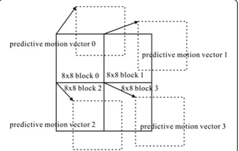
After describing the JND visual model, the details of how to utilize this visual characteristic in an MB will be discussed. First, an MB is divided into four 8 × 8 blocks. Pixels are subtracted into an 8 × 8 block from the block of the reference frame at the predicted location which is produced by the predictive motion vector as illustrated in Figure 4. The median motion vectors of the nearest Figure 3Visibility thresholds due to background luminance

[17].

Figure 4Subtraction from an 8 × 8 block of the reference frame at the predicted location.

neighboring coded MBs are taken as the predicted mo-tion vectors. It is a little different from the momo-tion vector predictor (MVP) in H.264/AVC, and an example is exhibited in Figure 5. In this step, the motion estimation of each 8 × 8 block does not need to be executed. The current MB is separated into four 8 × 8 blocks (C0, C1, C2, C3) while the coded neighboring MBs, respectively, are left (L), top (T), and upper right (UR). The left MB is the 8 × 8 mode labeled as L0, L1, L2, and L3. The top MB is the 8 × 16 mode labeled as T0and T1. The upper

right MB is the 16 × 8 mode labeled as UR0and UR1. In this example, the predictive motion vector of block C0is calculated with the motion vectors of L1, T0, and UR1 while that of block C1is obtained with the motion vec-tors of L1, T1, and UR1. The predictive motion vector of block C2is gotten with the motion vectors of L3, T0, and UR1while that of block C3is calculated with the motion vectors of L3, T1, and UR1.

An 8 × 8 block is chosen to be JND measurement in-stead of a 16 × 16 or 4 × 4 block due to the consideration

(a)

8x16 mode

(b)

subMB

of the structure of several modes in H.264/AVC. This mode structure can be imagined as a pyramid. Both the general and detail block partitions are considered. Hence, there are trade-offs when selecting the block in the mode structure. It should not be as unduly rough as a 16 × 16 block. Also it is not as excessively detailed as a 4 × 4 block. This concept of the different layers of block size is confined to the original mode structure of H.264/ AVC. The mode structure of H.264/AVC is only sup-ported by blocks of sizes 16, 8 and 4. No matter what the image resolution is, the biggest block size can only be 16 × 16 while the smallest can only be 4 × 4. There-fore, 8 × 8 is the nearest block size to the two sizes. If 16 × 16 is selected for JND measurement, this MB can-not estimate the different motions of smaller sizes, while if the size of 4 × 4 is adopted, the predictive motion

vectors could be too diverse. If, on the other hand, 8 × 8 is selected, it can compensate the drawbacks for blocks that are too large or too small. Therefore, an 8 × 8 block is an applicable one as a basic block for measuring the visual distortion.

After the residual values of the four 8 × 8 blocks in an MB are obtained, the intensity values of the original pixels in these four 8 × 8 blocks are treated as the back-ground luminance in the JND model which allows a JND value to be found for every pixel location. If the displaced residual value is smaller than the JND value, the change of the gray level cannot be detected by hu-man eyes because the difference between the current pixel and the one at the predicted location is smaller than the human noticeable luminance distortion. Pixels are counted in this manner for every 8 × 8 block. The number of non-JND pixels (NNJND) in each 8 × 8 block is provided. The summation of four 8 × 8 blocks is the total number of non-JND pixels (TNNJND) in an MB. A criterion of the visual perception is provided by NNJND Figure 7The flowchart of the proposed mode

decision algorithm.

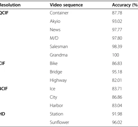
Table 1 The accuracy of SKIP and 16 × 16 modes when

TNNJNDis 256 (QP24, 300 frames)

Resolution Video sequence Accuracy (%)

QCIF Container 87.78

Table 2 The accuracy of intra 4 × 4 mode when TNNJNDis

0 (QP24, 100 frames)

Resolution Video sequence Accuracy (%)

or TNNJND which comes from the original JND visual model. If an MB has more TNNJND, it will possess more characteristics of non-noticeable visual luminance dis-tortion because the number of the points means the number of unnoticeable difference pixels. If there are lots of TNNJND in an MB, it belongs to a relatively low complexity of movement or image content since most of the temporal difference of the predicted location cannot be detected by human eyes. On the contrary, if there are few TNNJND in this MB, the temporal difference can be detected easily and thus this MB has a relatively high complexity of movement or image content.

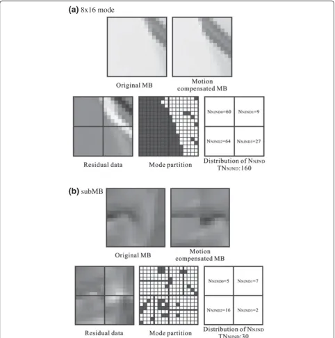
The examples of NNJND and TNNJND under different conditions of image content and mode partition are exhibited in Figure 6. According to the process described above, the elements of visual judgment are obtained in an MB. NNJND0, NNJND1, NNJND2, and NNJND3 are the numbers of NNJND pixels in the four 8 × 8 blocks. TNNJND is the total number ofNNJNDpixels by summa-tion. In this instance, Figure 6a depicts an example of low variability. It can be observed that the difference is not obvious according to the current MB, the motion compensated MB, and the residual data. Therefore, it processes lots of NNJND in each 8 × 8 block. The final mode partition is 8 × 16 which is a relatively large block type. Figure 6b gives an example of high variability. In this case, the content is obviously variable. It is part of the image in the Foreman sequence. Correspondingly, few NNJND are possessed in each 8 × 8 block due to its high temporal variability. Therefore, it is conceivable that its block type should be selected as a relatively de-tailed mode partition.

According to the above description, the relationship is obtained between the temporal difference, residual value, and NNJND in each 8 × 8 block. If the temporal discontinuity is larger, the block type has more oppor-tunity for a comparatively detailed mode partition. Few

NNJND and TNNJND are obtained due to the massive temporal variability while exceeding the visual unnotice-able distortion.

3. Proposed fast mode decision algorithm

The flowchart of the proposed algorithm is exhibited in Figure 7. The SKIP and 16 × 16 modes will be conducted first as the original flow of the coding stand-ard. We can observe that if TNNJND is equal to 256 in an MB, it almost tends to be selected as SKIP or 16 × 16 mode because it means the difference of this MB in the temporal domain is negligible. Therefore, we just choose SKIP and 16 × 16 modes in mode candidates, and end up with the mode decision. We also provide some statis-tical examples of its accuracy in Table 1. In Table 1, the high accuracy can prove whether this process of early termination is practical. For usual cases, we try the intra 16 × 16 mode. When TNNJND is equal to zero, we add intra 4 × 4 mode into our mode candidates, because it means the temporal difference of this MB could be very large. The high accuracy is exhibited in Table 2 which indicates the probability of intra 4 × 4 when TNNJNDis equal to zero. Since it does not have any of the charac-teristics of unnoticeable visual distortion, it cannot get a great coding efficiency from the motion compensation and spatial prediction of a large block (intra 16 × 16). In this case, we take the intra 4 × 4 mode into consider-ation of the intra prediction.

If the required inter mode candidates in H.264/AVC can be predicted accurately, the computational com-plexity can be reduced. We observe that the average RD cost of the 16 × 16 mode (RDcost16×16, the 16 × 16 mode must have been calculated for every MB in the original coding standard) since each final mode of the MB’s mode decision in inter frames is based on TNNJND which exhibits a trend that when the best mode belongs to a relatively bigger block size, for instance, SKIP or 16 × 16 mode, its RDcost16×16 is generally lower than the one that its best mode belongs to in detail partitions. We demonstrate this phenomenon in Figure 8 with six QCIF (Foreman, Grandma, Mother & Daughter (M/D), News, Salesman, Football), three CIF (Bike, Bridge, Highway), three 4CIF (Ice, Soccer, City), and two HD (Stockholm, Parkrun) sequences. Therefore, the distri-bution model is built between the average RDcost16×16 and TNNJND, and then the requisite mode candidates will be determined accurately. According to the relation between the average RDcost16×16and TNNJND, the mode candidates are decided to be the relatively large or de-tailed mode partition.

The statistics of the average RDcost16×16are gathered when the best mode is 16 × 16 based on each TNNJND using six QCIF sequences as Th1(TNNJND). The Figure 8Average RDcost16×16versus TNNJNDin each mode with

tendency judgement of the mode partition by the sum-mation of Gaussian functions is defined as

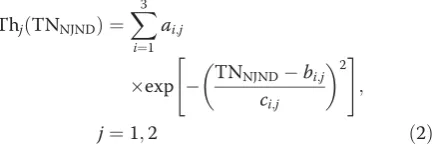
ThjðTNNJNDÞ ¼

X3

i¼1

ai;j

exp TNNJNDbi;j

ci;j

2

" #

;

j¼1;2 ð2Þ

where j is the number of threshold. ai,j, bi,j, ci,j are

Table 3 Coefficients of Th1(TNNJND)

QP a1,1 b1,1 c1,1 a1,2 b1,2 c1,2 a1,3 b1,3 c1,3

24 18840 11.63 18.42 14820 36.13 42.74 30100 116.8 151.6

28 19660 11.76 18.55 14240 35.28 35.92 42330 99.03 155.2

32 38030 9.64 22.00 25850 42.81 39.09 55380 117.8 129.2

36 44520 7.79 20.16 37910 37.68 37.29 75650 111.6 122.6

40 27840 9.14 10.97 99410 93.96 128.8 51020 22.74 37.24

Table 4 Coefficients of Th2(TNNJND)

QP a2,1 b2,1 c2,1 a2,2 b2,2 c2,2 a2,3 b2,3 c2,3

24 19850 21.83 15.00 14100 9.048 5.038 55520 −121.9 395.9

28 32580 10.19 19.58 25410 31.86 41.4 51880 115.5 137.4

32 45160 9.261 21.54 64410 39.68 56.82 67120 145.5 89.07

36 58980 5.391 26.55 84090 39.69 53.22 87280 135.3 83.3

40 112300 6.871 34.95 111600 58.91 55.32 100000 144.8 63.99

Table 5 Distribution of various modes

Mode X Foreman (%) Grandma (%) M/D (%) News (%) Salesman (%) Football (%) Average (%)

SKIP 13.83 49.26 38.41 49.38 47.60 7.79 34.38

16 × 16 28.55 27.93 27.00 26.47 29.24 17.34 26.09

16 × 8 and 8 × 16 30.17 10.79 16.75 9.58 7.36 16.32 15.16

8 × 8 6.13 2.80 4.06 1.93 2.18 4.26 3.56

subMB 18.92 9.02 13.54 12.54 13.59 31.55 16.53

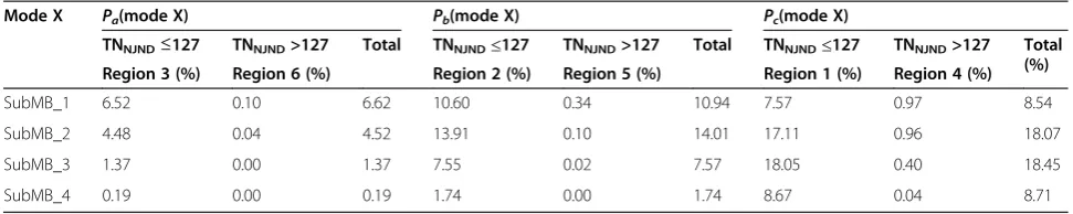
Table 6 The probability distribution of the proposed Th_j(TNNJND) for various modes

mode X Pa(mode X) Pb(mode X) Pc(mode X)

TNNJND≤127 TNNJND>127 Total

(%)

TNNJND≤127 TNNJND>127 Total

(%)

TNNJND≤127 TNNJND>127 Total

(%) Region 3 (%) Region 6 (%) Region 2 (%) Region 5 (%) Region 1 (%) Region 4 (%)

SKIP 48.86 19.36 68.22 16.32 7.90 24.22 2.46 5.10 7.56

16×16 45.64 12.19 57.83 20.60 7.22 27.82 8.52 5.84 14.36

16×8 and 8×16 35.04 3.47 38.51 30.42 3.72 34.14 21.50 5.85 27.35

8×8 26.21 0.49 26.70 38.02 0.97 38.99 30.27 4.05 34.32

curve fitting. Because the TNNJND samples which are close to 256 are much fewer, the curve trend would fall according to its smaller number of samples. In our experiments, the higher threshold is selected at this condition.

In Table 5, the distributions of various modes are compared. It can be observed that most modes belong to relatively large mode partitions. The total distribution is 60.47% for the SKIP and 16 × 16 modes. A distribution of 15.16% for both the 16 × 8 and 8 × 16 modes is obtained. The 8 × 8 mode and subMB occupy a total dis-tribution of 20.09% in the various mode disdis-tributions.

Statistics of the same six QCIF sequences with 300 frames by QP 24 which analyze the accuracy of the pro-posed Thj(TNNJND) are listed in Table 6. Mode X is the best mode for an MB after conducting the RDO. Pa

(mode X),Pb(mode X), andPc(mode X) are the

probabil-ities of mode X given all MBs with mode X in inter frames under different conditions. Pa(mode X) denotes

that its current RDcost16×16 is equal to or lower than Th1(TNNJND). Pb(mode X) means that its current RDcost16×16 is larger than Th1(TNNJND) and is equal to or lower than Th2(TNNJND). Pc(mode X) indicates that its current RDcost16×16is larger than Th2(TNNJND). The probability distribution can be displayed by Th1and Th2

as listed in Table 6. The regions indicated in Table 6 are shown in Figure 10. The total probability distribution is 92.44% for SKIP mode and 85.65% for 16 × 16 mode in the entire inter frames. If the current RDcost16×16 is equal to or lower than Thj(TNNJND), some smaller modes are still required to be tested. In addition, most of the other smaller modes are distributed with TNNJND under 127. For Pa(mode X), Pb(mode X), Pc(mode X),

and the conditions of TNNJND of 127 exhibited in Table 6, there are other modes (16 × 8, 8 × 16, 8 × 8, and subMB) to be included according to Thj(TNNJND) as well as most of their probabilities dispensed with TNNJND under 127.

In the proposed scheme, both 8 × 8 mode and subMB are not calculated when the condition that the current RDcost16×16is equal to or lower than Th1(TNNJND) with TNNJND under 127 as shown by region 3 in Figure 10. The reason is that the occurrence probabilities of 8 × 8 mode and subMB are relatively low as demonstrated in Table 5 and the distribution of the proposed Thj

(TNNJND) for various modes as demonstrated in Table 6. In Table 5, the total probabilities occupy only 20.09% among various modes. Most of the 8 × 8 mode and subMB are not distributed with high probabilities in re-gion 3 according to the condition of Thj(TNNJND) in Table 6. Therefore, the occurrence probabilities of 8 × 8 mode and subMB determined in region 3 are small enough to be neglected.

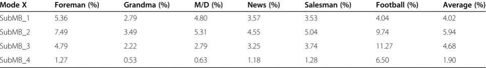
The statistics that subMB are classified into four subMB_nwheren is equal to 1, 2, 3, or 4 are shown in Tables 7 and 8. Thenindicates the number of subMB in an MB. The importance of subMB is analyzed according to the utilization rate. For instance, if there is only one subMB either 8 × 4, 4 × 8, or 4 × 4 mode in an MB and the other three subMBs are 8 × 8 blocks, it belongs to the classification of subMB_1, and so on. Because the utilization probability with four subMBs in an MB is ob-viously low, the performance degradation will not be in-creased much when the termination is made early to ignore the computation of subMBs.

After the analyses of Tables 5, 6, 7, and 8, the relation between TNNJND, current RDcost16×16, and Thj(TNNJND) is exhibited in Figure 10. In Figure 10, the regions 1, 2, and 4 are allocated by checking all inter modes. SKIP, 16 × 16, 16 × 8, and 8 × 16 modes are included in region Figure 10Mode distribution by proposed algorithm according

to TNNJNDand Thj(TNNJND).

Table 7 Distribution of subMBs

Mode X Foreman (%) Grandma (%) M/D (%) News (%) Salesman (%) Football (%) Average (%)

SubMB_1 5.36 2.79 4.80 3.57 3.53 4.04 4.02

SubMB_2 7.49 3.49 5.31 4.55 5.04 9.74 5.94

SubMB_3 4.79 2.22 2.79 3.25 3.74 11.27 4.68

3. With regard to regions 5 and 6, procedures can be terminated early after conducting the RDOs of SKIP and 16 × 16 modes. The condition of TNNJND is firstly deter-mined in the proposed algorithm because TNNJNDis the key factor to decide whether or not to check other modes except SKIP and 16 × 16 modes. The decision is made according to the above analyses of the mode distri-butions from Table 6. Afterwards, if TNNJNDis equal to or lower than 127, the comparatively strict Th1(TNNJND) is chosen to be the threshold. If the current RDcost16×16 is equal to or lower than Th1(TNNJND) (region 3 in Figure 10), 16 × 8 and 8 × 16 modes are added in the final mode candidates. If current RDcost16×16 is larger than Th1(TNNJND) (regions 1 and 2 in Figure 10), all in-ter modes are mode candidates. Also, if TNNJNDis larger than 127, the relatively loose Th2(TNNJND) is selected to be the threshold. If the RDcost16×16of the current MB is equal to or lower than Th2(TNNJND) (regions 5 and 6 in Figure 10), the procedure will be terminated early and no other mode candidate is added. Otherwise, as shown in region 4 in Figure 10, 16 × 8, 8 × 16, 8 × 8 modes, and subMBs are entered as final mode candidates.

According to Figure 10, the relation between TNNJND and Thj(TNNJND) can be discussed. If TNNJNDis large in an MB, more visual non-JND will exist. If very low current RDcost16×16 is possessed by an MB, it tends to choose relatively large blocks according to the illustra-tion in Figure 8. There are more opportunities to choose large blocks after the procedure of the mode decision. This characteristic is also possessed by the proposed al-gorithm. If there are more TNNJNDin an MB, or the MB

possesses very low current RDcost16×16, the procedure has more opportunities to choose a relatively larger block and to terminate the process earlier. Therefore, the cost of unnecessary computational complexity to choose the best mode among mode candidates can be re-duced according to the total number of non-JND pixels and current RDcost16×16and by the fitting curves to give appropriate Thj(TNNJND) produced from statistics.

3.1. Characteristics of image direction

Following our flowchart shown in Figure 7, the direction of image texture should be considered after the previous steps. The directional characteristic in an MB will be discussed. When the directional characteristic in an MB is strong enough, only one of the two directional modes, 16 × 8 and 8 × 16 modes, is needed because these two modes cannot coexist. Therefore, if only one of the two directional modes in the final mode candidates is chosen, the computational cost can be further reduced. Table 8 The probability distribution of the proposed Th_j(TNNJND) for subMBs

Mode X Pa(mode X) Pb(mode X) Pc(mode X)

TNNJND≤127 TNNJND>127 Total TNNJND≤127 TNNJND>127 Total TNNJND≤127 TNNJND>127 Total

(%) Region 3 (%) Region 6 (%) Region 2 (%) Region 5 (%) Region 1 (%) Region 4 (%)

SubMB_1 6.52 0.10 6.62 10.60 0.34 10.94 7.57 0.97 8.54

SubMB_2 4.48 0.04 4.52 13.91 0.10 14.01 17.11 0.96 18.07

SubMB_3 1.37 0.00 1.37 7.55 0.02 7.57 18.05 0.40 18.45

SubMB_4 0.19 0.00 0.19 1.74 0.00 1.74 8.67 0.04 8.71

Figure 11The examples of edge characteristics in an MB.

The edge information of an MB is calculated by Sobel edge detector to decide whether both 16 × 8 and 8 × 16 modes are included as mode candidates or not. If the edge magnitude of any pixel in an MB is larger than 180, the horizontal or vertical decision is made according to Equations (3), (4), (5). Part of the chin image in Foreman sequence is shown in Figure 11a, which is the real mode structure after encoding. The white pixels in Figure 11b indicate those pixels whose Sobel edge magnitudes are larger than 180.

Three groups of edge directions are calculated in the proposed algorithm including the horizontal and verti-cal verti-calculations of the original gray value (H1/V1), the residual compensated by the MVP in an MB (H2/V2), and theNNJNDdistribution for each 8 × 8 block (H3/V3). Figure 12a shows an example of NNJND distribution at the brim of the hat in the Foreman sequence. The num-bers of NNJND in Figure 12b,c are distributed in the horizontal structure. The best mode is 16 × 8. H3 is much larger than V3.

Table 9 Performance and coding efficiency comparisons of proposed algorithm with JM16.2 for IPPP frame structures (QP: 24, 28 and 32)

IPPP QP24 QP28 QP32

Video ΔPSNR ΔBR (%) TS (%) ΔPSNR ΔBR (%) TS (%) ΔPSNR ΔBR (%) TS (%)

Foreman −0.048 0.408 68.386 −0.042 0.702 68.226 −0.038 0.964 68.555

Grandma −0.044 −0.365 73.561 −0.025 0.099 70.208 −0.031 −0.107 68.989

M/D −0.060 0.166 77.486 −0.023 0.213 76.261 −0.025 0.163 76.071

News −0.079 0.065 78.944 −0.055 0.131 76.536 −0.048 0.097 74.042

Salesman −0.044 0.106 76.105 −0.015 0.115 72.351 −0.019 −0.077 69.184

Coastguard −0.003 0.172 59.624 −0.009 0.136 58.840 −0.020 0.085 59.343

Mobile −0.007 0.103 63.934 −0.002 0.206 62.538 −0.009 0.307 60.776

Silent −0.038 0.866 74.891 −0.033 1.011 71.784 −0.027 1.299 70.962

Stefan −0.038 0.618 63.667 −0.033 0.731 63.564 −0.040 0.838 63.081

Table −0.022 0.263 68.944 −0.041 0.554 67.111 −0.035 0.886 67.699

Stockholm 0.001 0.437 56.966 −0.006 0.438 56.875 −0.025 0.017 61.408

Parkrun −0.003 0.095 57.537 −0.004 0.123 55.530 −0.003 0.204 54.194

Average −0.032 0.245 68.337 −0.024 0.372 66.652 −0.027 0.390 66.192

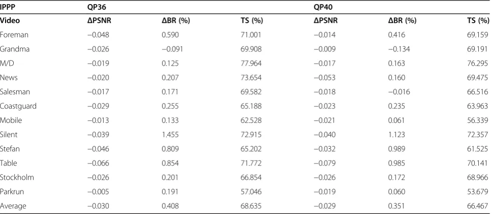
Table 10 Performance and coding efficiency comparisons of proposed algorithm with JM16.2 for IPPP frame structures (QP: 36 and 40)

IPPP QP36 QP40

Video ΔPSNR ΔBR (%) TS (%) ΔPSNR ΔBR (%) TS (%)

Foreman −0.048 0.590 71.001 −0.014 0.416 69.159

Grandma −0.026 −0.091 69.908 −0.009 −0.134 69.191

M/D −0.019 0.125 77.964 −0.017 0.163 76.295

News −0.020 0.207 73.654 −0.053 0.160 69.475

Salesman −0.017 0.171 69.582 −0.018 −0.016 66.516

Coastguard −0.029 0.255 65.188 −0.023 0.235 63.963

Mobile −0.013 0.133 62.528 −0.021 0.061 56.339

Silent −0.039 1.455 72.915 −0.040 1.123 72.357

Stefan −0.046 0.809 65.202 −0.032 0.989 61.525

Table −0.066 0.854 71.772 −0.079 0.985 70.141

Stockholm −0.026 0.201 66.854 −0.026 0.172 68.966

Parkrun −0.005 0.191 57.046 −0.019 0.060 53.679

Hi¼

X15

x¼0

X7

y¼0

Di;16x16ðx;2yþ1Þ Di;16x16ðx;2yÞ

ð3aÞ

Vi¼

X7

x¼0

X15

y¼0

Di;16x16ð2xþ1;yÞ Di;16x16ð2x;yÞ

ð3bÞ

where i is equal to 1 or 2 for the original or residual blocks, respectively. The x and y are the pixel coordi-nates in an MB. Di,16×16is the input information in an MB.

H3¼jðNNJND0þNNJND1Þ ðNNJND2þNNJND3Þj ð4aÞ

V3¼jðNNJND0þNNJND2Þ ðNNJND1þNNJND3Þj ð4bÞ Table 11 Performance and coding efficiency comparisons of proposed algorithm with JM16.2 for IBBP frame structures (QP: 24, 28 and 32)

IBBP QP24 QP28 QP32

Video ΔPSNR ΔBR (%) TS (%) ΔPSNR ΔBR (%) TS (%) ΔPSNR ΔBR (%) TS (%)

Foreman −0.042 1.475 63.239 −0.050 1.070 62.784 −0.035 1.203 62.249

Grandma −0.053 −0.149 69.029 −0.028 0.098 65.184 −0.020 0.002 63.714

M/D −0.070 0.357 71.674 −0.040 −0.027 70.387 −0.040 0.135 69.917

News −0.119 0.432 74.494 −0.096 0.240 71.679 −0.070 0.295 69.317

Salesman −0.059 0.017 70.098 −0.039 0.140 65.768 −0.050 0.099 61.848

Coastguard −0.028 1.154 53.434 −0.024 1.100 53.252 −0.024 1.066 54.033

Mobile 0.001 0.302 57.347 −0.012 0.143 55.729 −0.012 0.221 53.987

Silent −0.047 1.187 66.775 −0.037 1.018 64.498 −0.040 1.390 63.374

Stefan −0.012 0.309 56.312 −0.038 0.238 56.713 −0.046 −0.194 56.569

Table −0.042 0.674 61.757 −0.025 0.872 59.727 −0.027 1.234 60.012

Stockholm −0.009 0.037 50.181 −0.004 0.243 50.900 −0.015 0.670 56.190

Parkrun −0.007 0.173 49.733 −0.004 0.235 47.929 −0.009 0.225 46.140

Average −0.041 0.497 62.006 −0.033 0.448 60.379 −0.032 0.529 59.779

Table 12 Performance and coding efficiency comparisons of proposed algorithm with JM16.2 for IBBP frame structures (QP:36 and 40)

IBBP QP36 QP40

Video ΔPSNR ΔBR (%) TS (%) ΔPSNR ΔBR (%) TS (%)

Foreman −0.040 1.391 62.078 −0.055 1.055 61.874

Grandma −0.014 −0.037 62.200 −0.003 −0.366 63.060

M/D −0.023 0.300 70.107 −0.001 0.400 69.671

News −0.052 0.292 67.040 −0.058 0.123 64.942

Salesman −0.016 0.274 60.487 −0.048 −0.500 59.591

Coastguard −0.024 0.538 56.398 −0.037 −0.163 58.291

Mobile −0.012 0.182 51.636 −0.031 0.110 49.552

Silent −0.021 1.637 63.673 −0.044 1.495 64.422

Stefan −0.040 −0.491 56.144 −0.041 −0.610 54.846

Table −0.047 1.366 62.423 −0.067 1.761 62.936

Stockholm −0.017 0.357 60.261 −0.031 0.323 62.934

Parkrun −0.009 0.370 47.350 −0.012 0.347 48.005

168 mode; if Hi>Vi; i¼1;2;3

816 mode; if Hi<Vi; i¼1;2;3

168;816 modes; otherwise

8 <

: ð5Þ

Afterwards, the horizontal and vertical magnitudes are compared to decide the directional mode of an MB as exhibited in Equation (5). For instance, if horizontal characteristics are larger than vertical ones, a 16 × 8 mode would be included in the final mode selection. There will be a strong horizontal feature in the MB. On the contrary, if horizontal characteristics are smaller

than vertical ones, the vertical feature is strong and only the 8 × 16 mode is included in the final mode candi-dates. Otherwise, both 16 × 8 and 8 × 16 modes would be included in the final mode candidates.

3.2. Complete algorithm

The following steps describe the complete algorithm:

1) Calculate the RD costs of SKIP and 16 × 16 modes first, and get the TNNJND. If TNNJNDis equal to 256,

go to step 8. Otherwise, add an intra 16 × 16 into the mode candidates, and go to step 2.

Table 13 BDBR and BDPSNR in coding structures of IPPP and IBBP of the proposed algorithm compared to JM16.2

Video IPPP IBBP

BDPSNR BDBR (%) TS (%) BDPSNR BDBR (%) TS (%)

Foreman ₋0.085 1.664 69.065 ₋0.112 2.171 62.445

Grandma ₋0.027 0.614 70.371 ₋0.020 0.587 64.637

M/D ₋0.037 0.799 76.815 ₋0.048 0.994 70.351

News ₋0.059 0.920 74.530 ₋0.104 1.594 69.494

Salesman ₋0.023 0.434 70.748 ₋0.050 0.901 63.558

Coastguard ₋0.022 0.540 61.392 ₋0.070 1.781 55.082

Mobile ₋0.021 0.368 61.223 ₋0.022 0.418 53.650

Silent ₋0.087 2.025 72.582 ₋0.098 2.223 64.548

Stefan ₋0.084 1.570 63.408 ₋0.038 0.737 56.117

Table ₋0.071 1.677 69.133 ₋0.080 1.837 61.371

Stockholm −0.017 0.864 62.214 −0.014 0.944 56.093

Parkrun −0.012 0.248 55.597 −0.018 0.442 47.831

Average −0.045 0.977 67.257 −0.056 1.219 60.431

Table 14 Performance and coding efficiency comparisons of proposed algorithm with [10,18] for IPPP and IBBP frame structures

IPPP & IBBP Zhao et al. [10] JNDMD [18] Proposed

QP ΔPSNR ΔBR (%) TS (%) ΔPSNR ΔBR (%) TS (%) ΔPSNR ΔBR (%) TS (%)

Foreman −0.095 0.81 58.15 −0.024 1.094 45.602 −0.041 0.928 65.755

Grandma −0.033 0.30 62.99 −0.005 0.030 52.867 −0.026 −0.105 67.505

M/D −0.060 0.09 62.48 −0.006 0.290 49.221 −0.032 0.200 73.583

News −0.068 1.42 61.29 −0.025 0.225 53.393 −0.065 0.205 72.013

Salesman −0.013 1.50 61.19 −0.012 0.049 51.257 −0.033 0.033 67.153

Coastguard −0.046 0.41 59.79 −0.017 0.658 51.899 −0.022 0.458 58.237

Mobile −0.068 1.22 57.80 −0.009 0.137 56.528 −0.012 0.177 57.437

Silent 0.017 1.54 58.95 −0.014 1.613 57.761 −0.037 1.248 68.565

Stefan −0.042 1.79 51.58 −0.028 0.598 54.126 −0.037 0.324 59.763

Table −0.033 0.90 57.99 −0.037 1.349 56.003 −0.045 0.945 65.253

Stockholm −0.027 −0.45 66.13 −0.016 0.762 56.376 −0.016 0.290 59.154

Parkrun −0.210 0.17 55.70 −0.008 0.201 50.269 −0.008 0.203 51.714

2) If TNNJNDis equal to zero, add an intra 4 × 4 into

the mode candidates, and go to step 3. Otherwise, go to step 3 directly.

3) If TNNJNDis equal to or lower than 127, go to step

4. Otherwise, go to step 5.

4) If RDcost16×16is equal to or lower than Th1(TNNJND),

go to step 6 directly. Otherwise, add an 8 × 8 mode and subMB into mode candidates and go to step 6. 5) If RDcost16×16is equal to or lower than Th2(TNNJND),

go to step 8. Otherwise, add an 8 × 8 mode and subMB into mode candidates and go to step 6. 6) If there is edge magnitude of any pixel in an MB is

larger than 180, go to step 7. Otherwise, add 16 × 8 and 8 × 16 modes, and go to step 8.

7) Check the horizontal/vertical decision to add a 16 × 8 or 8 × 16 mode, and go to step 8.

8) Calculate the best mode from the final mode candidates.

4. Experimental results

In order to evaluate the performance, the proposed algo-rithm is compared with Eduardo et al.’s [9], Zhao et al.’s [10], and the previous study [18]. The encoding is tested on the PC with Quad CPU Q9400 2.66 GHz and 1.96 GB of memory. The time saving TS is defined as

TS¼ToTp

To 100%; ð6Þ

Table 15 Performance and coding efficiency comparisons of proposed algorithm with [9,18] for IPPP frame structures

IPPP

Video Eduardo et al. [9] JNDMD [18] Proposed

BDPSNR BDBR (%) TS (%) BDPSNR BDBR (%) TS (%) BDPSNR BDBR (%) TS (%)

Akiyo 0.000 −0.140 62 −0.008 0.177 66.861 −0.022 0.454 78.255

Container −0.010 0.180 55 −0.004 0.087 66.473 −0.012 0.291 75.67

Mobile −0.020 0.340 29 −0.018 0.402 60.579 −0.026 0.570 60.358

Paris −0.050 0.890 40 −0.033 0.629 63.893 −0.039 0.752 69.787

Carphone −0.060 0.840 39 −0.014 0.289 61.270 −0.037 0.768 72.174

Claire 0.010 −0.170 65 0.006 −0.094 64.161 0.005 −0.126 79.186

Coastguard −0.040 1.740 28 −0.013 0.465 55.634 −0.016 0.532 58.194

Highway −0.080 2.550 53 0.084 2.512 63.742 −0.046 1.432 71.570

Miss-Amer. 0.000 0.010 60 −0.014 0.280 68.498 −0.036 0.739 79.494

News −0.030 0.650 57 0.001 −0.026 65.739 −0.032 0.547 73.152

Average −0.028 0.689 48.8 −0.001 0.472 63.685 −0.026 0.596 71.784

Table 16 Performance and coding efficiency comparisons of proposed algorithm with [9,18] for IBBP frame structures

IBBP

Video Eduardo et al. [9] JNDMD [18] Proposed

BDPSNR BDBR (%) TS (%) BDPSNR BDBR (%) TS (%) BDPSNR BDBR (%) TS (%)

Akiyo −0.020 0.390 73 0.001 −0.014 58.306 −0.019 0.368 69.400

Container −0.010 0.290 71 −0.007 0.160 57.202 −0.011 0.255 70.928

Mobile −0.160 3.850 51 −0.019 0.421 51.623 −0.022 0.487 53.421

Paris −0.120 2.100 58 −0.045 0.863 55.280 −0.044 0.835 64.516

Carphone −0.050 0.740 52 0.006 −0.134 52.423 −0.032 0.648 64.803

Claire 0.010 −0.220 73 −0.010 0.132 55.931 −0.045 0.732 73.442

Coastguard −0.080 2.260 50 −0.031 0.933 46.129 −0.022 0.662 52.038

Highway −0.030 0.670 61 −0.088 2.666 54.853 −0.056 1.690 63.33

Miss-Amer. −0.020 0.800 71 −0.033 0.686 60.360 −0.036 0.753 74.131

News −0.080 1.100 66 −0.031 0.511 56.887 −0.06 0.984 68.553

whereTois the total encoding time of the original H.264/

AVC software JM16.2 [21]. Tp is for the compared

algo-rithm. The peak-signal-to-noise-ratio reductionΔPSNR is defined as

ΔPSNR¼PSNRpPSNRo; ð7Þ

where PSNRois the original PSNR for JM16.2. PSNRpis

for the compared algorithm. The bit-rate increaseΔBR is defined as

ΔBR¼bitratepbitrateo

bitrateo 100%; ð8Þ

where bit-rate_o is the total bit-rate encoded by original JM16.2, and the bit-rate_pis for the compared algorithm. Figure 13The subjective comparison for Foreman (QCIF) sequence (the 44th frame, IPPP): (a) JM16.2, (b) JNDMD [18],

In Tables 9, 10, 11, and 12, the performance and cod-ing efficiency comparisons between the proposed algo-rithm and JM16.2 are exhibited for IPPP and IBBP frame structures, respectively. The BDPSNR and BDBR [22] are listed in Table 13. The performances of the pro-posed algorithm, Zhao et al.’s [10], and JNDMD [18] are compared in Table 14. The 12 tested benchmark video sequences are Foreman (QCIF), Grandma (QCIF), Mother & Daughter (QCIF), News (QCIF), Salesman

(QCIF), Coastguard (CIF), Mobile (CIF), Silent (CIF), Stefan (CIF), Table (CIF), Stockholm (HD), and Parkrun (HD). The coding frame structures are IPPP and IBBP with 300 frames in QPs of 24, 28, 32, 36, and 40 of H.264/AVC software JM16.2 [21]. The QPs of 24, 28, 32, and 36 are used in BDPSNR and BDBR. Other param-eter settings are as follows: IntraPeriod is 10; ReferenceFrame is 5; SearchMode uses UMHexagonS; SymbolMode uses CABAC. The search range is ±32 for Figure 14The subjective comparison for Salesman (QCIF) sequence (the 47th frame, IBBP): (a) JM16.2, (b) JNDMD [18],

QCIF and CIF videos, ±64 for SD sequences. According to the experimental results, the coding efficiency and rate distortion performance of the proposed algorithm are much better than those of Zhao et al.’s [10] and of [18]. The time saving of 63.844% is achieved with 0.409% increment of the total bit-rate and average 0.031 dB loss of PSNR. The time savings of Coastguard, Mo-bile, Stockholm, and Parkrun sequences which have the common video characteristics of a camera moving are smaller. This is the key point which affects the perform-ance according to the criterion of the judgment of the mode decision. The temporal difference between the current block and the reference block is considered for measuring the activity of each MB. Therefore, if there is less TNNJNDin an MB, there will be lots of visual notice-able differences. As the matter stands, RD cost is pos-sibly higher than the average one because of a larger temporal difference. The video sequences with a camera moving have more MBs of large temporal difference than those of common video content because of the variable movement produced by the displacement of the camera in the process of making a film.

In Tables 15 and 16, the proposed scheme is compared with Eduardo et al.’s [9] and JNDMD [18] in BDPSNR and BDBR using QPs 28, 32, 36, and 40 with 100 frames. Other coding parameter settings and simulation envi-ronments are set as previously mentioned. The tested ten benchmark video sequences are Akiyo (CIF), Con-tainer (CIF), Mobile (CIF), Paris (CIF), Carphone (QCIF), Claire (QCIF), Coastguard (QCIF), Highway (QCIF), Miss-Amer. (QCIF), and News (QCIF). The pro-posed scheme achieves outstanding coding efficiency. The time saving of 71.784% on average in IPPP and 65.456% in IBBP are obtained. The proposed algorithm provides better coding efficiency than those of Eduardo et al.’s [9] and JNDMD [18].

The subjective quality comparisons are shown in Figures 13 and 14. It can be observed that subjective de-tail or important information in still contents is not sacrificed. Consequently, better subjective quality would also be presented in continuous video sequences. Fur-thermore, the required coding time is substantially de-creased. Therefore, a high coding efficiency can be achieved. The objective quality with PSNR/BDPSNR, bit-rate/BD bit-rate, and subjective quality are thus maintained. The experimental results demonstrate that the proposed method built on the correlation of HVS and RD cost is both practical and efficient.

5. Conclusion

In this article, an algorithm is proposed for fast mode decision making in the H.264/AVC video coding stand-ard. Human visual characteristics are taken to analyze an MB. The human eye is simulated by analyzing the

residual data with a JND model in order to obtain the statistics to establish the correlation of the RD cost and the JND. By using the proposed algorithm, the number of mode candidates can be reduced and the computa-tional efficiency of H.264/AVC can be improved. The performance of the proposed algorithm is therefore proven to be better than those of previous studies.

Competing interests

The authors declare that they have no competing interests.

Author details

1_{Department of Electrical Engineering, National Dong Hwa University,}

Shoufeng, Hualien, Taiwan.2Department of Information Management, National Central University, Jhongli, Taoyuan, Taiwan.

Received: 16 August 2012 Accepted: 26 February 2013 Published: 25 March 2013

References

1. T Wiegand, GJ Sullivan, G Bjontegaard, A Luthra, Overview of the H.264/AVC video coding standard. IEEE. Trans. Circuits Syst. Video Technol.

13(7), 560–576 (2003)

2. K Bharanitharan, BD Liu, JF Yang, Classified region algorithm for fast inter mode decision in H.264/AVC encoder. EURASIP J. Adv. Signal Process.2010, 1–10 (2010)

3. BD Choi, JH Nam, MC Hwang, SJ Ko, Fast motion estimation and intermode selection for H.264. EURASIP J. Adv. Signal Process.2006, 1–8 (2006) 4. F Pan, H Yu, Z Lin, Scalable fast rate-distortion optimization for H.264/AVC.

EURASIP J. Adv. Signal Process.2006, 1–10 (2006)

5. YM Lee, Y Lin, Asymptotic computation in mode decision for H.264/AVC inter frame coding. J. Signal Process. Syst.66(2), 121–127 (2012) 6. CH Yeh, KJ Fan, MJ Chen, GL Li, Fast mode decision algorithm for scalable

video coding using Bayesian theorem detection and Markov process. IEEE. Trans. Circuits Syst. Video Technol.20(4), 563–574 (2010)

7. C Grecos, MY Yang, Fast inter mode prediction for P slices in the H.264 video coding standard. IEEE Trans. Broadcast.51(2), 256–263 (2005) 8. YH Lin, JL Wu, A depth information based fast mode decision algorithm for

color plus depth-map 3D videos. IEEE Trans. Broadcast.57(2), 542–550 (2011)

9. ME Eduardo, JM Amaya, DM Fernando, An adaptive algorithm for fast inter mode decision in the H.264/AVC video coding standard. IEEE Trans. Consum. Electron.56(2), 826–834 (2010)

10. T Zhao, H Wang, S Kwong, C-CJ Kuo, Fast mode decision based on mode adaptation. IEEE Trnas. Circuits Syst. Video Technol.20(5), 697–705 (2010)

11. SH Ri, Y Vatis, J Ostermann, Fast inter-mode decision in an H.264/AVC encoder using mode and lagrangian cost correlation. IEEE Trans. Circuits Syst. Video Technol.19(2), 302–306 (2009)

12. T Gan, PR Alface, Fast mode decision for H.264/AVC encoding of tunnel surveillance video, inProceedings of the Second International Conferences on Advances in Multimedia, 2010, pp. 7–12

13. PH Chen, HM Chen, MC Shie, CH Su, WL Mao, CK Huang, Adaptive fast block mode decision algorithm for H.264/AVC, inProceedings of the 5th IEEE Conference on Industrial Electronics and Applications, 2010, pp. 2002–2007 14. H Tang, HS Shi, Fast mode decision algorithm for H.264/AVC based on all-zero

blocks predetermination, inProceedings of the International Conference on Measuring Technology and Mechatronics Automation, 2, 2009, pp. 780–783 15. H Wang, S Kwong, CW Kok, An efficient mode decision algorithm for H.264/

AVC encoding optimization. IEEE Trans. Multimed.9(4), 882–888 (2007) 16. H Zeng, CH Cai, KK Ma, Fast mode decision for H.264/AVC based on

macroblock motion activity. IEEE Trans. Circuits Syst. Video Technol.

19(4), 491–499 (2009)

17. CH Chou, YC Li, A perceptually tuned subband image coder based on the measure of just-noticeable-distortion profile. IEEE Trans. Circuits Syst. Video Technol.5(6), 467–476 (1995)

19. H Wang, X Qian, G Liu, Inter mode decision based on just noticeable difference profile, inProceedings of the 17th IEEE International Conference on Image Processing, 2010, pp. 297–300

20. M Shafique, B Molkenthin, J Henkel, An HVS-based adaptive computational complexity reduction scheme for H.264/AVC video encoder using prognostic early mode exclusion, inProceedings of the Europe Conference & Exhibition Design, Automation & Test, 2010, pp. 1713–1718

21. H.264/AVC Reference Software. http://iphome.hhi.de/suehring/tml/ 22. G Bjontegaard,Calculation of average PSNR differences between RD-curves,

ITU-T SG16 Doc. VCEG-M33, 2001

doi:10.1186/1687-6180-2013-60

Cite this article as:Liet al.:Fast mode decision based on human noticeable luminance difference and rate distortion cost for H.264/AVC.EURASIP Journal on Advances in Signal Processing2013 2013:60.

Submit your manuscript to a

journal and benefi t from:

7Convenient online submission

7Rigorous peer review

7Immediate publication on acceptance

7Open access: articles freely available online

7High visibility within the fi eld

7Retaining the copyright to your article