Published online 2018 April10 Research Article
This work is licensed under a Creative Commons Attribution-Non Commercial 3.0 Unported License which allows users to read, copy, distribute and adapt works for non-commercial purposes from the material, as long as the author of the original work is cited properly.
One-dimensional modeling of aquifer contamination
using a meshless method
Sareh Bazari
1, Abolfazl Akbarpour
1*, Mohammad Javad Zooghi
11 Department of Civil Engineering, Faculty of Engineering, University of Birjand, Birjand, Iran
* Corresponding author: Abolfazl Akbarpour, Department of Civil Engineering, Faculty of Engineering, University of Birjand, Birjand, Iran. Tel: +98561 2502049; Email: [email protected]
Received: 2017 December 15 Accepted: 2018 March 22
Abstract
Background: Water is one of the most important and fundamental needs in the lives of all living creatures. Owing to the recent drought around the world and reduction of surface water resources, groundwater resources are gaining more significance. Distribution and spread of contamination in groundwater resources make them unusable and thus aggravate the drought crisis in arid and semi-arid regions. Therefore, it is of utmost importance to protect groundwater resources from the input of pollutants and to reduce the amount of contaminants in them.
Materials and Methods: In this research, the transmission of pollution, identification of transmission and diffusion processes, and its modeling were studied in order to assist the practitioners in adopting appropriate strategies. Also, the Meshless Local Petrov-Galerkin method was used to solve the transmission equation of the porous medium, while moving the least squares was used as its approximation function. For verification purposes, the results of the numerical solution were compared with the exact solution. This comparison indicated the acceptable accuracy of the Meshless Local Petrov-Galerkin method for solving the transmission equation for porous media.
Results: The results of the numerical solution were compared with the calculated values of Agata's exact solution at different times for the one-dimensional equation of pollution in the porous medium. The calculated total error was 0.03, indicating that the Meshless Local Petrov-Galerkin method has an acceptable precision in simulating one-dimensional contamination in the aquifer.
Conclusions: This study showed that the numerical method of Meshless Local Petrov-Galerkin is suitable for modeling the transmission of pollutants in groundwater in one-dimensional mode and has acceptable accuracy.
Keywords: Contamination transmission equation, Ground water, Meshless local petrov-galerkin method, Moving least squares approximation function
Introduction
Underground water, as the most important source of water supply in Iran, is used for drinking, agricultural, and industrial purposes. Therefore, its quality has a significant impact on the health of humans and the environment. The quality of groundwater is threatened by industrial activities, pesticides, underground reservoir leaks, oil and gas extraction, and landfill waste. Due to the recent drought and reduction of groundwater resources, the spread of pollution in these resources makes them unusable. Therefore, contamination of groundwater resources will exacerbate the drought crisis in the arid and semi-arid regions. Therefore, it is important to protect groundwater resources from contamination and reduce the amount of contaminants in them. In addition to the issue of
identifying pollutants and preventing their penetration, examining their transmission and distribution mechanisms to model the existing situation and predict future status is vital (1).
The best instrument for comprehending the behavior of pollution in a porous medium is the numerical solution of the governing equation. Efficient numerical models are used to predict the movement and transmission of pollutants in porous environments and for appropriate adjustment and management of the contaminated sites, as performing experiments on a real scale is time-consuming and costly. Conventional numerical methods for pollution transmission problems include finite difference methods, finite element, boundary element, and finite volume, the
24 J Health Sci Technol.2018 April 2(1): 23-28.
-
125
selection of which depends on the type of solution and user’s convenience. Comprehension of finite difference models compared to the finite elements is simpler, yet the application of this method is limited to the rectangular meshes, which are not relevant here. Finite element methods and finite volume are flexible in relation to the problem geometry. The finite element method is not suitable for transmission of contamination because the transmission operator is asymmetric and is not applicable in the finite element method.
Moreover, due to the node-to-node fluctuations, the finite element method is not suitable for transmission of the contamination. Mesh-based methods are flawed in problems with high transmission speeds and/or low spread (2). The aforementioned numerical methods require the computation field to be disjoint. Therefore, meshless methods are considered due to the lack of need for disjoint computational field and its consequent problems. The original idea of meshless methods was presented by Gingold and Monaghan in 1977, in which they used the hydrodynamic method of smooth particles (3). The main purpose of using meshless methods is to keep a distance from confining and approximating the entire field of the problem using only nodes. A large number of meshless methods for numerical integration of the weak form equations require a background mesh in the entire field domain (4). One of these meshless methods is the Meshless Local Petrov-Galerkin (MLPG) method, which was first introduced by Atluri and Zhu in 1998 (5). The whole process of solving using this method is independent of any mesh or background cell, and thus, it is an entirely meshless method (6).
In this paper, the MLPG method was used for the numerical solution of the transmission of pollution in a porous medium, in which the form function of moving least squares and the weak form of partial differential equations were used to construct a series of algebraic equations, the results of which were compared with the exact results.
Materials and Methods
Meshless Local Petrov-Galerkin (MLPG) numerical method
The MLPG method was first introduced by Atluri and Zhu in 1998. This method solves the equations based on the weak local form and the moving least squares. The main advantage of this method is that unlike the previous numerical methods, no meshing is required in the interpolation process (7). In this method, the local background mesh is used to solve the integral equations, and since the generation of a
local background mesh is much easier than generating the corresponding mesh for the entire domain of the problem, MLPG can be used as a truly meshless method, or at least close to an ideal meshless method (8).
Moving Least Squares (MLS) approximation For the first time in 1992, Nirvelles and colleagues presented the moving least squares approximation to generate form functions. Currently, MLS is used to generate the form functions for many meshless methods. The two main popular features of MLS are: (1) the approximate field function if the entire problem domain is soft and continuous, and (2) the ability to construct an approximation with arbitrary order of compatibility (8).
If U (X) is a field variation function in the given
range Ω, the approximation Uh (X) at point X is
represented by Uh (X). The MLS approximation first
describes the field function in the form below:
(1)
Where m is the number of the constituent
monomials of P(X), while a(X) is the coefficient
vector with the following form:
(2)
In Equation (1), P(X) is a vector of base
functions, which often contains the maximum number of the necessary monomials to obtain the minimum of completeness. In one-dimensional space, a polynomial base of degree m is as follows:
(3)
The coefficients vector a(X) in (1) is determined
using the values of the function in a set of nodes that are located in the support domain of the X-point. The number of nodes that are used locally to estimate the value of the function at point X is determined by the support domain.
It is noteworthy that `(X) is an optional function
of X. A residual weight function is generated using estimated values from the field function and node parameters, that is, (7):
(4)
In which is a function of the weight and
UI is the node parameter of the field changes in
25 J Health Sci Technol.2018 April 2(1): 23-28.
-
125
node I.
A proper weight function should be non-zero in
just a small vicinity of XI, which is called the effect
range of node I. One useful feature of the
approximation of the moving least squares is that their continuity is equivalent to the continuity of their weight function. That is, by choosing a suitable weight function, approximations with a high degree of continuity can be found (9).
In this research, the cubic spline weight function is used (8):
(5)
(6)
In (6), rw is the effect radius of node XI , it
represents the normal distance and di is the
distance from node XI (10, 11)
Shape function
In the MLS approximation, the coefficients of a(X) at the arbitrary point X are chosen in such a way that the residual weight function shown in the preceding relation, namely J, is minimized, thus implying:
(7)
As a result:
(8)
In which, a(X)US and B(X) are calculated using
the following equations:
(9)
(10)
(11)
(12)
By using (8) in Equation (1), the MLS approximation may be represented as follows:
(13)
(14)
In which is the function approximation,
is the shape function and UI is the node
parameter. Thus, the MLS shape function is defined in the following form (8):
(15)
Governing equation
The two main parameters in the transmission of pollution are (1) the displacement of contamination between the two points and (2) dispersion during displacement. Displacement is the movement of the pollutant along with the flow of fluid in the soil. Dispersion is the expansion of the contamination area during the flow of fluid within the system (12). Estimation of the contamination diffusion processes in the porous medium is carried out by the differential equation of transmission and distribution. This equation is presented with simplifying assumptions such as homogeneity, isotropy, and saturation of porous media as well as permanency of flow (13).
(16)
In the above equation (16), C is the
concentration of pollutant, DL is the diffusion
coefficient in direction X, and is the average
velocity of pollution leakage. The formulation of its weak form using the residual weight method is as follows:
(17)
Using the partial integral and the divergence lemma, we arrive at:
(18)
(19)
26 J Health Sci Technol.2018 April 2(1): 23-28.
-
125
(20)
W is the weight function while is the shape
function, which are different in the MLPG method. Finally, by placing the equation (20) in (19), we have:
(21)
The above relation can be summarized in the following matrix:
(22)
In which K is the matrix of hardness, U is the matrix of the unknowns and F is the loading matrix. In this equation, the domain boundaries under study are of two types.
(A) the boundaries where the value of the function is known (Dirichlet boundary)
(B) the boundaries in which the first-order differential relative to the vector perpendicular to the boundary at the same point is known (Newman's boundary)
(23)
(24)
Eqs. (23) and (24) respectively represent the Dirichlet and Newman boundaries (14). The Newman boundary condition is directly applied, but since the MLS function does not satisfy the condition of the Kronecker delta, the Dirichlet boundary condition cannot be directly applied (8). In this study, the penalty method was used to apply this boundary condition.
Numerical example
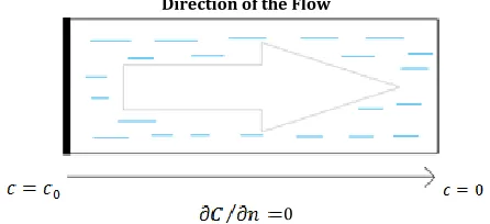
The equation for the transmission of a pollutant in an assumed aquifer is studied in one dimension, as shown in Fig. 1. The contaminant source is considered as a continuous point. In this case, the flow is considered uniform and along the x-axis. The concentration of pollutant t=0 in the aquifer is zero. The concentration of the pollutant in t>0 the left
border of the aquifer is C0.The boundary conditions
of this problem are as follows: Initial conditions:
(25)
Boundary conditions:
(26)
(27)
The diffusion coefficient in the horizontal
direction is equal to , and the
leakage velocity is equal to . The
range is equal to L = 100 m, and the contaminant
concentration is equal to . Boundary
condition in this problem is a combination of Dirichlet and Newman boundaries. Points are distributed at a distance of 10 meters uniformly in the range of the problem. The assumed geometry of the aquifer and the boundary conditions of the problem are indicated in Fig 1.
Direction of the Flow
0
Fig 1. Domain in the one-dimensional mode
Results
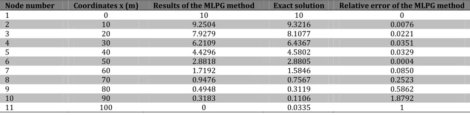
Node values were approximated using the MLPG method at different time intervals. The values of the numerical solution were compared with the calculated values of Agata's exact solution at different times (15), the results of which are presented in Fig. 2 and Table 1. It can be concluded from this comparison that the MLPG method has acceptable accuracy.
Estimation of total error
In order to estimate the total error, a function is defined in the range of study, which is then quantitatively calculated and presented (16):
(28)
Where E is the average of the error of the function,
is the exact value, is the numerical
value of the function, and n is the number of nodes. The overall estimated error is 0.03, thus indicating that the meshless method yields acceptable values.
27 J Health Sci Technol.2018 April 2(1): 23-28.
-
125
Fig 2. Comparison of numerical and exact values at time t = 300 day
Table 1. Results of the Petrov-Galerkin method in 300 days
Node number Coordinates x (m) Results of the MLPG method Exact solution Relative error of the MLPG method
1 0 10 10 0
2 10 9.2504 9.3216 0.0076
3 20 7.9279 8.1077 0.0221
4 30 6.2109 6.4367 0.0351
5 40 4.4296 4.5802 0.0329
6 50 2.8818 2.8805 0.0004
7 60 1.7192 1.5846 0.0850
8 70 0.9476 0.7567 0.2523
9 80 0.4948 0.3119 0.5862
10 90 0.3183 0.1106 1.8792
11 100 0 0.0335 1
Discussion
Figure 2 shows MLPG method and exact soltution in a graph. The correspondness of MLPG results to exact one indicates the high accuracy of MLPG in simulation of contamination transmition. This figure also confirms the boundary conditions of problem. In the first place as the boundary conditions is consistant contamination (Dirichlet), it is equal to 10m in all time steps. Table 1 presents the value of contamination which is derived from MLPG in each node in comparison of thier real value. The Mfree model shows more error in 10th node which its relative error equal to 1.87. Although in the rest of nodes the relative error is less than 1.
Conclusion
In the present circumstances, the issue of groundwater pollution is more critical for the exploitation of the limited fresh water resources than ever. Modeling this phenomenon is essential in order to understand the status quo and to predict the future status of aquifers. The advantage of this method is the lack of need for meshing of the solution range, which reduces the time it takes to perform the calculations. In this study, using the MLPG method, the modeling of the transmission of pollutants in groundwater in homogeneous mode
was investigated. For this reason, the governing equations of the problem were discretized using the Petrov-Galerkin local method, and for approximation of the shape function, moving least squares was used. The results of this method were compared with the exact results. The results of this comparison indicate the acceptable accuracy of the Petrov-Galerkin local method.
Acknowledgements
The authors express their gratitude to the Faculty of Engineering at Birjand University, Birjand, Iran for their support.
Conflicts of Interest
The authors declare no conflicts of interest.
Financial Support
The authors appreciate Birjand University for their financial support.
References
1. Ye Y, Chiogna G, Cirpka O, Grathwohl P, Rolle M. Experimental investigation of compound-specific dilution of solute plumes in saturated porous media: 2-D vs. 3-D flow-through systems. J Contam Hydrol. 2015; 172:33-47. PMID: 25462641DOI: 10.1016/j.jconhyd.2014.11.002
2. Boddula S, Eldho TI. A moving least squares based
28 J Health Sci Technol.2018 April 2(1): 23-28.
-
125
meshless local petrov-galerkin method for the simulation of contaminant transport in porous media. Eng Analysis Boundary Elements. 2017; 78:8-19. DOI: 10.1016/j. enganabound.2017.02.003
3. Gingold RA, Monaghan JJ. Smoothed particle hydrodynamics: theory and application to non-spherical stars. Mon Not R Astron Soc. 1977; 181(3):375-89. DOI: 10.1093/mnras/ 181.3.375
4. Liu GR, Gu YT. An introduction to meshfree methods and their programming. Berlin: Springer Science & Business Media; 2005.
5. Atluri SN, Zhu T. A new meshless local Petrov-Galerkin (MLPG) approach in computational mechanics. Computation Mech. 1998; 22(2):117-27. DOI: 10.1007/s004660050346 6. Long S, Atluri SN. A meshless local Petrov-Galerkin method
for solving the bending problem of a thin plate. Comp Model Eng Sci. 2002; 3(1):53-64.
7. Abbasbandy S, Shirzadi A. MLPG method for two-dimensional diffusion equation with Neumann's and non-classical boundary conditions. Appl Numer Math. 2011; 61(2):170-80. DOI: 10.1016/j.apnum.2010.09.002
8. Liu GR. Meshfree methods: moving beyond the finite element method. Florida: CRC Press; 2009.
9. Belytschko T, Gu L, Lu YY. Fracture and crack growth by element free Galerkin methods. Model Simulat Mater Sci Eng. 1994; 2(3A):519.
10.Mohtashami A, Akbarpour A, Mollazadeh M. Development of two dimensional groundwater flow simulation model using meshless method based on MLS approximation function in unconfined aquifer in transient state. J Hydroinform. 2017; 19(5):640-52. DOI: 10.2166/hydro.2017.024
11.Mohtashami A, Akbarpour A, Mollazadeh M. Modeling of groundwater flow in unconfined aquifer in steady state with meshless local Petrov-Galerkin. Modares Mech Eng. 2017; 17(2):393-403. [Persian]
12.Hamabi K, Parninneia M. Modeling of pollution transmission in groundwater of Nayband National Park. 13th Iranian Hydraulic Conference, Tabriz, Iran; 2014. [Persian] 13.Freeze RA, Cherry JA. Physical properties and principles.
Englewood Cliffs, NJ, USA: Groundwater, Prentice-Hall Inc; 1979.
14.Afshar MH. Approximation process and finite element method. Tehran: Iran University of Science and Technology Publishing; 1996. [Persian]
15.Ogata A, Banks RB. A solution of the differential equation of longitudinal dispersion in porous media: fluid movement in earth materials. Washington, D.C.: US Government Printing Office; 1961.
16.Darvishinejad N, Barani G. Application of meshless local Petrov-Galerkin (MLPG) method to modeling the water leakage from the dam. 11th National Seminar on Irrigation and Evapotranspiration, Kerman, Iran; 2011. [Persian]