Abstract—By applying the direct boundary element technique for solving the problem of the 2D compressible fluid flow around obstacles a singular boundary integral equation, formulated in velocity vector terms, arises. A boundary element method with quadratic boundary elements of lagrangean type is developed in this paper in order to solve this singular boundary integral equation. The integral representation of the velocity is reduced by discretization to an algebraic system. All coefficients depend only on the nodes coordinates used for the boundary discretization so it can be easily implemented into a computer code, in order to get the numerical solution of the problem to be solved. We test the method solving a particular case in which the problem has an analytical solution. Comparing the values of the exact solution with the calculated ones we remark a high degree of accuracy.
Index Terms— direct boundary element method, singular integral equation, compressible fluid flow, quadratic boundary element.
I. INTRODUCTION
When solving problems of fluid flows around different kinds of obstacles, and in general boundary value problems for systems of partial differential equations, which imply the presence of an unbounded domain, a very efficient method which can be used is the boundary element method (BEM) ([1],[2],[3]).
When applying this method there is no need to introduce a fictive boundary at great distances as in case of using other methods as finite differences, or finite element method, and also there is no need to make a mesh of the whole domain involved in the problem because BEM has the ability to reduce the problem dimension by one. Because only the boundary of the domain must be discretized the problems are reduced to systems of linear equations much smaller than in other cases. As a consequence the computational efficiency is improved by applying this method.
To achieve this reduction of dimension it is necessary to formulate the problem as a boundary integral equation, which is usually a singular one. Two techniques can be used to obtain the boundary formulation of the problem: the direct and the indirect technique(see [2],[3]).
Manuscript received March 23, 2010.
Ion Vladimirescu is with the University of Craiova, Faculty of Mathematics.
Luminita Grecu is with the University of Craiova, Faculty of Engineering and Management of Technological Systems Dr. Tr. Severin, (phone:+40252333431; fax: +40252-317219; e-mail: lumigrecu@ hotmail.com).
In this paper we use higher order boundary elements to solve the singular integral equation resulting as an application of the direct integral technique to the bi-dimensional problem of subsonic compressible fluid flow around obstacles.
Different types of numerical methods, have been applied by other authors (finite differences, finite elements, Galerkin collocation methods, and other techniques) to solve problems of fluid flow around obstacles. The BEM was used as well but some authors have considered the incompressible case only([4]), and mostly have used the potential or stream function as initial unknowns of the problem. The velocity and pressure fields were deduced through a differentiation technique after finding the potential or stream function. In this approach the singular boundary integral equation to solve is obtained in velocity vector terms, so we find the perturbation velocity, without any differentiation. Therefore the errors which arise are expected to be smaller than in other cases.
Using higher order boundary elements, we ensure a global continuity for the unknown function and a better approximation for it and for the geometry of the problem than in case of using a collocation method to solve the boundary integrals ([5], [7]), constant (see[8]) or linear boundary elements (as in [9]).
II. THE SINGULAR BOUNDARY INTEGRAL EQUATION -DIRECT TECHINQUE
We consider that a uniform, steady, potential motion of an ideal inviscid fluid of subsonic velocity
U
i
, pressure
p
and density
is perturbed by the presence of a fixed body of a known boundary , noted C, assumed to be smooth and closed. We want to find out the perturbed motion, and the fluid action on the body.Introducing dimensionless variables V and p, through relations:
i
V
p
p
U
p
U
V
21
1
,
we have:
0
,
0
2
Y
U
X
V
Y
V
X
U
(1)The boundary condition is:
1U
NXVNY 0, (2)where N is the normal unit vector outward the fluid (inward the body).
Because it is also required that the perturbation velocity vanishes at infinity we deduce relation: p = - U.
A Direct BEM with Higher Order Boundary
Elements for the Compressible Fluid Flow
around Smooth Obstacles
For xX ,y
Y,u
U,vV , the system of equations becomes:
0
0
y
u
x
v
y
v
x
u
(3)
the boundary condition:
u
n
x
2vn
y
0
on
C
, (4) andlim
,
0
u
v
,where
n
0x,
n
0y are the components of the normal unit vector outward the fluid (inward the body) in the point0
x
, 1M2(for the subsonic flow, M= Mach numberfor the unperturbed uniform motion).
Using a direct boundary element method integral representations for the components of velocity in the fluid domain,
, are first obtained,u
,
v
,
(seee[5]). Considering
x
0
C
the perturbation velocity in any point of the boundary is obtained:
C
x y
C
y x
ds x n x x v x n x x u x v
ds x n x x v x n x x u x u x u
0 * 0
*
0 * 0
* 0
, ,
, ,
2 1
C
y x
C
y x
ds x n x x v x n x x u x v
ds x n x x u x n x x v x u x v
0 * 0
*
0 * 0
* 0
, ,
, ,
2 1
(5) where
n
0
n
x
0 ,u
*,
v
*are the fundamental solutions given by the following relations ( see[6]):
20 2
0 0 0
*
2 0 2
0 0 0
*
2 1 ,
, 2
1 ,
y y x x
y y x
x v
y y x x
x x x
x u
(6)
Denoting
G
u
n
y
vn
x, and supposing that G is a holderian function on C, we get the representations:
C x y
y x
Gds u n n
n n M v x
u *
2 2 2 2 * /
0 2
C x y
y x
Gds
v
n
n
n
n
M
u
x
v
*2 2 2 2 * / 0
2
(7)and the singular integral equation:
* 0 * 0
0 22 2 2 /
0 * 0 * / 0
2 2
2
y C
y x y x
y x C
y x
n Gds n u n v n n
n n M
ds G n v n u x
G
(8)
The sign “′ “denotes the principal value in Cauchy sense of the integral (see[10]).
III. SOLVING THE SINGULAR BOUNDARY INTEGRAL
EQUATION WITH QUADRATIC ISOPARAMETRIC BOUNDARY ELEMENTS
In [8] the boundary integral equation is solved by using a constant boundary elements, and in paper [9] linear boundary elements are used.
In the herein approach we consider quadratic isoparametric boundary elements for solving equation (8). Same kind of boundary elements were used in paper [11], but for solving the singular integral equation obtained by an indirect method with sources distribution on the boundary, for the same problem.
So we consider that the boundary is divided into N one-dimensional quadratic boundary elements, noted
L
i, each of them with three nodes: two extreme nodes and an interior one. The extremes of the segmentL
i are notedi i i
x
x
x
1,
2,
3, in a local numbering. We have the relations:1
,
1
,
3 1
1
x
i
N
x
i i , and 11 3
x
x
N
contour C being closed.We obtain the discrete form of equation (8):
* 0 * 0
02 2 2 2
1
0 * 0 *
1 0
2 1
y L
y x
y x
y x N
i
L
y x
N
i
n Gds n u n v n n
n n M
ds G n v n u x
G
i
i
(9) Considering that equation (9) is satisfied in every node (
x
0
x
j), we obtain:
j y
L L
j y j
x N
i
L L
j y j
x N
i j
n Gds u n Gds v n M
ds G v n Gds u n x
G
i i
i i
* *
1 2
* *
1
2 1
(10)
where
n
xj,
n
yj are the components ofn
j
n
x
j , and2 2 2
y x
y x
n
n
n
n
.For describing the geometry and the behavior of the unknown
f
, on a boundary element, we use a quadratic model, with the same set of basic functions, noted3 2 1
,
N
,
N
N
x
ix
,y
N
y
i ,G
N
G
i (11) where
N
is a matrix with a single line,
N
N
1N
2N
3
,
,
1,1 21 ,
1 ,
2 1
3 2 2
1
N N
N
xi , yi the column matrices made with the coordinates ofthe nodes of element
L
i, and
G
i the column matrix made with the nodal values of the unknown function G onL
i,
i i i i
tG
G
G
G
1 2 3 .There are used two systems of notation: a global and a local one (global-
G
i is the value of G for the node number i,i
1
,
2
N
-and local-G
li,
l
1
,
3
,
i
1
,
N
is the value for the node number l of element i).Introducing in equation (10) the considered approximation models, and doing some calculus we get:
N i
i j
i j i j
y N i
i j
i j i j
x j
d J G N x x N
y y N n
d J G N x x N
x x N n
x G
1 1
1 2
1 1
1 2
N i
i j
i j i j
x N G J d
x x N
y y N n
M 1
1
1 2
2
jy N i
i j
i j i j
y
n
d J G N x x N
x x N n
M
2 1
1
1 2
2
(12) Further we obtain a simple form of the above equation:
j y N
i l l ij l i j
y
N
i l l ij l i j
x N
i l l ij l i j
n C
G n
M
B G n
M a G x
G
2
1 3
1 2
1 3
1 2
1 3
1
(13)
Denoting by:
i i i
i
x
x
x
m
1
3
2
2,n
i
x
3i
x
1i,u
ij
x
2i
x
j,i i i
i
y
y
y
M
1
3
2
2,N
i
y
3i
y
1i,U
ij
y
i2
y
j, 42 2
i i i
M m a
4 2 2
i i i
N n
aa
2 i i i i i
N M n m
b ,
ij i ij i i
ij
aa
m
u
M
U
c
,d
ij
n
iu
ij
N
iU
ij, 22
ij ij ij
u
U
e
,i
,
j
1
,
2
N
a
ib
iaa
iJ
4
2
2
, (14)we get:
ij ijnot
ij ij ij
i i j i
N
N
e
d
c
b
a
x
x
N
4 3 22
Then, denoting by
,
,
1
,
2
,
0
,
1
,
2
,
3
,
4
1
1
k
N
j
i
d
J
N
I
ij k k
ij
, (15)we obtain the following expressions for the first coefficients in (13):
4 3
1
4
4 ij
j y i i j x i i ij j y i j x i
ij I
n M N n m n I n M n m a
2 12 4
2 2
ij j y ij j x ij ij j y i ij j
x i ij
I n U n u I n N U n n
u
4 3 1
2
2
2 ij ij
j y i j x i ij j y i j x i
ij I I
n N n n I n M n m a
2
04
2
2
ij j y ij j x ij ij j y i ij j
x i ij
I
n
U
n
u
I
n
M
U
n
m
u
4 3
3
4
4 ij
j y i i j x i i ij j y i j x i
ij I
n M N n m n I n M n m a
2 12 4
2 2
ij j y ij j x ij ij j y i ij j x i ij
I n U n u I n N U n n
u
(16) In order to be able to evaluate the coefficients
B
ijl,
C
ijl we need to deduce expression of
2 2 2y x
y x
n
n
n
n
onelement
L
i, where we havex
N
x
i .By differentiating this relation we obtain the tangent field on the geometric support of the boundary element, and, taking into account the sense we have considered on the boundary we deduce that
ix
y
d
dN
n
, and
i
y
x
d
dN
n
onL
i. (17)We get the following expressions:
2
i i x
N
M
n
,2
i i y
n
m
n
(18)We obtain:
i i i i
Nm
s
r
p
where pi 4miMi ri2
miNiniMi
si niNi
2 2 2 2 2 2 2 4 4 i i i i i i i i not i n N n m N M m M Nm Evaluating the last two terms in equation (12) we deduce:
3 1 1 1 3 1 * l l ij l i l ij j i l l i L C G d J N N x x N G Gds u i where
3 4 5 6 1 4 2 2 4 2 4 4 ij i ij i i i i ij i ij i i i i i i ij i ij i i i i i ij i i ij T p u m n s n u r T m s m n r n u p T m r m n p T m p C
2 12 4 2 2 ij ij i ij ij i i ij i T u s T u r n u s
2 1 03 4 5 6 2 2 2 4 2 2 2 2 2 2 2 2 ij ij i ij ij i i i ij i i ij i ij i i ij i i i i ij i i ij i i i i i ij i ij i i i i ij i i ij T u s T u r n s T n r u p u m s T n p n s u m r T m s n r m u p T m r n p T m p C
2 13 4 5 6 3 2 4 2 2 4 2 2 4 2 4 4 ij ij i ij ij i i ij i ij i ij i i i i ij i ij i i i i i i ij i ij i i i i i ij i i ij T u s T u r n u s T p u m n s n u r T m s m n r n u p T m r m n p T m p C with
, , 1,2 , 0,...,6 1 1
k N j i d J N Nm T ij i k kij
(20) Analogous we have:
3 1 1 1 3 1 1 1 * l l ij l i l ij j i l l i L i ij j i B G d J N N y y N G d J G N N y y N Gds v i
with
2 13 4 5 6 1 2 4 2 2 4 2 2 4 2 4 4 ij ij i ij ij i i ij i ij i ij i i i i ij i ij i i i i i i ij i ij i i i i i ij i i ij T U s T U r N U s T p U M N s N U r T M s M N r N U p T M r M N p T M p B
2 1 03 4 5 6 2 2 2 4 2 2 2 2 2 2 2 2 ij ij i ij ij i i i ij i i ij i ij i i ij i i i i ij i i ij i i i i i ij i ij i i i i ij i i ij T U s T U r N s T N r U p U M s T N p N s U M r T M s N r M U p T M r N p T M p B
2 13 4 5 6 3 2 4 2 2 4 2 2 4 2 4 4 ij ij i ij ij i i ij i ij i ij i i i i ij i ij i i i i i i ij i ij i i i i i ij i i ij T U s T U r N U s T p U M N s N U r T M s M N r N U p T M r M N p T M p B (21) Denoting by
b
ijl
M
2
n
xjB
ijl
n
yjC
ijl
we can write equation (13) in a simple form:
jy N i l l ij l i N i l l ij l i
j G a G b n
x G
2 1 3 1 1 3 1
(22)By denoting
A
ijl
a
ijl
b
ijl ,i
,
j
1
,
N
l
1
,
3
equation (22) can be written as:
jy N i l l ij l i
j
G
A
n
x
G
2
1 3 1
(23) The above equation is satisfied in every node which we have chosen for the boundary discretization, so we obtain a system of linear equationsReturning to the global system of notation, we obtain the following linear algebraic system:
NN
R
G
B
R
M
A
B
G
A
,
2,
,
2
B
j
2
n
yj. (24)
G
being the column matrix made with the nodal values of the unknown functionFor that we consider the following schematic representation for the nodes used at the discretization.
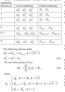
Table I Correspondence between local and global numbering
Element nr. Local numbering Global numbering
1 3
1 2 1 1
1
G
G
G
G
1G
22 3
2 2 2 1
2
G
G
G
G
3G
43 3
3 2 3 1
3
G
G
G
G
5G
6… … …
k 1 2 3
k k
k
G
G
G
G
2k1G
2kk+1 3
1 2
1 1
1
k k
k
G
G
G
G
2 k11G
2 k1… … …
N 1 2 3
N N
N
G
G
G
G
2N1G
2NThe following relations hold:
1
,
1
,
1 2 1
1
3
G
k
N
G
G
k k k1 1 1
3
G
G
G
N
(25) We can write system (23) as:j N
i ji i
j
A
G
B
G
2
1
, (26) where
1
,
1
,
1
,
1
2
,
,
1
,
2
,
3 1 1
3 1
1 2
i
if
A
A
N
k
k
i
if
A
A
N
k
k
i
if
A
A
Nj j
kj j k kj
ji
(27) and further we get the final form (24).
The expressions of components of matrix A in (24) are:
j
i
A
j
i
A
A
jj ji ji
,
,
(28)Solving system (24) we find the nodal values of function G. After finding
G
i the velocity components can be found with the following relations:
0 2 2
0 20 2
i y i
x
i i y i
x n x
n
G x n u
, 2
0
2 2
00
i y i
x
i i x i
x n x
n
G x n v
.
(29)
IV. NUMERICAL RESULTS
The calculation of the matrix coefficients requires several evaluations of integrals with singular and non-singular kernels. These integrals can be calculated numerically with a computer but some of them are singular. For the singular integrals ordinary rules can’t be applied so for dealing with them we must use special formulas or techniques. Some of
them are presented in papers [11], [12], [13]. The use of any of them makes possible the implementation of the method exposed into a computer code to get the numerical solution.
As shown in paper [12] the best method that can be used to treat the singularities which arise in such problems is the regularization method, which we apply it in this case too.
Even the expressions of the coefficients are a little bit complicated they depend only on the nodes chosen for the boundary discretization, so they can be computed using a computer.
The components of the velocity on the boundary are used to evaluate the local pressure coefficient with relation:
1 1
1 2
1 1
2 2 1
2 2
2
v
u M
M
Cp (30)
if
M
0
, or in case of an incompressible fluid flow with relation:u v u
Cp 2 22
.
The effectiveness and the efficiency of the method proposed in this paper is shown through an analytical checking, by making a computer code in MATHCAD which is used to obtain numerical results for particular cases which have exact solutions.
For an incompressible ideal fluid flow (
1
) and a circular obstacle the analytical expressions for the dimensionless components of the velocity and the local pressure coefficient are given by the following relations, see [6]:ucos2 ,vsin2
,
cp12cos2.
We use the computer code to get the numerical solution in this particular case. We have chosen 32 nodes for the boundary discretization.
The numerical results are presented in Fig 1, where the analytical solution is represented as well.
As we can see the error between the numerical and the exact solution is very small.
cp
-3.500 -3.000 -2.500 -2.000 -1.500 -1.000 -0.500 0.000 0.500 1.000 1.500
1 3 5 7 9 11 13 15 17 19 21 23 25 27 29 31
[image:5.595.308.547.580.716.2]num exact
V. CONCLUSIONS AND FURTHER WORK
The Direct Boundary Element Method (BEM) is an efficient numerical technique, which offers good numerical results when solving problems of 2D compressible fluid flow around obstacles, especially when higher order boundary elements are used. Even when using a small number of nodes for the boundary discretization the numerical results are of great accuracy if suitable methods for the treatment of the singularities are used. As one can sees the errors are indeed very small, fact that shows the efficiency of the method.
Comparisons between the exact solution and the numerical solutions obtained when solving the singular integral equation with constant, linear and quadratic boundary elements can also be performed, as well as a comparison between the exact solution, the numerical one obtained when an indirect technique with sources distribution and quadratic boundary elements is used. This comparison will establish which method offers better results in case of smooth obstacle. Even if the boundary equation is more complicated than the singular boundary integrals obtained when applying the indirect techniques, the direct boundary method can successfully be used in case of profiles with cusped trailing edge, because it can handles easier with the Kutta-Jukovsky condition.
REFERENCES
[1] Aliabadi M.H., Brebbia C.A., „Advanced formulations in boundary element methods, Computational Mechanics Publications”, Elsevier Applied Science, 1993
[2] Brebbia, C.A., Walker, S., Boundary Element Techniques in Engineering, Butterworths, London, 1980.
[3] Brebbia, C.A., Telles, J.C.F., Wobel, L.C., Boundary Element Theory and Application in Engineering, Springer-Verlag, Berlin,1984 [4] Carabineanu A.: „A boundary element approach to the 2D potential
flow problem around airfoils with cusped trailing edge”, Computer Methods in Applied. Mechanics and Engineering. 129(1996) [5] Dagoş, L., Metode Matematice în Aerodinamică (Mathematical
Methods in Aerodinamics), Editura Academiei Române, Bucureşti, 2000.
[6] Dragoş, L., Mecanica Fluidelor Vol.1 Teoria Generală Fluidul Ideal Incompresibil (Fluid Mechanics Vol.1. General Theory The Ideal Incompressible Fluid), Editura Academiei Române, Bucureşti, 1999. [7] Dragoş L., Dinu A., A direct Boundary Integral Equations Methods to
subsonic flow with circulation past thin airfoils in ground effect, Comput. Methods Appl. Mech. Engrg., 121(1995)163.
[8] Grecu, L., Demian G., Demian M.: “Two boundary element approaches for the compressible fluid flow around a non-lifting body” U.P.B Sci Bull. Series A, Vol.71, Iss.1, 2009
[9] Grecu, L., "A Boundary Element Approach for the Compressible flow Around Obstacles", Acta Universitatis Apulensis, Mathematics-Informatics, No 15/2008, pag 195-213.
[10] Lifanov, I. K., Singular integral equations and discrete vortices, VSP, Utrecht, TheNetherlands, 1996.
[11] I. Vladimirescu, L. Grecu, „An Efficient Technique to Treat Singularities when Applying BEM with Quadratic Boundary Elements to the Problem of Compressible Fluid Flow”, Lecture Notes in Engineering and Computer Science: Proceedings of The 2009 International Conference of Applied and Engineering Mathematics, ICAEM 2009, 1-3 July, 2009, London, pp 984-988.