A PSO-BASED NEURAL NETWORK ENSEMBLE WITH THE
APPLICATION OF FLAME COMBUSTION DIAGNOSIS
1LI DESHENG, 2HE QIAN
1Dr, School of Science, Anhui Science and Technology University, China
2
Associate Prof, School of Information& Communication, Guilin University of Electronic Technology,
China
E-mail: [email protected] , [email protected]
ABSTRACT
In thermal power station, pulverized coal furnace is widely used. It requires the chamber of furnace holding steady uniform flame, and ensureing that strong full combustion. This study has developed a neural network ensemble model to perform the judgement of combustion diagnosis based on the spectral distribution of the light intensity pulse signal of the flame. Compared with the single neural network, the two-stage integrated model of neural network ensemble, based on Bootstrap and electoral cooperative particle swarm optimization, can found the internal relations among inputs and outputs according to the learning of internal rules, and weaken the human factors in the weights determination. Based on the experiments on real scenario, the results show that the proposed model outperforms all the compared ones in perspective of the convergence speed of total error, and also obtains stable classification effect.
Keywords: Particle Swarm Optimization (PSO), Swarm Intelligence (SI), Artifical Neural Network Ensembles (ANNE), Flame Combustion Diagnosis
1. INTRODUCTION
In China, the thermal power station units used pulverized coal furnace is in the majority. It requires the chamber of furnace holding steady uniform flame, and ensures that strong full combustion [1]. If combustion is not full or unstable, it not only reduces the boiler thermal efficiency, but also produces pollution waste and noise, or even cause furnace explosion accident in some extreme cases. Therefore, effective fire inspection and combustion diagnosis device must be deployed on the furnace.
The main fuel of furnace in thermal power station includes coal, oil and gas, both of which can emit ultraviolet, visible light, and infrared in the combustion process. The characteristics of different fuel combustion characteristics are also not identical. In our research, the flame combustion diagnosis of pulverized coal furnace is only considered with the following traits in the traditional detection observation.
● When pulverized coal with the wind spurts from the injector, the temperature of pulverized coal is low not reaching to the ignition point and not yet combust. From the perspective of field
experimentation, it can be seen that a strap-shaped dark mixture of coal and wind spurted from the inflamer.
● Then pulverized coal is heated by the High temperature radiation and flame reflux in the furnace. After that, the coal begins the thermal decomposition reaction, resolves the volatilization powder, and combusts strongly. Because at this time the combustion is mainly caused by the volatile powder and a small amount of coke particle, so the luminance is not reaching the maximum but with the maximal flame combustion frequency. This trait is the judgment basis of the traditional detection way.
● Pulverized coal particles goes further furnace and the resolved volatilization powders has burn off basically. The coal begins to combust strongly and produces a lot of heat. Then the temperature and luminance of the flame reaches the maximum.
● After the most of coal particles burn off, only a few large particles continue to burn and form high temperature air. Accordingly, brightness and flicker frequency of the flame reduce.
characteristic of pulverized coal flame radiation light is the flame pulsation varying with time sequence. According to literature [2], it is difficult to distinguish the case of stable and unstable combustion only from the flame radiation intensity time series shown in Fig.1, but the it makes a explicit distinction on the spectral distribution. As illustrated in Fig.2, we can see that in case of stable combustion, amplitude values of low frequency component power spectrum are larger than those of high frequency component.
Fig.1 Time Sequence Of Stable Combustion.
Fig.2 Spectral Distribution Of Stable Combustion.
Based on this characteristic, we can acquire the light intensity pulse signal of the flame, and perform effectively pattern recognition on the case of stable, unstable and uncertain combustion through wavelet transform processing and the training of neural network ensemble. Then the final judgment of combustion diagnosis can be drawn based on this approach.
2. ECPSO ALGORITHM
PSO algorithm was first introduced by Kennedy and Eberhart [3] as a simulation of this behavior, but quickly evolved into one of the most powerful optimization algorithms in the computational intelligence field. The algorithm consists of a population of particles that are flown through an n -dimensional search space.
The position of each particle represents a potential solution to the optimization problem and is used in determining the fitness (or performance) of a particle. In each generation of iteration, particle in swarm can be updated by the values of the best solution found by it and the one found by the whole swarm by far according to the following equation set (1):
1
2
() ( )
() ( )
new best
id id id id
best
gid id
new new
id id id
V V C Rand P P
C Rand P P
P P V
ω
= × + × × −
+ × × −
= +
(1)
where:
V
idnew – particle’s new movement distance ina step, limited to [vmin, vmax], Vid – particle’s
current movement distance in a step, Pidnew –
particle’s new position, Pid – particle’s current
position, Pidbest – Pid’s best experience f,
best
gid
P –
gid-th particle’s best experience, Vid – particle’s current
movement distance in a step, ω– inertial weight
factor, C1 – cognition learning factor, C2 – social
learning factor.
Another variation of PSO, Cooperative Multi-Swarm Particle Multi-Swarm Optimization (CMPSO) proposed by Van den Bergh F.[4] could be seen as a improvement to the single swarm PSO, in which the high-dimension search space can be decompose into small scale ones similar to the idea of RELAX/CLEAN algorithm. However, its difference to it is that due to the imported information exchange mechanism among particles, the more accurate estimates did not need reduplicative iterations any more. Compared to basic single swarm PSO, both robustness and precision are improved and guarantied.
In key idea of CPSO is to divide all the n -dimension vectors into k sub-swarms. So the front
n/k swarms are ⌈n/k⌉-dimensional, and the k−(n/k)
swarms behind have ⌊n/k⌋-dimensional vectors. In each pass of iteration, the solution is updated based on k sub-swarms rather than the original one. When
0 25 50 75 100 125 150 175 200 225 250 0
0.2 0.4 0.6 0.8 1.0 1.2 1.4 1.6
0 1000 2000 3000 4000 5000 6000 7000 8000 9000 10000 0.26
the particles in one sub-swarm complete a search along some component, their latest best position will be combined with other sub-swarms to generate a whole solution. The function b performs exactly this: it takes the best particle from each of the other sub-swarms, concatenates them, splicing in the current particle from the current sub-swarm j
in the appropriate position. Particles in each sub-swarm update their latest best positions according to Formula (3), while the latest best positions of each sub-swarm are renovated by Equation (4), where Si denotes the i-th sub-swarm. Note that
Equation (2) is the composition function of position with the global best fitness of all sub-swarms which is also illustrated in Fig. 1.
1 1 1
( , ) ( . ,..., . , , . ,..., . ),
1
best best best best
gid u gid u gid k gid
b u Z S P S P Z S P S P u k
− +
=
≤ ≤
(2)
( , . ) ( ( , . ), ( , . )),
1
best best
u id u id u id
b u S P argmin fitness b u S P b u S P u k
=
≤ ≤
(3)
( , . ) ( ( , . )),
1 ,1
best
u gid u id
b u S P argmin fitness b u S P
id s u k
=
≤ ≤ ≤ ≤
(4)
In this paper, we use our previous cooperative swarm optimization algorithm named CMPSO-EM [5,6]. Firstly, we will discuss the dynamics of particles in the swarm, which is different with plain PSO and conventional cooperative PSO algorithms. The movement equation can be formalized as following equation set (5):
1
2 3
() ( )
ˆ
() ( ) () ( )
new best
id id id id
best best
gid id egid id id
new new
id id id
V V C Rand P P
C Rand P P C Rand P P P P V
ω
= × + × × − +
× × − + × × ↑ −
= +
(5)
The principle of electoral cooperative mechanism is depicted in Fig.3, in which it can clearly seen that three parts: the local best position (particles with orange color), the global best position in sub-swarm (particles with blue color), and that of electoral swarm (particles with purple color) both take participate in the evaluation of fitness function with its own position. Note that the members of electoral swarm are voted from the primitive sub-swarms with dynamic population during generation of iteration.
To import this electoral mechanism into PSO, we introduce two components of it. One is Pˆegidbest, which denote the egid-th particle’s best experience, i.e., the best experience of electoral swarm. However, as the position is the one of each dimension, this component could not be used directly. So another operation ↑id is also employed to calculate the projection of Pˆegidbest, i.e., Pˆegidbest ↑id.
The function b shown in Equation (2) performs exactly this: it takes the best particle from each of the other sub-swarms, concatenates them, splicing in the current particle from the current sub-swarm j
in the appropriate position. According to this function, the composition of best
id
P , Pgidbest and
ˆbest egid
P can be calculated based on Equation (6).
ˆ
( , . ) ( ( , . ), ( , . )),
1 ,1
best best best
u gid u id gid
b u S P argmin fitness b u S P b u ES P id s u k
=
≤ ≤ ≤ ≤
(6)
Swarm-farm-1
Electral Swarm
sub-swarm-11 sub-swarm-1,n/k
Swarm-farm-s
sub-swarm-s1 sub-swarms,n/k
ˆbest egid
P
best gid
P
best id
P
...
... id
V
Fig.3. Principle Of Electoral Cooperative Mechanism
Fig.4. Landscapes Of Test Functions
Fig.5. Particle Trajectory İn ECPSO And PSO
3. NEURAL NETWORK ENSEMBLE
BASED ON ECPSO AND BOOTSTRAP
According to literature [7,8], the definition of NNE is depicted as: Neural network ensemble (called NNE) is a limited set of integrated neural networks to learn on the same question, whose output is also integrated and determined by the outputs of individual networks.
The model of neural network ensemble proposed in this paper can be divided into two stages: the first stage includes T individual network which is trained by the training set generated by bootstrap technique. In the second stage, the output of neural network ensemble is obtained by the weighted summation of the networks in the first stage. Moreover, these combined weights are optimized by ECPSO based on performance on the validation set. Finally, the output of the whole model is the simple average of the second stage’s outputs.
Bootstrap is an improvement on cross-validation offering better estimation of generalization error. Let the training pairs from the observed data set D be Z x yi( ,i i)(i=1, 2,...,N). The
basic idea behind bootstrap is to create a number of data sets, each of the same size of the original training set, by random sampling with replacement from the original train set. By sampling B times, B
bootstrap data sets are created. Each of bootstrap data set is used separately to re-train the network and verify its fitness by repeating experiments B
times. There are many ways to estimate generalization error when using bootstrap.
One approach is to train the network using bootstrap data sets and compute its error on the training set. Let ˆ ( )*b
i
f x be the predicted output for
i
x based on the neural network trained from the b -th bootstrap data set. The estimated generalization error is as follows:
*
1 1
1 1 ˆ
ˆ B N ( , b( ))
boot i i
b i
E L y f x
B N = =
=
∑∑
(7)This would be an underestimation of the true error because of the considerable overlap between the bootstrap training set and the original training set. A better estimation can be obtained by using the idea of cross validation: a single observation as the validation data and the remaining observations from the sample as the training data, as is done in leave-one-out bootstrap and 0.632 estimator bootstrap.
The advantage of using bootstrap is that it not only offers an estimation of generalization error, but also the confidence intervals for network output, which can be used for aggregating neural networks. For example, in the bagging algorithm, each bootstrap training set is used to train a neural network, the output of which can then be aggregated.
In this paper, one effective way of creating distinct neural networks is to train them using different data sets. The bootstrap resampling used in Bagging is quite effective. Let the original training set be D={(x yn, n),n=1,..., }N . By
resampling from it, a new data set
t
D of the same size is created, which can then be used to train the t-th neural network. Since neural network is an unstable learner in the sense that it suffers from fluctuations due to initial weights and data set, an aggregation of neural networks based on Bagging provides better generalization capabilities. TBPSOEN, for example, uses boostrap to create
different data sets for training distinct individual neural networks.
The PSO algorithm has two advantages in the optimization of output weights for neural network aggregation. Firstly, numerical iteration is employed in its solving process. Since no matrix inversion is involved, the cases where the weights deviate from their true values due to ill-conditioned matrixes can therefore be avoided. Secondly, it uses real coding where the combination of weights can be directly used as particles' code. In this way, by imposing constraint on the optimization scope of the particles, the weights are also constrained in the optimization process. Given T trained neural networks h h1, 2,...,hT , here is how to optimize
weights
α α α
( 1, 2,...,α
T)
by using ECPSO
algorithm as shown in Algorithm 1.
Algorithm 1 ECPSO-CompoWeight-Opt
Step 1. Input the data for composite weight optimization: V x y x( , ( ))(i i i=1, 2,...,M).
Step 2. Given the population p , maximal
generation of iteration imax, maximal velocity, and
the optimal range [
α α
lb, ub].Step 3 For each subswarm do Step 4 to Step 7. Step 4. iw=1, each particle is encoded as a
1×T vector
1 2 : ( , ,..., T)
α α α α
α
.Step 5. Calculate the fitness function F =1 /Rw,
where 2
1 1
1
( ( ) ( ))
M T
w i t i i
i i
R y x h x PE
M = =
α
=
∑
−∑
+ is theobjective function for optimization;
2
1 ( 1)
T t i i
PE n
α
=
= ⋅
∑
− is the penalty function item tolimite the weight sum to 1, n is a big positive number.
Step 6. Update the position and velocity of particles.
Step 7. 1
w w
i = +i . If 1
w w
i ≤i + , return Step 4. Step 8: (Electoral procedure). Get the votes of primitive sub-swarms, and elect the best (first time randomly) particles in respective primitive sub-swarms into a new electoral swarm.
Step 10. Suppose that the optimal particle is o
P ,
after normalized processing, the corresponding composite weight is o( 1o, 2o,..., o)
T
α α α
α
; while therelated output of the NNE is
1
( ) ( )
T o t t t
h x
α
h x=
=
∑
.4. EXPERIMENTAL RESULTS
As bootstrap is used in the training, the number of data included in
t
D which are not in D is
1
(1 ) |N | 0.368 | |
D D
N
− ≈ , i.e., about 1/3 of data of
D not appear in
t
D . Each individual neural network only used part of data in D, so when data set on a smaller scale, D can used as validation set
V , which is deployed to estimate the neural network ensemble without another additional validation set. In practice, even in the case of
individual network for prediction, it is regular to choose samples with optimal performance in V .
According to the above method, the sample data are divided into two groups randomly: One group with 50 samples is used for training and verification; while another 50 for prediction. The data are performed for 50 times and the result is the average value of them.
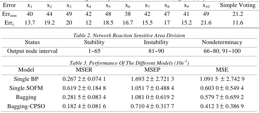
[image:6.612.94.519.327.514.2]The samples for network training come from the CCD camera’s image signals of a 250MW furnace in a thermal power station. We choose 4 typical flame images corresponding to the cases of full stable, low critical, and unstable combustion. The related output expectations are divided into intervals (0.7,1), (0.25,0.7) and (0,0.25). Table 1 illustrates the error percentage of of individual network in fist stage NNE, while table 2 shows the network reaction sensitive area division recognized by the NNE.
Table 1. Testing Result Of Individual Network In Fist Stage NNE (%)
Error x1 x2 x3 x4 x5 x6 x7 x8 x9 x10 Simple Voting
Errsum 40 44 49 42 48 38 42 47 41 49 21.2
Errc 13.7 19.2 20 12 18.5 16.7 15.5 17 15.2 21.6 11.6
Table 2. Network Reaction Sensitive Area Division
Status Stability Instability Nondeterminacy
Output node interval 1~65 81~90 66~80, 91~100
Table 3. Performance Of The Different Models (10e-3)
Model MSER MSEP MSE
Single BP 0.267 2
±
0.074 1 1.693 2±
2.721 3 1.091 5±
2.742 9Single SOFM 0.619 2
±
0.184 8 1.051 7±
0.488 4 0.603 0±
0.549 4Bagging 0.281 5
±
0.083 4 1.081 0±
0.619 2 0.579 7±
0.659 2Bagging-CPSO 0.182 4
±
0.081 6 0.710 4±
0.317 7 0.412 3±
0.386 9Based on neural network training and classification, we can see that the network for different combustion situation has obviously different reaction sensitive areas. For the combustion stability under the condition of flame signal low frequency power spectrum value input, the output network reaction sensitive area on the left is 1-65, but to combustion instability circumstances, the output network reaction sensitive area is 81-90. In addition, for the output line array division, there exist no strict rules, i.e., stable and unstable condition of the region boundary is uncertain. These areas, such as 66~80, 91~100, can be seen as the overlap region of two kinds of cases, which can't used for judging the flame stability.
Firstly, the mean square error on the training set, MSER, is defined in Eq.(2) to reflect the training accuracy of the network model. Secondly, the MSEP in Eq.(3) is also used to indicate the generalization ability of the neural network. Finally, the total error MSE is the mean square error defined on all samples.
2
1
( [ ( ) ] ) /
N
i i
i
MSER y x y N
=
=
∑
− (8)2
1
( [ ( ) ] ) /
N
i i
i
MSEP y x y P
=
=
∑
− (9)where
x
i is the input of training,y
i is the targetthe size of the training set ,while
P
is the size of the prediction set.In the experiment of our research, we establish a model of ECPSO-NNE and then compare it with other models, such as the single optimal NN, Bagging method, and GA-NNE. The prediction result MSEP of 50 running time is shown in Fig.7, and the mean and variance of corresponding MSER, MSEP, and MSE are illustrated in Table.3. Fig.7 dispicts the curves about the changes of objective function in NNE and BP. From it, it can be seen that NNE has faster convergence speed than BP.
0 50 100 150 200 250 300 350 400 450 500 6900
7000 7100 7200 7300 7400 7500
fit
nes
s
v
al
ue
evolvement generation
BP-NN ECPSO-NNE
Fig.7. Changes Of Objective Function In ECPSO-NNE And BP-NNE
From the table 3, it can be seen that the single network may cause over-fitting problem which make the prediction ability decline. By comparison, ECPSO-NNE, which need only simple design process, has obtained better modeling effect. Concretely, compared with single NN, the training error dropped 3.4%, and generalization error declined 37%; In contrast with the Bagging and GA-NNE, the generalization error descended 28.2% and 31.4% respectively. Moreover, the result is also more stable because it got the minimum variance in the 50 times experiment.
5. CONCLUSION
Compared with the single NN, the secondary integrated model of NNE, based on Bootstrap and ECPSO, can found the internal relations among inputs and outputs according to the learning of internal rules, and weaken the human factors in the weights determination. Moreover, it reduces the ‘over-fitting’ degree in data training so that it can improve the generalization capability of the model significantly. In this paper, the NNE is used to diagnose the flame combustion diagnosis of pulverized coal furnace in thermal power stations, which can help the field engineers to make the decision about the operations.
ACKNOWLEDGMENTS
This work was supported by the Natural Science Foundation of Educational Government of Anhui Province of China(No. KJ2013B073), the Science and Technology Plan Project of Chuzhou City (No.201236), and the Talent Introduction Special Fund of Anhui Science and Technology University (No.ZRC2011304).
REFRENCES:
[1] Y. Cai, “The Research of Flame Detecting and Combustion Diagnosing Based onDigital Image Processing for Coal-fired Utility Boilers”, Master Thesis, Central South University, 2003 [in Chinese]
[2] J. Ma, “Research on Flame Detection and Combustion Diagnosis Based on Spectrum Analysis and with Self Organized Neural Networks”, Power Engineering, Vol. 24, No. 6, 2004, pp. 852-856.
[3] J. Kennedy, R.C. Eberhart, “Particle swarm
optimization”, Proceedings of IEEE
International Conference on Neural Network,
1995, pp. 1942-1948.
[4] F. Van den Bergh, A.P. Engelbrecht, “Effects of swarm size on cooperative particle swarm optimizers”, Proceedings of the GECCO, 2001, 892-899.
[5] D. Li, Q. He, “A Version of Cooperative Multi-Swarm PSO Using Electoral Mechanism to Solve Hybrid Flow Shop Scheduling Problem”,
Przeglad Elektrotechniczny, Vol. 88, No. 5,
2012, pp. 22-26.
[6] D. Li, N. Deng, “An Electoral Quantum-Behaved PSO with Simulated Annealing and Gaussian Disturbance for Permutation Flow Shop Hybrid Flow Shop Scheduling Problem. Scheduling”, Journal of Information &
Computational Science, Vol. 9, 2012, pp:
2941-2949.
[7] L.K. Hansen, P. Salamon, “Nueral network ensembles”, IEEE Trans. On Pattern Analysis
and Machine Intelligence, Vol. 12, No. 10,
1990, pp. 993-1001.
[8] Sollich P, Krogh A. Learning with Ensemble: How Over-fitting can be Useful. Cambridge: