Parameter estimation and error calibration for multi-channel beam-steering SAR systems

beam-steering SAR systems

.

White Rose Research Online URL for this paper:

http://eprints.whiterose.ac.uk/148438/

Version: Published Version

Article:

Gao, H., Chen, J., Quegan, S. et al. (2 more authors) (2019) Parameter estimation and

error calibration for multi-channel beam-steering SAR systems. Remote Sensing, 11 (12).

1415. ISSN 2072-4292

https://doi.org/10.3390/rs11121415

[email protected] https://eprints.whiterose.ac.uk/ Reuse

This article is distributed under the terms of the Creative Commons Attribution (CC BY) licence. This licence allows you to distribute, remix, tweak, and build upon the work, even commercially, as long as you credit the authors for the original work. More information and the full terms of the licence here:

https://creativecommons.org/licenses/

Takedown

If you consider content in White Rose Research Online to be in breach of UK law, please notify us by

Article

Parameter Estimation and Error Calibration for

Multi-Channel Beam-Steering SAR Systems

Heli Gao1,2 , Jie Chen1,3, Shaun Quegan2 , Wei Yang1,3,* and Chunsheng Li1,3

1 _{School of Electronic and Information Engineering, Beihang University, Beijing 100191, China;}

[email protected] (H.G.); [email protected] (J.C.); [email protected] (C.L.)

2 _{School of Mathematics and Statistics, University of Sheffield, Sheffield S3 7RH, UK; [email protected]} 3 _{Collaborative Innovation Center of Geospatial Technology, Wuhan 430079, China}

* Correspondence: [email protected]; Tel.: +86-10-8233-8670

Received: 27 April 2019; Accepted: 11 June 2019; Published: 14 June 2019

Abstract:Multi-channel beam-steering synthetic aperture radar (multi-channel BS-SAR) can achieve high resolution and wide-swath observations by combining beam-steering technology and azimuth multi-channel technology. Various imaging algorithms have been proposed for multi-channel BS-SAR but the associated parameter estimation and error calibration have received little attention. This paper focuses on errors in the main parameters in multi-channel BS-SAR (the derotation rate and constant Doppler centroid) and phase inconsistency errors. These errors can significantly reduce image quality by causing coarser resolution, radiometric degradation, and appearance of ghost targets. Accurate derotation rate estimation is important to remove the spectrum aliasing caused by beam steering, and spectrum reconstruction for multi-channel sampling requires an accurate estimate of the constant Doppler centroid and phase inconsistency errors. The time shift and scaling effect of the derotation error on the azimuth spectrum are analyzed in this paper. A method to estimate the derotation rate is presented, based on time shifting, and integrated with estimation of the constant Doppler centroid. Since the Doppler histories of azimuth targets are space-variant in multi-channel BS-SAR, the conventional estimation methods of phase inconsistency errors do not work, and we present a novel method based on minimum entropy to estimate and correct these errors. Simulations validate the proposed error estimation methods.

Keywords: multi-channel; beam steering (BS); synthetic aperture radar (SAR); derotation rate; Doppler centroid; phase inconsistency errors

1. Introduction

By using azimuth antenna beam-steering technology, spaceborne synthetic aperture radar (SAR) systems can operate in beam-steering (BS) modes, such as sliding spotlight mode [1,2] and Terrain observation with progressive scan (TOPS) mode [3,4], which can achieve higher resolution or wider swaths than traditional strip-map mode. However, spaceborne SAR suffers from a conflict between azimuth resolution and range swath. By increasing the number of azimuth-receiving channels, multi-channel technology [5–7] can overcome this dichotomy and significantly increase the swath without resolution loss. As a result, multi-channel technology has been adopted in advanced spaceborne SAR systems [8–11] and processing algorithms for multi-channel strip-map imaging have been proposed, including spectrum reconstruction algorithm [12] and digital beamforming algorithm [13].

Increasing requirements for high-resolution wide-swath data are currently driving the development of multi-channel BS-SAR [14]. With the combination of beam-steering technology and multi-channel technology, multi-channel sliding spotlight SAR can provide very high resolution over a

wide swath and multi-channel TOPS can produce imaging at high resolution with ultra-wide swath. However, two main challenges that must be faced by multi-channel BS-SAR are spectrum aliasing caused by the azimuth-varying Doppler centroid and non-uniform sampling [15]. Due to the azimuth beam steering, the Doppler centroid (DC) varies linearly along targets at different azimuths [3], and can be divided into two parts: the azimuth-varying Doppler centroid and the constant Doppler centroid (CDC). The azimuth-varying Doppler centroid, whose slope is denoted as the derotation rate (DRR), is related to the illumination geometry and the beam-steering rate, while the CDC is determined by the antenna pointing direction at the central time of observation. An azimuth-varying Doppler centroid results in the azimuth bandwidth spanning several pulse repetition frequencies (PRF) and Doppler spectrum aliasing. In addition, Doppler spectrum aliasing will be much more severe in multi-channel systems because the PRF is several times smaller than in single-channel BS-SAR and the data are usually non-uniform in time.

To resolve these challenges, several imaging algorithms have been proposed [14–17], including use of sub-aperture blocking and filter reconstruction [14], a full-aperture algorithm which combines derotation and a space-time adaptive processor [16] and an approach combining derotation and filter reconstruction [15,17]. In most algorithms, however, the deration requires accurate values of the DRR and CDC to remove the spectrum aliasing. If the DRR or CDC have errors, the azimuth-varying Doppler centroid cannot be fully eliminated, resulting in inaccurate correction of the azimuth antenna pattern. In addition, for a multi-channel SAR system, phase inconsistency errors between channels are inherent. These can strongly influence the performance of multi-channel signal reconstruction and even produce ghost targets in images. In addition, amplitude inconsistency errors, timing delay errors, and channel position errors should be taken into account for multi-channel systems. Therefore, it is important to develop methods to estimate parameters and correct errors that are properly suited to multi-channel BS-SAR.

In [18], the sensitivity of the DRR to the beam-steering rate was analyzed, but its effect on imaging and its estimation were not considered. The effect of CDC error on azimuth ambiguity was analyzed in [19]. The spatial cross-correlation coefficient (SCCC) method to estimate CDC error was presented in [20] in multi-channel strip-map and involved the phase inconsistency errors, but it is sensitive to non-uniformity in the spatial sampling. For phase inconsistency errors, many estimation methods [21–29] were proposed for multi-channel strip-map SAR, mainly based on multiple signal classification (MUSIC) theory [21], but this theory is not suitable for multi-channel BS-SAR system because the noise subspace cannot be extracted from the covariance matrix of the Doppler spectrum. Adaptively Weighted Least Squares (AWLS) [27] and Doppler Spectrum Optimization (DSO) [28], which are based on the spectrum power distribution, can be exploited in multi-channel BS-SAR, but are sensitive to the CDC error. Amplitude inconsistency and timing delay errors in multi-channel BS-SAR can be easily estimated using azimuth cross-correlation [29]. The channel position errors along-track are small enough to be ignored, while the position errors in range can be integrated into the phase inconsistency errors [24].

2. Multi-Channel Beam-Steering SAR System

Azimuth multi-channel technology increases the number of azimuth-receiving channels, so significantly improves the spatial sampling rate; this is equivalent to increasing the PRF by using Digital Beam Forming technology. In addition, to achieve higher resolution or wider swath, azimuth multi-channel technology and beam-steering technology can be combined to provide new imaging modes, namely the multi-channel sliding spotlight mode and multi-channel TOPS mode.

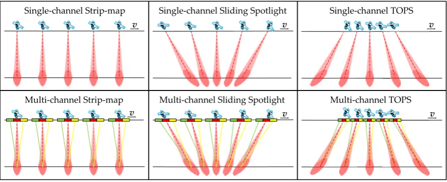
As shown in Figure 1, the beam in multi-channel sliding spotlight SAR is steered from forward-looking to backward-looking squint during an illumination period, as in single-channel sliding spotlight SAR. A target can be observed for longer than for a SAR sensor working in strip-map mode, which leads to finer resolution. TheN(N= 3 in Figure1) receivers would acquire the reflected pulse almost simultaneously, and the SAR sensor could correspondingly storeNtimes more pulse data than single-channel spotlight SAR. This means that by reducing the PRF by the factorN, the range swath could become wider while the azimuth resolution would not degrade. Similarly, multi-channel TOPS employs beam steering from backward-looking to forward-looking squint during illumination and can achieve wider swath than single-channel TOPS with the help ofNazimuth channels.

v v

v

v v

Single-channel Strip-map Single-channel Sliding Spotlight Single-channel TOPS

Multi-channel Strip-map Multi-channel Sliding Spotlight Multi-channel TOPS

v

Figure 1. The combined modes with multi-channel technology and beam-steering technology. Three different colors (green, red, and yellow) in the figure represent three different channels.

2.1. Signal Mode

A multi-channel BS-SAR system transmits a linear frequency modulated signal and each sub-channel receives the backscattered echoes. Since parameter errors in azimuth are the focus of this paper, for simplicity only the azimuth signal is considered.

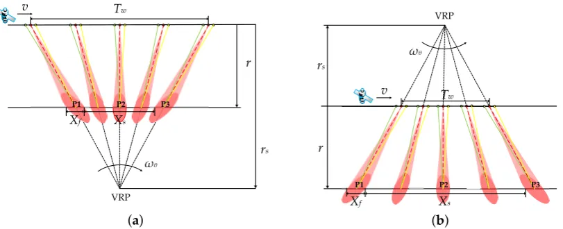
VRP

r

rs

v

W

T

Tw

Xf Xs

P3 P2 P1

(a)

VRP

v _Tw

Xf Xs

r rs

P3 P2

P1

(b)

Figure 2.Multi-channel sliding spotlight SAR and multi-channel TOPSAR. (a) is the multi-channel sliding spotlight and (b) is the multi-channel TOPSAR. Three different colors (green, red and yellow) in the figure represent three different channels.

We define a factorα(r), which multiplies the azimuth resolution in multi-channel BS-SAR due to the steering beam, as

α(r) = rs−r

rs . (1)

It can be seen that α(r) < 1 in multi-channel sliding spotlight SAR and α(r) > 1 in multi-channel TOPSAR. So, the azimuth resolution in multi-channel sliding spotlight SAR is finer than in multi-channel strip-map SAR, while coarser in multi-channel TOPSAR. Reference [15] provides another definition ofα(r), which is essentially the same.

Assuming that there areNchannels and the azimuth antenna pattern is rectangular with 3 dB beamwidth, the azimuth signal from a point target located at(r,vt0)acquired byi-th receiver can be expressed as

ss(ai)(t;r,t0) =rect "

α(r) vt+di

2

−vt0

Xf(r)

#

·rect "

vt+di

2

vTw

#

·rect

vt0

Xs

exp

−j4π

λ R

(i)_(t;r,t 0)

. (2)

In Equation (2), t is the slow time in azimuth, rect[•] represents the rectangular function, direpresents the distance between thei-th channel and the reference channel, which usually is at the center of the antenna,vis the effective velocity of the SAR sensor, andλis the wavelength.R(i)(t;r,t0)

is the instantaneous distance between thei-th equivalent phase center of the sensor and an arbitrary target, given by [17]

R(i)(t;r,t0) = 1

2R(t−t0;r) + 1 2R

t+di

v −t0;r

≈R

t+ di

2v−t0;r

+ frd

2 i

16v2, (3)

where R(t;r) = q

r2_{+ (vt)}2_{−2vtcosθ, in whichθis the aspect angle depending onr, and fr is} Doppler rate. It can be seen that the signal of thei-th channel can be seen as a replica of the reference signal-channel BS-SAR impulse response with a delay.

2.2. Spectrum Characteristics

t f

f

A

(

f

)

A(t)

t

B

a

B

a

B

a

B

s

B

t

N

·P

RF

P1

P2

P3

(a)

f

f

A

(

f

)

A(t)

t

B

a

B

a

B

a

B

s

B

t

N

·P

RF

P3

P2

P1

t

(b)

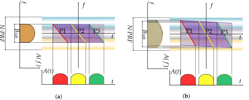
Figure 3.Time-frequency domain (TFD) diagram of multi-channel BS-SAR. (a) is for the multi-channel sliding spotlight and (b) is for the multi-channel TOPSAR. Three points are represented in red, yellow, and green. The time and bandwidth ranges are shown at the bottom and left. A(t)and

A(f)represent signal amplitudes in the time and Doppler domain, respectively. The gradient color bars (blue, grey and gold) in the background represent the total PRF that multi-channel BS-SAR can achieve withNchannels (hereN= 3). The purple area is the whole TFD of the multi-channel BS-SAR system and the shaded parts on both sides are the TFDs of edge points without full illumination.

In Figure3, three points (P1, P2 and P3) located on the left, center, and right of the azimuth are highlighted. The colored thin lines in this figure represent Doppler histories with negative slope, fr. The Doppler history of P2 is shifted upwards because of the constant Doppler centroid. The Doppler centroid of P1 is large in multi-channel sliding spotlight SAR because it experiences forward-looking squint illumination by the beam. By contrast, P3 is illuminated by backward-looking squint and has a smaller Doppler centroid. Consequently, the beam-steering results in a parallelogram TDF support which slants towards the lower right in multi-channel sliding spotlight SAR and towards the upper right in multi-channel TOPSAR. The steering bandwidth,Bs, which occurs in multi-channel BS-SAR is then given by

Bs =|kω| ·Tw, (4)

wherekω is slope of the azimuth-varying Doppler centroid (or known as derotation rate) as [3] kω =

∂ 2_λvcos(θdc(t))

∂t ≈ −

2v

λ sinθωθ≈ −

2v2_sin2_θ

λrs (5)

whereθdc(t)is the instantaneous aspect angle.

Due to the beam steering, the illumination time of any point target is expanded or shrunk by the factor 1/α(r), which results in their instantaneous bandwidth,Ba, being weighted by the same factor. Figure3shows that the instantaneous bandwidth is larger than the PRF but less thanN·PRF. The total bandwidth, including the instantaneous bandwidthBaand the steering bandwidthBsis then given by

Bt=Ba+Bs =B3dB

α(r) +|kω| ·Tw, (6)

whereB3dBis the bandwidth corresponding to the 3 dB antenna beam width.

2.3. Pre-Processing Approach

The combination of filtering reconstruction and derotation is commonly adopted to tackle spectrum aliasing in multi-channel BS-SAR because of its high efficiency and effectiveness. Derotation is essentially a convolution operation, which can be implemented by complex function multiplication and FFT, but the aliasing caused by under-sampling will remain. In the pre-processing algorithm, the FFT can be replaced by filter reconstruction, which can overcome the remaining aliasing and simultaneously produce a uniformly sampled signal.

The first phase function of pre-processing in a multi-channel BS-SAR system is given by

h(₁i)(t) =exp

(

−jπkω

t+ di

2v

2

−jπfd

t+ di

2v

+jπfrd 2 i 4v2

)

, (7)

where fdis the CDC. After multiplying by the first phase functionh( i)

1 (t), the steering bandwidthBs is eliminated and the CDC is compensated as shown in Figure4a.

t f

f

A

( f

)

A(t)

t

B

3dB

N

·P

RF P1 P2 P3

(a)

t f

f

A

(

f

)

A(t)

t

B

3dB

N

·P

RF P1 P2 P3

(b)

Figure 4. TFD plots of multi-channel BS-SAR after multiplying by the first phase function. (a) is without DRR error and (b) is with DRR error. Three points are represented in red, yellow and green. The time and bandwidth ranges are shown at the bottom and left. A(t)andA(f)represent signal amplitudes in time domain and Doppler domain, respectively. The gradient color (blue, grey and gold) in background represent the total PRF withNchannels (hereN= 3). The purple area is the whole TFD and the shaded parts on both sides are the TFDs of some edge points without full illumination.

Expanding the rangeR(i)_(t;r,t

0)by a second order Taylor expansion and ignoring the constant term, the signal expression ofi-th channel after multiplying by the first phase functionh(₁i)(t)is

s(ai)(t;r,t0) =ua t+di(2v);r,t0, (8)

whereu(ai)(t;r,t0)is the reference single-channel BS-SAR signal after first step of derotation, given by

ua(t;r,t0) =rect

"

α(r)vt−vt0 Xf (r)

# ·rect

t Tw

·rect

vt0 Xs

expnjπfr(t−t0)2−kω(t−t0)2

o

. (9)

S(ai)(f;r) = _N1 N

∑

k=1 Ua

f + (k−1)·fpr f;r

ej2π(f+(k−1)·fpr f)2vdi

with− N·fpr f

2 +fd<f <−

(N−2)·fpr f

2 +fd

, (10)

whereUa(f+ (k−1)fpr f;r)is thek-th sub-band of the spectrum ofua(t;r,t0). The transfer matrix of multi-channel BS-SAR after the derotation can be described by [7,12]

H(f) = 1

N



   

ej2π(f+0·fpr f)

d₀

2v _{· · · e}j2π(f+(N−1)·fpr f)

d₀

2v

..

. . .. ...

ej2π(f+0·fpr f)dM2v · · · _ej2π(f+(N−1)·fpr f)dM2v 

   

. (11)

Equation (10) can be then rewritten in matrix form as

Sa(f,r) =H(f)Ua(f,r), (12)

where

Sa(f,r) =

h

Sa(0)(f,r),Sa(1)(f,r),· · ·,Sa(N−1)(f,r)

iT

, (13)

and

Ua(f,r) =

h

Ua

f+0· fpr f;r

,Ua

f+1· fpr f;r

,· · ·,Ua

f+ (N−1)· fpr f;r

iT

. (14)

The reconstruction filter is then given by

P(f) =H−1(f) = [P1(f),P2(f),· · ·,PN(f)]T, (15)

where[•]−1indicates the matrix inverse and[•]Tdenotes matrix transposition. Then the unambiguous Doppler spectrumUa(f,r)can be obtained after summing the weightedSa(i)(f;r)for all Doppler gates as

Ua(f,r) =P(f)Sa(f,r). (16)

NoteP(f)may fail to reconstruct the spectrum because the transfer matrixH(f)is singular when the receivers’ samplings coincide spatially. References [31–33] provide the modified reconstruction filters for this case.

Using filter reconstruction in the standard derotation operation is superior to use of the FFT. Signals ofNchannels after the first phase multiplication are transformed into the Doppler domain and combined as a whole unambiguous spectrum by the reconstruction filtering, which plays a similar role to the FFT in the implementation of convolution. On the other hand, the signal produced by the reconstruction filter can also be regarded as being in the time domain [14] because the FFT in pre-processing is one of steps of derotation implement, which is essentially a convolution operation in time domain. The last phase multiplication in the pre-processing can then be performed as in single-channel BS-SAR, with a phase function given by

h2(t) =exp

n

−jπkωt2

o

. (17)

sb(t;r,td) =rect





t Xf(r)

v rrs



rect

"

t−rs

rt0 Tw r_rs −1

#

rect

vt0 Xs

exp

jπ2v 2_cos2_θ

λ(rs−r)(t−t0)

2

. (18)

Please note that there are three envelope terms in (18) andvt0in the third term represents the azimuth position of arbitrary targets. Whatever the value oft0, the first term is contained in the second term, as demonstrated in [34]. Therefore, the time range of signalsb(t;r,td)is determined by the first term, and (18) can be simplified as

sb(t;r,td) =rect





t Xf(r)

v rs

r



exp

jπ2v

2_cos2_θ

λ(rs−r)(t−t0)

2_{. (19)}

This means the time ranges of the pre-processed signals from targets at different azimuths are independent of their azimuth positions and overlap in time. For simplicity, we use the symbol{t}to represents the time range of the pre-processed signal.

Because only one FFT is employed in the pre-processing, the overlapped envelope is bell-shaped, and it is applicable to perform azimuth antenna pattern correction and signal weighting at this stage. After pre-processing, the equivalent PRF is given as [34]

fpr f2=

Na· |kω|

N· fpr f , (20)

whereNais the total processing number in azimuth [34] after zero-padding. It should be selected to ensure fpr f2>Bt.

3. Estimation Methods for DRR, CDC Error, and Phase Inconsistency Errors

Precise DRR, CDC, and well-calibrated phase inconsistency errors are important for focusing of multi-channel BS-SAR data. Compared with single-channel SAR, multi-channel SAR systems can achieve higher resolution or/and wider swath. As a result, the effects of DRR error on imaging are more serious and the required precision of the CDC is higher. At the same time, the spectrum aliasing brought by non-uniform sampling must be solved or circumvented before the estimation of DRR error ad CDC error, which do not exist in single-channel SAR system. Furthermore, the signal-noise-rate loss resulted from non-uniform sampling and the phase inconsistency errors between different channels increase the difficulties in estimation of DRR error and CDC error.

There have been numerous studies of the effects of the CDC error [30] and phase inconsistency errors [21–29] on imaging, but little analysis of the derotation rate error. In this section, the impact of DRR error on the pre-processing is first presented, and estimation methods for the DRR error, CDC error and phase inconsistency errors are then introduced. A novel weighting strategy is followed to improve the effectiveness and robustness of these estimation methods. Once these errors are estimated, they can be corrected in the imaging procedure.

3.1. Analysis of DRR Error

curved geometric model for convenient. In the linear geometric model, the satellite velocity and beam velocity are substituted by the effective velocity in the imaging processing. According to the practical experience, however, those velocities are not exact for calculating derotation rate and the suitable velocity value for DRR is between satellite velocity and effective velocity. Though it is not accurate, the effective velocity is still used to calculate DRR in practice, which will introduce error inevitably. Since the satellite velocity is usually 10% larger than effective velocity for a typical spaceborne SAR satellite with height of 600 km, then the maximum calculating error for DDR will be 5%. If there is a DRR error, the time ranges of different targets in azimuth after pre-processing will not overlap, which will lead to erroneous azimuth antenna pattern correction and signal weighting. More seriously, there will be aliasing in the signal after pre-processing when this error is large enough.

Definekω with DRR error as:

keω=kω+∆kω =kω(1+δ). (21)

Correspondingly, the slant range from the sensor to the VRP becomes

re_s = rs

1+δ. (22)

Substitutingke

ωinto (7), the signal after pre-processing with inaccurate DRR is given by

se_b(t;r,t0) =rect 



(1+δ)t− δ

α(r)t0

X∆θ(r)

v

rs r −α(δr)



rect 

 t−res

rt0

Tw

_re s r −1

 rect vt0 Xs exp jπ keωfr

keω−fr(t−t0) 2

, (23)

Unlike in (18), the first term in (23) depends ont0. Substituting−Xs

2v <t0< Xs

2v into the first term and second term in (23),{t}constrained by the first and second terms and is given by

δ

(1+δ)α(r)t0−

1 2

X∆θ(r)

(1+δ)v

rs r − δ α(r)

<_t< δ

(1+δ)α(r)t0+

1 2

X∆θ(r)

(1+δ)v

rs r − δ α(r)

(24)

and

res rt0−

1 2Tw

res r −1

<_t< r

e s rt0+

1 2Tw

res r −1

. (25)

The time range{t}given by (24) lies inside{t}given by (25), so the second term in (23) can be ignored (see AppendixA). The third term cannot be removed because the first term containst0. So (23) can be modified to

se_b(t;r,t0) =rect



 

t−_(1+δδ_)α(r)t0 X_f(r)

v rrs(1+1δ)

1−_α(δ_r)rr_s   rect _vt 0 Xs exp

jπ k e ωfr ke

ω−fr(t−t0)

2

. (26)

3.1.1. Symmetrical Shift

Compared to Equation (19), it can be seen from (26) and Figure4b that the time range{t}of a point target located at(r,vt0)is shifted by

tss= δ

(1+δ)

t0

This means the overlapped pre-processed signals from different azimuth targets will be separated based on their different azimuth positions when DRR error exists. The shift of the signal from an arbitrary point target is linearly dependent on its azimuth position. The signals from two targets symmetrically located at the scene center will separate symmetrically, so we refer to this effect as a ‘symmetrical shift’.

3.1.2. Scaling Effect

The duration of{t}of an arbitrary point target is still constant but is increased or decreased by a factor given by:

β(δ) = 1 (1+δ)

1− δ

α(r)

r rs

= 1

(1+δ)

1− δ

α(r)(1−α(r))

=1− δ

(1+δ)α(r). (28)

Since equivalent PRF (see in (20)) is a function ofkω, the number of samples of{t}for an arbitrary point target is also increased or decreased:

Ne t Nt =

fe pr f2β(δ)

fpr f2

= (1+δ)β(δ) =1+δ− δ

α(r), (29)

whereN_te andNtare the numbers of samples of a target with and without DRR error, respectively. Heref_{pr f}e ₂is the equivalent PRF after pre-processing with DRR error. Whenδ>0,N_tis reduced for multi-channel sliding spotlight SAR and increased for multi-channel TOPSAR, while the opposite occurs whenδ<_{0. Hence we refer to this as a ‘scaling effect’. AlthoughNtwill reduce in multi-channel} sliding spotlight SAR withδ>_{0 and in multi-channel TOPSAR withδ}<_{0, the number of samples} for all targets illustrated will increase because the ‘symmetrical shift’ will separate the energy along azimuth (see AppendixB).

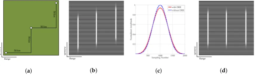
Taking the multi-channel TOPS mode as an example, a simple simulation is developed using the parameters listed in Table1. Figure5shows the results after pre-processing. Three points are located at different range and azimuth positions in the scenario in Figure5a. With DRR error (δ=0.03), signal shift occurs after pre-processing in Figure5b, whereas the time ranges{t}of three point targets are aligned after pre-processing without DRR error in Figure5d. The number of samples clearly increase for DRR error in Figure5c.

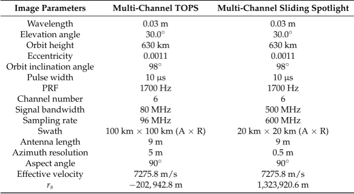
Table 1.Simulation parameters.

Image Parameters Multi-Channel TOPS Multi-Channel Sliding Spotlight

Wavelength 0.03 m 0.03 m

Elevation angle 30.0◦ 30.0◦

Orbit height 630 km 630 km

Eccentricity 0.0011 0.0011

Orbit inclination angle 98◦ 98◦

Pulse width 10µs 10µs

PRF 1700 Hz 1700 Hz

Channel number 6 6

Signal bandwidth 80 MHz 500 MHz

Sampling rate 96 MHz 600 MHz

Swath 100 km×100 km (A×R) 20 km×20 km (A×R)

Antenna length 9 m 9 m

Azimuth resolution 5 m 0.5 m

Aspect angle 90◦ 90◦

Effective velocity 7275.8 m/s 7275.8 m/s

A

zim

ut

h

Range

50km

50km

50

k

m

50

k

m

(a)

A

zim

ut

h

Range

(b) (c)

A

zim

ut

h

Range

(d)

Figure 5.Demonstration of the influence of DRR: (a) shows a scene with three target points located at different range and azimuth positions; (b) illustrates the symmetrical shift of the azimuth signal after pre-processing with DRR error; (c) shows the scaling effect of the azimuth signal after pre-processing with DRR error; (d) the result of pre-processing without DRR error.

3.2. Estimation of the DRR Error

Based on the analysis on the effects of DRR error, a novel estimation method is proposed in this section, which contributes to the imaging processing of multi-channel BS-SAR. The central positions of signals coming from different point targets in azimuth after pre-processing will overlap without DRR error, while they will shift when DRR error occurs (see (27)). Assume there are two point targets located at (r,vt1) and (r,vt2), and the time interval between them is

∆_{t= (t2−t1)}

α(r). (30)

Then the time shift between the targets after pre-processing is

∆ts1= δ

(1+δ)

(t2−t1)

α(r) . (31)

Therefore, the DRR error can be obtained as

δ= ∆ts1/∆t

1−∆_ts1/∆_t, ∆kω=

δ 1+δk

e

ω(1+δ). (32)

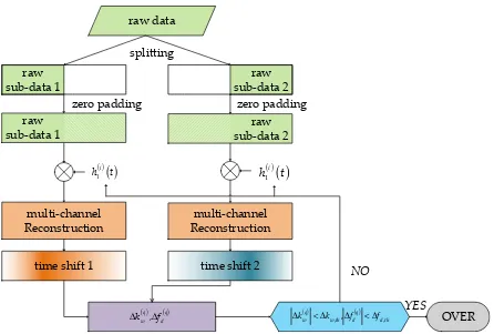
Since the raw data are a collection of echoes reflected by all scatterers on the ground, we cannot separate the echoes of two point targets from the raw data. If we split the raw data into two equal parts and extend them to the same size as the whole data by zero-padding, we obtain two images after the pre-processing. Although the envelopes of different targets in each image do not perfectly overlap due to their different locations, the whole envelope will also shift some pixels from the center of the image after pre-processing. So, the formula (32) derived for the point target echo will also apply to the raw data.

The raw data is split into two equal parts in azimuth. To hold the timing positions of sub-data, zero-padding is performed as shown in Figure6. The zero-padded sub-data are then pre-processed. The time shift between the products of pre-processing can be obtained using image registration. Finally, the DRR error can be determined by (32). Since the time shift is estimated from image amplitude, the last phase multiplication in pre-processing can be ignored.

3.3. Estimation of the CDC Error

similarly to the azimuth antenna pattern. So, the methods in [30], such as power balance and peak detecting, can be used on the pre-processed signal to estimate the CDC. In this section, these methods are extended to be used in the estimation of CDC error.

raw

sub-data 2

raw

sub-data 1

raw

sub-data 2

raw

sub-data 1

time shift 1

raw data

splitting

multi-channel

Reconstruction

multi-channel

Reconstruction

( )

( )

i

h t h₁( )i

_{( )}

time shift 2

OVER

YES

NO

( ) ( )

, , ,

q q

w w th d d th

k k f f

∆ < ∆ ∆ < ∆

( ) ( ) ,

q q

w d

k f

∆ ∆

zero padding

zero padding

Figure 6.Flowchart of the method to estimate DRR and CDC errors.

If there is a CDC error,∆_{fd, the signal after the first phase multiplication withh}(i)

1 (t)will include

∆fd. Due to the transformation of the pre-processing, the Doppler shift introduced by a CDC error can be seen as a time delay in the signal after pre-processing as

se_c(t;r,t0) =rect



 

t+ ∆fd

keω −

δ

(1+δ)α(r)t0

X_f(r)

v rs

r (1+1δ)

1−_α(δ_r)rr_s 



rect

_vt

0 Xs

exp

jπ k e ωfr ke

ω−fr( t−t0)2

. (33)

From (33), it can be seen that the time range{t}of a point target is shifted by the DRR error and CDC error. So, the CDC error can be integrated into the estimation of DRR error. The time delay of an arbitrary point target after pre-processing with DRR error and DC error is given by

ts2= δ

(1+δ)

t0 α(r)−

∆fd ke

ω

. (34)

For two point targets located at (r,vt1) and (r,vt2), the time delays after processing are

 



ts2,1 = ₍₁₊δ_δ)αt₍1_r)−

∆fd

ke ω

ts2,2 = ₍₁₊δ_δ)αt₍2_r)−

∆fd

ke ω

(35)

∆_fd=−1

2k e

ω(ts2,1+ts2,1). (36) The flowchart of the estimation of DRR error and CDC error is shown in Figure6. To obtain sufficient precision, the estimation procedure can be iterated until the termination condition is met as

∆k

(q)

w

<∆kw,th, ∆f

(q)

d

<∆fd,th, (37)

where∆_k(_wq)_and∆_f(q)

d are the estimated DRR and CDC error after theq-th iteration respectively and

∆_kw,thand∆_{fd,thdenote their thresholds for the precision.}

3.4. Estimation for Phase Inconsistency Errors

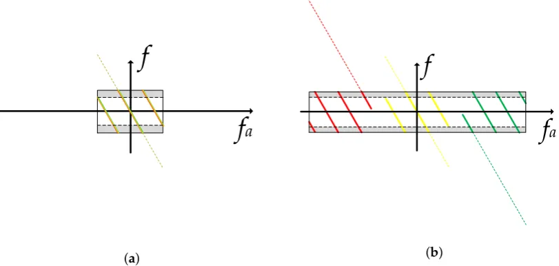
Phase inconsistency error estimation is important for fine spectrum reconstruction and imaging in multi-channel SAR systems. The existing estimation methods for multi-channel strip-map SAR are mainly based on the MUSIC method [21]. This kind of methods are all based on the frequency consistency of all signals from different azimuth positions. In multi-channel strip-map SAR, all the signals from different targets will overlapped in Doppler domain as in Figure7a. It can be seen that there are two ambiguous spectra in the grey parts, which can be used to construct the covariance matrix of Doppler spectrum. Then the signal subspace and the noise subspace can be extracted and are used to calibrate the phase inconsistency errors. However, in the multi-channel BS-SAR (Figure7b), the Doppler spectrum of targets at different azimuth position is not overlapped because of the azimuth-varying Doppler centroid. Therefore, it is impossible to determine the ambiguity number in a certain Doppler gate and there is not appropriate spectrum that MUSIC method can employ.

f

a

f

(a)

f

a

f

(b)

Figure 7. The Doppler frequency aliasing in multi-channel strip-map SAR (a) and multi-channel BS-SAR (b). The three colors represent three targets in azimuth.fandfadenote the baseband frequency and physical frequency, respectively.

Image Entropy is then adopted to assess how well the spectrum is concentrated after pre-processing. The advantage of using image entropy is that it can simultaneously evaluate the spectrum inside and outside the effective bandwidth, which can achieve better performance that AWSL and DSO. Another benefit of using the whole spectrum is that the CDC error can be ignored while the AWLS and DSO methods require knowledge of the CDC.

Usingmandlto represent the azimuth and range pixel indices respectively, rewrite Equation (12) in discrete form with phase inconsistency errors:

˜Sa(m,l) =ΓH(m)Ua(m,l), (38)

where ˜Sa(m,l)is the discrete form ofSa(f,r)with phase inconsistency errors, given as

˜Sa(m,l) =

h

˜

S(a0)(m,l), ˜S(a1)(m,l),· · ·, ˜Sa(N−1)(m,l)

iT

(39)

andΓ_{is the phase inconsistency error matrix:}

Γ_{=diag{g}=diag}nejξ0_{, e}jξ1_{,· · ·, e}jξN−1o_{. (40)}

The unambiguous spectrumUa(m,l)can then be estimated by

Ua(m,l) =P(m)Γ−1˜Sa(m,l), (41)

whereP(m)is the discrete form ofP(f)in (15). ThenUa(m+n·fpr f;l)can be re-expressed as Ua

m+n·fpr f;l

=gHdiag{Pn(m)}˜Sa(m,l). (42)

The image entropy involving phase inconsistency error is then given as

Φ=−

∑

∑

N

∑

Ua

m+n·fpr f;r

·UH a

m+n·fpr f;r

Ez ln

Ua

m+n·fpr f;r

·UH a

m+n·fpr f;r

Ez

=−

∑

∑

N

∑

gH·Ω·g

Ez ln

gH·Ω·g

Ez

, (43)

where[•]Hrepresents conjugate-transpose and

Ω_=diag{Pn(m)}˜S_a(m,l)˜S_a(m,l)H_diag

Pn(m)∗ , (44)

Ez=

∑

The optimization can be expressed as

∧

g=arg min

g

−

∑

l

∑

m N

∑

n=1 gHΩ_g

Ez ln gHΩ_g

Ez . (46)

To solve the optimization problem, the cyclic coordinate iteration is needed, in which we minimize the objective function on one channel error at a time while holding all other channels fixed. In each iteration, the optimum algorithms, such as gradient descent and Newton-like algorithm, can be used. Reference [29,35] give a fast convergence algorithm that can also be introduced here. A kind of closed-form solution in each iteration can be obtained by constructing a surrogate function, which has high convergence rate. The termination threshold for iterations is set as

whereΦ_{qis the image entropy afterq-th iteration and}∆Φ_{thdenotes the threshold for the precision.}

The small∆Φ_{th, the higher the precision and the greater the computational load.}

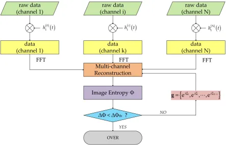
Since the estimation method is based on the minimum entropy, it can be named as minimum entropy (ME) method. The flowchart for this estimation method is given in Figure8. Because the errors usually interact with each other in practice, we perform the estimations in Figures6and8alternately to give high estimation precision. Notice that the proposed ME method in our manuscript is different from conventional minimum-entropy-based autofocusing. Because the proposed method is performed in Range-Doppler domain before the imaging processing and focuses on the phase inconsistency errors between different channels while MEBA is targeted at azimuth phase error in image domain.

data

(channel 1)

data

(channel k)

data

(channel N)

FFT

FFT

FFT

Multi-channel

Reconstruction

raw data

(channel 1)

raw data

(channel i)

raw data

(channel N)

( )0

_{( )}

h t ( )

( )

1

i

h t ( )N

( )

1

h t

Image Entropy

<

?

OVER

YES

NO

{

_e

_,e

_,

_,e

}

=

g



Figure 8.Flowchart of the method to estimate phase inconsistency errors.

3.5. Weighting for Estimation

In the previous discussion, it was seen that the shape of the pre-processed spectrum is important in estimating DRR error, CDC error, and phase inconsistency errors. In practice, however, thermal noise may affect the pre-processed spectrum. Reference [12] demonstrates that the output noise power after reconstruction can be amplified for the case of highly non-uniform sampling. The uniformity factorFu can be defined as

Fu = fpr f fpr f,uni

=N·d.v.fpr f

, (48)

wheredis the effective distance between adjacent channels. In [7], the signal-to-noise ratios (SNR) scaling factor, which quantifies the amplified degree of output noise power due to filter reconstruction, is defined as

Φ_{b f =}

SNR_in SNRout

SNRin

SNRout

_PRF

uni

= 1

σ2 1

+ 1

σ2 2

+· · ·+ 1

σ2 N

whereSNRinandSNRoutare the SNR before and after filter reconstruction, respectively, andPRFuni represents the PRF corresponding to uniform space sampling. Hereσ1,σ2,· · ·,σN are the singular values of matrixH(see (11)). For the uniform case (Fu= 1), the SNR scaling factor is 1. When the system works with non-uniform PRF, the correlation between the adjacent row vectors inHwill increase, which results in small singular values, so the SNR scaling factor will increase. More information on the SNR scaling factor can be found in [7].

An example of an amplified noise spectrum is shown in Figure9a. It can be seen the noise spectrum components at the edge of the bandwidth dominate the degradation of SNR. When the SNR is low, the noise power may exceed the signal power at the edge of the bandwidth, which will degrade the performance of the proposed estimation methods. According to [31], the normalized noise spectrum can be got by reconstruction matrix, given as

Snoise(f+k·fpr f) =kPk(f)k22. (50)

(a) (b) (c)

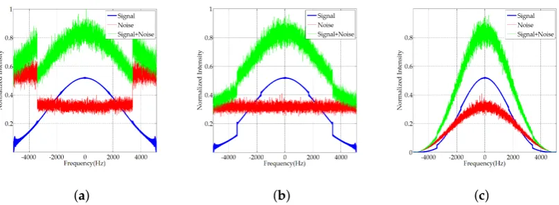
Figure 9.Weighting of spectrum for estimation. (a) shows the spectrum of signal, noise and noised signal after pre-processing without weighting; (b) is the spectrum of signal, noise and noised signal after pre-processing weighted byF1(f); (c) is the spectrum of signal, noise and noised signal after pre-processing weighted byF2(f).

Then a natural weighting function can be formulated to suppress the noise spectrum components as

F1(f) = 1

Snoise(f). (51)

Evidently, the noise spectrum can be flattened with a uniform floor by using the weighting filter in Equation (51). Since the estimation of the DRR and CDC errors is based on the maximum of the spectrum, the weighted spectrum will became more concentrated (see Figure9b) and the effect of noise will be significantly reduced. For the phase inconsistency errors, however, the noise spectrum at the edge of the bandwidth will still reduce the estimation performance and even cause the iteration to converge to the wrong value. To tackle this problem, we modify Equation (51) as

F2(f) = win(f)

Snoise(f)

, (52)

segment of the spectrum. After using the weighting function in (52), the estimation method for phase inconsistency errors will get better performance.

4. Experiments and Discussion

In this section, simulated multi-channel BS-SAR data are used to assess the performance of the proposed method to estimate the DRR error, CDC errors, and the phase inconsistency errors. For convenience, the phase inconsistency errors are called PI errors for short in Tables2and3.

Table 2.Experiments results of CDC error, DRR error, and the phase inconsistency errors.

Errors Multi-Channel TOPS Multi-Channel Sliding Spotlight True Value Estimated Value Error True Value Estimated Value Error

DRR error 530.8 Hz/s 531.15 Hz/s 0.35 Hz/s 70.6 Hz/s 70.1 Hz/s 0.5 Hz/s

CDC error 100 Hz 100.24 Hz 0.24 Hz 100 Hz 100.32 Hz 0.32 Hz

PI error (Channel 1) 0◦ 0◦ 0◦ 0◦ 0◦ 0◦

PI error (Channel 2) 30◦ 29.89◦ 0.11◦ 30◦ 29.87◦ 0.13◦

PI error (Channel 3) −24◦ −23.85◦ 0.15◦ −24◦ −24.05◦ 0.05◦

PI error (Channel 4) 24◦ 23.92◦ 0.08◦ 24◦ 23.89◦ 0.11◦

PI error (Channel 5) −10◦ −9.98◦ 0.02◦ −10◦ −9.97◦ 0.03◦

PI error (Channel 6) 5◦ 4.89◦ 0.11◦ 5◦ 5.12◦ 0.12◦

Table 3.Image quality indicators of the point targets located at the scene edge.

Multi-Channel TOPS

Azimuth Range _Normalized

Amplitude Resolution (m) PSLR (dB) ISLR (dB) Resolution (m) PSLR (dB) ISLR (dB)

No Error 3.35 −13.27 −10.06 3.33 −13.27 −10.04 1.00

DRR Error 3.46 −13.24 −10.67 3.33 −13.26 −10.04 0.98

CDC Error 4.40 −12.68 −15.07 4.24 −24.61 −23.06 0.41

PI errors 3.35 −11.26 −8.49 3.33 −13.28 −10.04 0.96

Multi-Channel Sliding Spotlight

Azimuth Range _Normalized

Amplitude Resolution (m) PSLR (dB) ISLR (dB) Resolution (m) PSLR (dB) ISLR (dB)

No Error 0.31 −13.27 −10.46 0.34 −13.20 −10.55 1.00

DRR Error 0.32 −14.07 −11.51 0.34 −13.20 −10.58 0.97

CDC Error 0.31 −13.26 −10.42 0.34 −13.23 −10.56 0.99

PI errors 0.31 −11.97 −9.00 0.34 −13.28 −10.56 0.33

4.1. Point Targets Simulation Experiments

The parameters in Table1are used in the simulation experiment. The DRR error, CDC error, and phase inconsistency errors are shown in Table2. The effects of these errors are first simulated. The SNR is set as 20 dB in this experiment. The Doppler spectrum of multi-channel TOPSAR after pre-processing with different kinds of errors are shown in Figure10while the Doppler spectrum of multi-channel sliding spotlight is similar and omitted for briefness. However, the estimation results for both modes are shown in Table2. Then the imaging results for both modes are presented in Table3.

(a) (b)

Figure 10.Azimuth signals of multi-channel TOPSAR after pre-processing: (a) shows the amplitude of signals with DRR error (dotted green line), CDC error (dashed blue line), phase inconsistency errors (dash-dot yellow line) and without error (red line); (b) shows the amplitude of the signals after antenna correction.

These impacts are more obvious after antenna correction (Figure10b). The Doppler spectrum is deformed by DRR error and becomes tilted due to CDC error. Please note that the shape of the overall spectrum with DRR error is not the same as for arbitrary targets because the spectra of point targets located at different positions with DRR error are not located in same spectral interval. Since the spectrum is reconstructed by segment (see Ua(f+k·fpr f;r) in (14)), the phase inconsistency errors will disturb the weights ofSa(k)(f,r)in each segment. Therefore, the spectrum with phase inconsistency errors becomes discontinuous and unsteady. The effects of these errors on Doppler spectrum in multi-channel sliding spotlight SAR are similar and are omitted here.

The imaging results, azimuth profiles and quality indicators of the point targets located at the scene edge are shown in Figure11and Table3. It can be seen that azimuth resolution with DRR error degrades seriously because part of the spectrum is outside the effective bandwidth. The amplitude of the target also decreases due to imperfect azimuth antenna pattern correction and spectrum loss. From Figure11f, the first null points of azimuth profile are about−25 dB, which cannot meet the quality of application in practice (−40 dB). The CDC error seriously affects the image (Figure11g) because the range cell migration is not corrected completely. In addition, both the Peak Sidelobe Ratio (PSLR) and Integrated Sidelobe Ratio (ISLR) decrease with phase inconsistency errors and the amplitude decreases as well. Overall, the effects of these errors on multi-channel sliding spotlight is smaller than multi-channel TOPS. Since the azimuth swath in multi-channel sliding spotlight is smaller, which leads the effect of DRR error smaller. CDC error also has much less impact on multi-channel sliding spotlight. However, the intensity loss is much seriously in multi-channel sliding spotlight than multi-channel TOPS.

4.2. Performance Analysis of Estimation Methods

SAR is similar with multi-channel TOPSAR, the performance is analyzed based on multi-channel TOPSAR for convenience. For the phase inconsistency errors, the root-mean-square error (RMSE) is defined as:

σ= v u u

t 1

N−1 N

∑

n=1

_∧

ζi−ζi

2

, (53)

whereζ∧iis the estimate ofζi.

(a) (b) (c) (d)

(e) (f) (g) (h)

(i) (j) (k) (l)

(m) (n) (o) (p)

The performance of the DRR error estimation method against SNR andFuis shown in Figure12. The estimation errors for DRR decrease as SNR increases for both values ofFuused, but the estimation error forFu= 0.9 is much larger than the figure forFu= 1.05. This can be explained by the azimuth ambiguity signal rate. WhenFu= 0.9, the operating PRF of the system is lower than in the uniform case. As a result, more ambiguous power is aliased into the processing bandwidth. The fluctuation atFu= 1.1 when SNR = 0 dB in Figure12b can be explained by the same. As the estimation precisions of DRR error can also be impacted by the azimuth ambiguity signal rate, expect the SNR. WhenFuincreases from 1 to 1.2, the SNR scaling factor (see (49)) will increase, which will degrade theSNRoutand result worse estimation precision. On the other hand, largerFumeans larger PRF and less ambiguity signal rate according the sampling theory. Then the less ambiguity will alleviate the negative tendency of estimation precision brought by worseFu. In the case here, the scaling factor domains the upward tendency of estimation precision fromFu= 1 toFu= 1.1 and then the ambiguity signal rate becomes the dominated factor afterFu= 1.1. It also can be seen that this conflict between scaling factor and ambiguity signal rate is depended on the SNR. When SNR is large enough (e.g., 20 dB), the estimation error has no obvious correlation with the uniformity factor.

(a) (b)

Figure 12.The performance of DRR error estimation method versusSNR(a) andFu(b).

The performance of the CDC error estimation methods against SNR andFuis shown in Figure13. In this experiment, we compare the SCCC method with the symmetric shift (SS) method proposed in this paper. The SS method achieves slightly better precision than SCCC for all SNR and is robust against the uniformity factorFu, while the SCCC method is sensitive toFu. This is because the SCCC method depends on the correlation between the adjacent pulses. As theFuincreases, the estimation error of SCCC method has the increasing tendency. The drop atFu= 1.1 is only a bad case, which should be ignored. The figures for proposed SS method at SNR = 0 dB have not obvious correlation withFu, which indicates SS method is not sensitive toFu, because SS method is based on the shift between two images after pre-processing, which will partly neutralize the error due to increasingFu. Therefore, the SS method is in most cases more accurate a bit.

Fuchanges from 1.15 to 1.2 is an artefact caused by the covariance matrix becoming singular when coincident sampling [31–33] occurs, i.e., the sampling of the first channel for one pulse coincides with the sampling of the last channel for the previous pulse, but the proposed method would not be affected in case of coincident sampling.

(a) (b)

Figure 13.The performance of CDC error estimation method versusSNR(a) andFu(b).

(a) (b)

Figure 14.The performance of CDC error estimation method versusSNR(a) andFu(b).

4.3. Distributed Targets Simulation Experiments

targets, the CDC error is another factor that leads the smeared effect. It is not easy to see the effects of DRR error in the image directly because it mainly has an effect on the azimuth resolution and intensity loss. After error correction, the image (Figure15c) is well focused, as same as the image simulated without errors (Figure15a).

A

zim

ut

h

Range

(a)

A

zim

ut

h

Range

(b)

A

zim

ut

h

Range

(c)

Figure 15.Simulated results from distributed targets: (a) is the image without errors, (b) is the image with errors and (c) is after error correction.

5. Conclusions

Multi-channel BS-SAR is a promising approach for high resolution and wide-swath observation, but is subject to errors that can lead to degradation of image quality. To overcome spectrum aliasing caused by beam steering and non-uniform sampling of the azimuth channels, pre-processing, combined with derotation and spectrum reconstruction, is used by most multi-channel BS-SAR imaging algorithms; this requires accurate system parameters and error calibration. However, the derotation rate error is not always accurately calculated, and the constant Doppler centroid and phase inconsistency errors cannot be calibrated by conventional methods. The interaction between different errors also makes the error estimation more difficult.

Phase inconsistency errors between azimuth channels are inherent in multi-channel SAR systems but most estimation methods for multi-channel strip-map SAR cannot be used in multi-channel BS-SAR because the spectra of different azimuth targets are separated in the Doppler domain, which prevents the use of traditional MUSIC methods. Methods based on the spectrum energy distribution are applicable to multi-channel BS-SAR but are sensitive to the CDC error because they depend on the spectrum only inside or outside the processing bandwidth. To overcome this, we use a minimum entropy estimation method based on the full spectrum which is robust against the CDC error. With the help of novel weighting strategy, the ME method can achieve excellent performance even in bad SNR and uniformity factor. Estimation and correction simulations demonstrate its excellent performance.

Author Contributions:H.G. and W.Y. conceived and developed the methods and performed the experiments; J.C., S.Q. and C.L. supervised the research; and H.G. wrote the paper.

Funding:This research received no external funding.

Acknowledgments:This work is supported by the National Natural Science Foundation of China (NSFC) under Grant No. 61861136008 and Grant No. 61701012, Fundamental Research Funds for the Central Universities under Grand No. YWF-19-BJ-J-304 and China Scholarship Council (CSC) under Grant No. 201806020013.

Conflicts of Interest:The authors declare no conflict of interest.

Appendix A

This appendix derives time range{t}given by (24) lies inside{t}given by (25). For clarity, we use t(1)_andt(2)_{reference time range{t}in (24) and (25), respectively. If we can prove the following}

two items:

1. The lower boundary valuet(_l1)oft(2)is larger than the lower boundary valuet(_l2)oft(2); 2. The upper boundary valuet(r1)oft(1)is less than the upper boundary valuet(r2)oft(2).

The ranges oft(1)andt(2)whent0=−Xs

2v andt0=

Xs

2v are derived as

t(1)

_t

0=−Xs/(2v) ∈

− δ

(1+δ)α(r)

Xs

2v−

1 2

X∆θ(r)

(1+δ)v

rs r − δ α(r)

,

− δ

(1+δ)α(r)

Xs

2v+

1 2

X∆θ(r)

(1+δ)v

rs r − δ α(r)

, (A1)

t(1)

_t

0=Xs/(2v) ∈

δ

(1+δ)α(r)

Xs

2v−

1 2

X∆θ(r)

(1+δ)v

rs r − δ α(r)

,

δ

(1+δ)α(r)

Xs

2v+

1 2

X∆θ(r)

(1+δ)v

rs r − δ α(r)

, (A2)

t(2) _t

0=−Xs/(2v) ∈ −r e s r Xs 2v −

1 2Tw

res r −1

,−r

e s r

Xs 2v +

1 2Tw

res r −1

, (A3)

t(2) _t

0=Xs/(2v) ∈

res r

Xs 2v −

1 2Tw

res r −1

,

res r

Xs 2v +

1 2Tw

res r −1

. (A4)

Thent1andt2can also be expressed as

t(1)= t(1) _t

0=−Xs/(2v)

+ δ

(1+δ)α(r)

Xs 2v +t0

, (A5)

t(1)= t(1) _t

0=Xs/(2v)

− δ

(1+δ)α(r)

Xs 2v −t0

, (A6)

t(2)= t(2) _t

0=−Xs/(2v) +r e s r _X s 2v +t0

, (A7)

t(2)= t(2) _t

0=Xs/(2v) −r e s r Xs 2v −t0

. (A8)

t_l(1)−t_l(2)= t(_l1) _t

0=Xs/(2v)

− δ

(1+δ)α(r)

Xs 2v −t0

−t(_l2)

_t

0=Xs/(2v) +r e s r Xs 2v −t0

= ∆tl(t0)|t0=Xs/(2v)+

re_s r −

δ

(1+δ)α(r)

Xs 2v −t0

, (A9)

where

∆_tl(t0)|t

0=Xs/(2v)= t

(1)

l

_t

0=Xs/(2v) −t(_l2)

_t

0=Xs/(2v)

= δ

(1+δ)α(r)

Xs 2v −

1 2

X∆θ(r)

(1+δ)v

_r

s r −

δ α(r)

−r e s r Xs 2v+

1 2Tw

_re s r −1

= δ

(1+δ)α(r)

Xs+X∆θ(r)

2v −

res r

Xs+X∆θ(r)

2v +

1 2Tw

res r −1

= δ

(1+δ)

Tw 2 −

re s r

Twα(r)

2 +

1 2Tw

_re s r −1

= δ

(1+δ)

Tw

2 + (1−α(r)) re_s

r Tw

2 − 1 2Tw

= δ

(1+δ)

Tw 2 +

res r

Tw 2 −

1 2Tw=

δ

(1+δ)

Tw 2 +

1

(1+δ)

Tw 2 −

1 2Tw=0

. (A10)

Notice that we have used (22) and the following equation

X∆θ(r) +Xs =vTwα(r). (A11)

Therefore,

t(_l1)−t(_l2)=

res r −

δ

(1+δ)α(r)

Xs 2v −t0

= 1

α(r)

α(r)r

e s r −

δ

(1+δ)

Xs 2v −t0

= 1

α(r)

rs−r rs

re_s r −1+

re_s r

Xs 2v −t0

= 1

α(r)

re_s r −1

Xs 2v −t0

>0

. (A12)

Next, substitute (A5) and (A7) into∆_tr(t0)as

tr(1)−tr(2)= t(r1)

_t

0=−Xs/(2v)

+ δ

(1+δ)α(r)

Xs 2v +t0

−t(r2)

_t

0=−Xs/(2v) −r e s r Xs 2v +t0

= ∆tr(t0)|t0=−Xs/(2v)+

_δ

(1+δ)α(r) −

re s r

Xs 2v +t0

, (A13)

where

∆_tr(t0)|t

0=−Xs/(2v)= t

(1)

r

t0=−Xs/(2v) −t(r2)

t0=−Xs/(2v)

=− δ

(1+δ)α(r)

Xs 2v +

1 2

X∆θ(r)

(1+δ)v

rs

r −

δ

α(r)

+res

r Xs 2v −

1 2Tw

re

s

r −1

=0

(A14)

as similar to (A10). Therefore,

t(r1)−t(r2)=

δ

(1+δ)α(r)−

res r

Xs 2v +t0

= 1

α(r)

1−r

e s r

Xs 2v +t0