Use of near-infrared photogrammetry to determine crack and surface deformation in small structures

University of Southern Queensland

Faculty of Engineering and Surveying

Use of Near-infrared Photogrammetry to

Determine Crack and Surface

Deformation in Small Structures

A dissertation submitted by

Paul David Lenton

In fulfilment of the requirements of

Courses ENG4111 and 4112 Research Project

Towards the degree of

Bachelor of Spatial Science (Survey)

Abstract

The purpose of this Research Project was to compare conventional (colour) photogrammetry with near-infrared photogrammetry to determine whether the use of near-infrared photogrammetry is a suitable method for measuring structural deformation. To undertake this, laboratory testing was conducted by Mr. Daniel Pratt (as part of his undergraduate thesis) under controlled circumstances on a number of structural materials to gauge whether there was a significant difference between the two methods of photogrammetry. Anecdotal evidence provided by Mr. Pratt suggested there were no significant differences in method and that near-infrared photogrammetry was a suitable method.

This Research Project then examined the two photogrammetric methods on the Hodgson Creek bridge, located at Eton Vale, approximately 16km southwest of Toowoomba on the New England Highway. Both diffuse and retro-reflective targets were used for this project, with the targets placed upon Pier 4 of this structure. A control traverse, using conventional total station equipment was used to place control station under the structure and locate targets on the pier headstock to within ±0.002m. Image capture was conducted at night with the resulting stereo images imported into the Australis v6.0 photogrammetric software package for processing.

Disclaimer

University of Southern Queensland

Faculty of Engineering and Surveying

ENG4111 and 4112 Research Project

Limitations of Use

The Council of the University of Southern Queensland, its Faculty of Engineering and Surveying, and the staff of the University of Southern Queensland, do not accept any responsibility for the truth, accuracy or completeness of material contained within or associated with this dissertation.

Persons using all or any part of this material do so at their own risk, and not the risk of the Council of the University of Southern Queensland, its Faculty of Engineering and Surveying or the staff of the University of Southern Queensland.

This dissertation reports an educational exercise and has no purpose or validity beyond this exercise. The sole purpose of the course pair entitled “Research Project” is to contribute to the overall education within the student’s chosen degree program. This document, the associated hardware, software, drawings, and other material set out in the associated appendices should not be used for any other purpose: if they are so used, it is entirely at the risk of the user.

Prof Frank Bullen

Dean

Candidates certification

Certification

I certify that the ideas, designs and experimental work, results, analyses and conclusions set out in this dissertation are entirely my own effort, except where otherwise indicated and acknowledged.

I further certify that the work is original and has not been previously submitted for assessment in any other course or institution, except where specifically stated.

Paul David Lenton

Student Number: 0050078460

Signature

Acknowledgements

First, I would like to acknowledge my project supervisor, Dr. Albert Chong for his help and guidance throughout this year. His knowledge and willingness to provide assistance when required has proved to be invaluable.

I would also like to thank my friend and manager, Mr. Eric Brown of the Department of Transport and Main Roads for the use of Departmental equipment and vehicles to undertake the fieldwork component of this project, as well as any time off to undertake these studies, when required.

Table of contents

Abstract i

Disclaimer ii

Candidates certification iii

Acknowledgements iv

Table of contents v

List of figures vii

List of tables viii

List of appendices 8

1 Introduction 9

1.1 Outline of the study 9

1.2 Introduction 9

1.3 Reason for study 11

1.4 Research aim and objectives 12

1.4.1 Aim 12

1.4.2 Objectives 12

2 Literature review 14

2.1 Introduction 14

2.2 The electromagnetic spectrum 14

2.2.1 Concept of electromagnetic wavelengths 14

2.2.2 The visible light spectrum 16

2.2.3 The infrared spectrum 17

2.3 Structural deformation 18

2.3.1 What is structural deformation? 18

2.3.2 Current methods for measuring structural deformation 19

2.4 Photogrammetry 20

2.4.1 What is photogrammetry? 20

2.4.2 Brief history on photogrammetry 22

2.4.3 Advantages and disadvantages of photogrammetry 23 2.5 Important mathematical concepts behind photogrammetry 24

2.5.1 Determining three-dimensional measurements from

photographs 25

2.6.1 Camera calibration 28

2.6.2 Camera geometry and network 31

2.6.3 Camera sensors 35

3 Research design and methodology 37

3.1 Laboratory testing 37

3.1.1 Materials and equipment 37

3.1.2 Control points and camera calibration 38 3.1.3 Image capture and processing of acquired images 39

3.2 Field testing 39

3.2.1 Structure selection 39

3.2.2 Establishment of control 40

3.2.3 Image capture and processing of acquired images 44

4 Results 48

4.1 Background relating to the results 48

4.2 Issues associated with the reporting of results 49

4.3 Target acquisition 49

4.3.1 Diffuse targets 49

4.3.2 Retro-reflective targets 51

4.3.3 Distance comparisons 53

5 Analysis and Discussion 55

5.1 Commentary on results 55

5.2 Potential benefits between photogrammetric methods, and over

traditional survey methods 56

5.3 Problems and issues encountered during the field testing and

processing activities 58

5.4 Recommendations and further research 66

6 Conclusions 68

List of figures

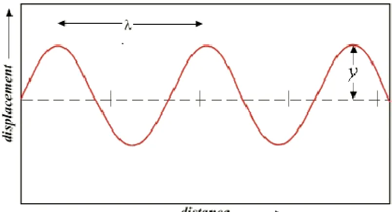
Figure 1. A typical sinusoidal wave, showing the wavelength (λ) and

amplitude (γ) of a given wave. 15

Figure 2. A typical electromagnetic wave, showing the vertical displacement of the electric wave (in red) and the horizontal displacement of the magnetic field (in blue). 15

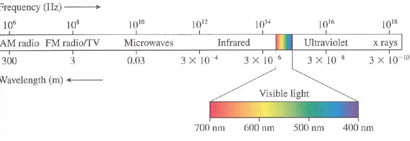
Figure 3. The electromagnetic spectrum. 16

Figure 4. Projection of the single ray to determine direction in space. 25

Figure 5. Using the intersection of two single rays to determine object

position. 26

Figure 6. Using multiple rays to determine the position of a number of

objects within a single image. 26

Figure 7. Minimising the area of uncertainty 32

Figure 8. Principal photogrammetric network configurations. 32

Figure 9. Stereoscopic image configurations. 34

Figure 10. The Hodgson Ck bridge at Eton Vale. 40

Figure 11. An example of the target placement and location on the

Hodgson Creek bridge pier headstock. 42

Figure 12. Target acquisition under bright light conditions. 44

Figure 13. Target acquisition under total darkness utilising the infrared

emitter attached to the camera. 45

Figure 14. The effect of blooming on retro-reflective targets. 59

Figure 15. Differences in near-infrared emitter. 61

Figure 16. Example of the narrow field of view of the emitted

List of tables

Table 1. Main parameters used in the 12d data reduction process. 41

Table 2. Camera parameters used in the Australis software processing. 45

Table 3. Camera parameters used in the Australis software processing

for the additional photographs. 46

Table 4. Test-point comparison between the control and diffuse colour

targets. 50

Table 5. Test-point comparison between the control and retro-reflective

colour targets. 51

Table 6. Test-point comparison between the control and near-infrared

retro-reflective targets. 52

Table 7. Comparison between the reflective colour and

retro-reflective near-infrared targets. 53

Table 8. Comparison of reduced distances between selected target

points for all image types 54

List of appendices

Appendix A: Project specifications 74

Appendix B: Control traverse report file 76

Appendix C: Target location report file 80

1

Introduction

1.1

Outline of the study

Structural deformation measurement and monitoring is of importance to those wishing to construct or utilise constructed objects, as structural failure has the potential to lead to death or serious injury to persons and/or property should a failure occur. To avoid such a consequence, photogrammetry is but one method of measurement used to determine whether deformation is, or has occurred, and the extent to which it is likely to affect the built structure.

Conventional photogrammetry uses colour photographs to determine deformation measurements. It has proven to be an effective method of determining structural deformation. However, recent evidence in other fields of study suggest that near-infrared photogrammetry may be a more accurate and precise method of determining structural deformation in small scale structures. The aim of this research project is to determine whether the hypothesis that “near-infrared photogrammetry is a suitable method for determining structural deformation”

holds true.

1.2

Introduction

Small structures, such as bridge members, are subjected to both static and dynamic stresses from the moment they are constructed. Static stresses in this instance would include the weight of the structure itself, as well as the weight placed upon the structure from adjoining members. Dynamic stresses would include the placement of the structure into position (and any harmonic or other vibrations generated in the placement of the member into position), and in the case of bridges, traffic flows across the completed structure.

not be readily seen by the naked eye. In the past, structures thought to be undergoing deformation were monitored through the use of conventional survey instruments (theodolites and steel bands, total stations, accelerometers, etc.), but the accuracy and precision of such monitoring may be questionable due to the extent and location of the deformation, errors in station setup, and so on. However in recent years, photogrammetry has been able to more accurately determine the presence, extent and measurement repeatability of any deformation process.

In essence, conventional photogrammetry as indicated above uses one or more (calibrated) cameras to obtain a series of images over a given time period to gauge the extent of the deformation process. This process utilises the visible wavelengths of the electromagnetic spectrum (0.4-0.7µm) in the same way that a person would use a camera to take an ordinary photograph. The image is then imported into a suitable software package and then examined for the presence of any deformation features. Because conventional photogrammetry uses the visible potion of the electromagnetic spectrum, a suitable light source is required for image exposure; solar radiation provides such a suitable light source, as does external light sources such as a flash or electric-powered light.

The reliance on a particular light source is a major drawback to conventional photogrammetry in that the capture of images must be undertaken in daylight, or at night/low-light periods when the object of interest is illuminated by artificial light sources. This in itself can pose safety issues, particularly where there is a risk of drivers becoming distracted or blinded by flashes or extremely bright light sources. This potentially serious safety issue is thought to be overcome using near-infrared photogrammetric techniques.

An added benefit that has evolved from using the infrared portion of the electromagnetic spectrum is the increased detail available for examination within an image. Infrared film can be used to distinguish objects of similar colours but different wavelength emission characteristics. Since World War II when photogrammetrists used infrared film to distinguish between camouflaged objects and vegetation, the infrared wavelength has been used to characterise different vegetation types, map differing geological and morphological characteristics of the earth, differentiate between varying land use patterns, and more recently, utilised in various biomedical applications. It is hypothesised that, due to the nature of the infrared portion of the electromagnetic spectrum, deformation progression within small structures may be more accurately defined and the extent of deformation characterised with greater precision, when compared to conventional photogrammetry techniques.

1.3

Reason for study

Conventional photogrammetry is a well research and respected method of measuring or monitoring deformation in built structures. Traditionally, this method uses natural or external light sources to illuminate the structure and associated target systems sufficiently so as to measure the deformation that is, or may be, occurring in the structure. However, should measurement activities take place at night, then external lighting systems have the potential to cause light nuisance to a variety of stakeholders.

Many structures that undergo photogrammetric measurement are bridge structures on local or main road systems. Not only do the external light sources impinge on the aesthetic quality of nearby residences, but of more importance is the impact that these lighting systems may have of the drivers that are utilising the structure during the measurement period. Drivers have the ability to become blinded or disorientated by the light systems, with an increase in the risk or potential of an accident occurring as a result of driver distraction.

risk of an accident occurring at a bridge site, as more often than not, the photogrammetrist will be out of sight and not requiring illumination during the period of the study. However, there is little data on the use of near-infrared photogrammetry for structural deformation measurements; near-infrared photogrammetric studies have been mostly restricted to medical applications, as outlined in studies by Chong & Matheau (2006), for example. It is hoped that this study will expand the knowledge based of near-infrared photogrammetric applications.

1.4

Research aim and objectives

1.4.1 Aim

The aim of this research project is to determine whether near-infrared photogrammetry is a suitable method to determine structural deformation in small structures. This aim will be achieved by conducting a number of laboratory and field-based testing on typical construction materials and a ‘live’ structure to test the hypothesis that near-infrared photogrammetry is suitable to undertake structural deformation monitoring.

1.4.2 Objectives

There are a number of specific objectives that will be examined to determine whether near-infrared photogrammetry is a suitable method of measuring structural deformation, and include:

• Examination of existing literature: the literature review will review a number of studies in which structural deformation has been captured by a variety of survey methods (including photogrammetry), and those results compared against each of the different survey methods. From this review, the suitability of photogrammetry as a method of structural deformation monitoring will be determined.

photography) and near-infrared photogrammetric techniques. These tests will be conducted under dark, low light and normal lighting conditions

• Assessment of photogrammetric images: to adequately assess the ability of near infrared photogrammetry to identify and measure accurately any significant differences between the two photogrammetric methods under certain pressure applications to measure beam deformation (target movement and direction, crack length, width, number, and so on, should they occur). Because of the size of this research project, the laboratory research will be conducted by Mr. Daniel Pratt and presented as part of his Research Project. A brief discussion will occur on his results to determine the relevance of his results to this Research Project..

2

Literature review

2.1

Introduction

This chapter will review some of the relevant literature associated with this project. It has been designed such that the reader will gain an understanding on the electromagnetic spectrum and the influence that it has on photogrammetry. It will also outline structural deformation and the some of the current methods that are used in measuring structural deformation. Finally, it will explain what is, and some important concepts behind photogrammetry, including a section on the mathematics used in photogrammetric processing.

2.2

The electromagnetic spectrum

2.2.1 Concept of electromagnetic wavelengths

Figure 1. A typical sinusoidal wave, showing the wavelength (λ) and amplitude (γ) of a given wave.

(source: Wikibooks, 2011).

Electromagnetic waves (refer to Figure 2), although having the characteristics of the typical sinusoidal wave are in fact waves of fields, and not of matter; Giancoli (2005) states that it is because of this property that electromagnetic waves can propagate in space. Further, Giancoli (2005) suggests that both these wave fields at any point are perpendicular to each other, and to the direction of wave travel. These wave fields consist of a mass of photons, travelling at the same velocity. A characteristic of these fields are that while the photons may have the same electromagnetic composition, yet can have a wide variance in frequency.

Electromagnetic waves are not treated in isolation as can be inferred from the above ‘simple’ diagrams, but form part of the electromagnetic spectrum. This spectrum contains radiation that range from gamma rays at one end of the spectrum, through to radio waves at the other. The electromagnetic spectrum can be seen diagrammatically in Figure 3; Knight (2004) reports these wavelengths of the spectrum have the most influence over today’s technologies, ranging in wavelength from 3x10-10nm (gamma rays) to 3x104m (radio waves). Lillesand, et al. (2004) point out that it should also be remembered that there is no clear cut dividing line between the differing portions of the electromagnetic spectrum, yet suggest some overlap may occur dependent on the remote sensing methods used to divide the various portion of the spectrum.

Figure 3. The electromagnetic spectrum. (source: Knight, 2004).

From Figure 3, it can be seen that the section entitled visible light has been highlighted. Immediately to the left of the visible light range (longer wavelength, lower frequency) is the near-infrared portion of the electromagnetic spectrum. It is these two portions of the spectrum that are of the most importance within close-range photogrammetric studies.

2.2.2 The visible light spectrum

Schlessinger (1995) states that the apparent colour(s) of an object is due to the energy reflected by that object, and the physiological and psychological response of the brain once that reflected energy strikes the retina. Making the assumption that all the wavelengths of the visible light portion of the electromagnetic spectrum could be viewed at the same time, white light is all that would be viewed. However, through the process of dispersion, the different wavelengths can be separated from each other for us to interpret as different colours. The best and most obvious form that the process of dispersion can be explained as the passing of white light through a prism; white light is split into the different wavelengths to view the myriad of colours that these wavelengths are comprised of. Alternatively, light passing through rain, forming a rainbow, achieves the same outcome as that of the prism – separation of wavelengths by apparent colour.

If the ambient light is low or non-existent, such as in a dark room, the apparent ‘blackness’ would indicate that there are no wavelengths of the visible light spectrum reaching the eye. The only way that objects could be viewed in this situation is through the use of an artificial light source such as a torch or lamp, or through a device that operates at wavelengths beyond that of visible light and into the infrared.

2.2.3 The infrared spectrum

The infrared portion of the electromagnetic spectrum occurs above that of the visible light spectrum, and in a similar way, is broken into three sub-portions – 700-1300nm (near infrared), 1300nm-3000nm (mid infrared) and 3000nm – 1mm (far infrared). Yet, unlike that of the visible light spectrum, objects viewed in the infrared portion of the electromagnetic spectrum are identified by the energy they emit rather than reflect (Schlessinger, 1995).

becoming more important on a global scale with increasing levels of airborne pollution, and allows for a cleaner, crisper picture to be produced. However, infrared spectrum imaging produces the false colour images (due to characteristics of the photographed objects’ emissions) that give a slightly different perspective on an object than humans would normally be used to identifying with that object.

Ruscelllo (2010) suggests that in the absence of special infrared film (of standard manual cameras), digital cameras capture infrared photographs through the use of an appropriate filter located at the front of the lens which blocks the visible wavelengths. Alternatively, a digital sensor can be placed in front of a special filter (infrared cut-off filter) internal to the camera. While either method is effective, these two methods used in combination ensure complete blockage of visible radiation from a captured image.

2.3

Structural deformation

2.3.1 What is structural deformation?

Structural deformation can be described as changes that occur in a structure from normal wear and tear over time, or from rapid changes that occur due to external factors applied to the structure. Indeed, Maas and Hampel (2006) loosely define structural deformation as a change in the 3-dimensional shape of an object; this assumes that there is a pre-existing knowledge of the original shape prior to change.

However, in some cases the pre-existing knowledge may not be available. Suspicion as to a deformation events’ occurrence may be present due to the appearance of small cracks or perhaps a slight bulging in the structure. In this case, the commencement of monitoring should occur as soon as practical, to provide a baseline of the integrity of the structure, such that any further monitoring will indicate the presence (or otherwise) of a deformation event.

fracture mechanics was occurring, although it was not until the 1950’s that this field of study was started to be taken seriously. The field of fracture mechanics therefore could define structural deformation as the appearance of (or the continuing of existing) cracking in a structure where the fracture magnitude, defined by the width and linear extension, significantly increases (Barazzetti & Scaioni, 2009).

2.3.2 Current methods for measuring structural deformation

Photogrammetry is but one method that is used to undertake structural monitoring tasks. However, as stated previously, most photogrammetric applications to date have used conventional (colour) photogrammetry, with little work or data currently available on infrared photogrammetric applications outside of medical applications.

Barazzetti and Scaioni (2009) and Mass and Hampel (2006) state that current methods of measuring displacement and deformation in structures is primarily through the use of wire strain gauges and inductive displacement transducers. It is recognised that these methods tend to produce one-dimensional data; to produce two- or three-dimensional data, considerable instrumental effort is required. Because of the complexity of multi-dimensional data collection, these gauges and transducers are generally ineffective in providing sufficient and conclusive data to determine structural deformation. Further, Whiteman, et al. (2002) state that they can be heavily influenced by external electromagnetic fields, and degraded results can occur once the gauges operate outside of their (narrow) linear range.

Barazzetti and Scaioni (2009) and Maas and Hampel (2006) suggest that conventional geodetic techniques involve the use of a combination of total station and inductive transducer techniques to measure (static) deformation in small structures, such as bridges. However, because of the accuracy of the total station, and the relatively small deflections expected in short span structures, such slight deformation will not be identified through conventional instrument acquisition.

is not widely used for structural deformation measurements. However, total station control measurements must be put in place for the laser scanner to be effective in measuring such fine measurements. Much of the accuracy of the laser scanner is reliant on the fact that a large point cloud is produced. It is also recognised that laser scanning cannot yet be used in isolation, but is more effective as a complementary method of deformation surveying.

Mills & Barber (2004) suggest that tape measurements and hand recording are still commonplace, though reflectorless EDM and time of flight laser scanning systems is also becoming more prevalent. Laser systems are still at a relative disadvantage with current technologies, as over lager distances the laser angle becomes more acute, therefore less precise. Further, lasers may give a false impression of the wall, particularly where the surface is disjointed or uneven, such as a brick wall. Multipath issues are a problem with laser scanners, as they rely on a clear path in order to obtain the best accuracies. At the current development stage, Mills & Barber (2004) recommend that laser scanning can be used as a complementary method.

While little work has been conducted in this area, Roberts, et al. (2010) suggests that survey-grade global positioning system (GPS) receivers may be used to undertake deformation monitoring. Studies conducted by Roberts et al., (2010) report that sub-centimetre deflections and deformations (in bridges) can be achieved with GPS; however it recognised that these studies were conducted on bridges with large span lengths, and given the (current) vertical accuracies able to be achieved with GPS, this method may not yet be suitable for the fine and precise measurements required on many structures.

2.4

Photogrammetry

2.4.1 What is photogrammetry?

and shape of objects as a consequence of analysing images that have been recorded on film or some other form of electronic media.

There are many who have attempted to define the term ‘photogrammetry’. For instance, Mikhail, et al. (2001) suggests that photogrammetry is a process of deriving metric information about an object through measurements made on photographs of that object. Mitchell (2007) continues on this definition to state that from these photographs accurate sets of coordinates can be obtained for an unlimited number of points on an object.

Broadly speaking, Jiang, et al. (2008) defines photogrammetry as a technique for determining the three-dimensional geometry of an object by analysing a series of two-dimensional photographs. These photographs are taken from at least two different camera positions (Jáuregui, et al., 2003) such that the line of sight from each point of concern on an object runs through the perspective centre of the camera.

Photogrammetry can be broken into two distinct fields – aerial and terrestrial photogrammetry. Aerial photogrammetry, as the name implies, requires photographs to be captured by means whereby the camera is not in contact with the surface of the Earth. The principle methods of aerial photograph capture is by airborne or satellite systems. Terrestrial photogrammetry then implies that the camera has some form of contact with the ground, whether hand held, tripod or even some sort of elevated platform. Terrestrial photogrammetry can be further broken down into two distinct areas – (general) terrestrial photogrammetry and close-range photogrammetry, where the distance from camera to object, and object size is less than 100m (Jiang, et al., (2008). Jáuregui, et al. (2003) suggests that the distance of close-range photogrammetry has limits of between 100mm to 100m; presumably because the closer distance cannot provide sufficient control points to produce accurate three-dimension coordinates.

2.4.2 Brief history on photogrammetry

Much of the content of this section is covered in greater detail by Mikhail et al.

(2001), Luhmann, et al. (2006) Jiang, et al. (2008).

The theory behind photogrammetry can be traced back to the late 1400’s where painters, such as a Vinci, undertook geometric studies of (and subsequently painted) objects to imply three-dimension images (Mikhail et al., 2001). Further developments continued; though cameras were not available until a number of centuries later (becoming widely used in the 1800’s), the mathematical principles behind photogrammetry were developed in other fields of study in the 1600’s and 1700’s.

In the mid-1800’s the Frenchman, Nadir, captured photographs of the countryside from balloons, and cityscapes were taken from rooftops for the purposes of constructing citywide maps. This last point was expanded on by the person who went on to become regarded as the father of photogrammetry, Laussedat, who, in 1895 developed the first suitable camera and procedure for making accurate photographic measurements (Mikhail et al., 2001; Luhmann, et al., 2006; Jiang, et al., 2008). At a similar time to Laussedat, a Prussian named Meydenbauer began recording historical monuments and buildings in photographs, later establishing a State Institute to record and house these images (Jiang, et al., 2008).

A major development in photogrammetry occurred in 1910, with the formation of the International Society of Photogrammetrists. One of the technical commissions of this society was established in 1926 which examined the specific areas of aerial, terrestrial and engineering photogrammetry (Jiang, et al., 2008), though this field of endeavour was largely ignored until the development of cheaper and faster processing systems, and affordable and accurate off-the-shelf non-metric cameras in the 1960’s and 1970’s.

Other such as Gruen (in Jiang, et al., 2008) suggest that there are four clear developmental stages of photogrammetry, being:

Era2: The period between 1984 to 1988, where the development of prototype systems, calibration mechanisms and the expansion of charged coupled devices (CCD’s), used primarily in digital camera systems significantly reduced the time and cost of photogrammetric processes;

Era 3: Expanded on the development of Era 2, the period between 1988 to 1992 saw increased research and development in the field of close-range photogrammetry and expanded on the potential uses of photogrammetry in the measurement of complex three-dimensional objects from easily acquired two-dimensional images; and

Era 4: the period since 1994 has seen the cost of high quality, non-metric cameras significantly decrease, automation processes in the off-the-shelf programs increase, and has seen the increased used of photogrammetry in the engineering field of study.

2.4.3 Advantages and disadvantages of photogrammetry

Photogrammetry is a method of surveying structural deformation that is gaining acceptance from a variety of professionals interested in measuring and monitoring deformation in built structures. Jiang, et al. (2008) and Whiteman et al., (2002) state that the main advantages include photogrammetry being a non-contact method of data acquisition that can be used to gather data in difficult-to-access areas, it is not as labour-intensive as other methods of survey commonly used in deformation measurement, it has the ability to record a large amount of data during a short period of time, and store acquired data easily in both hardcopy and electronic forms, and it is a convenient method to undertake routine monitoring tasks.

good geometric stability and provide simple interfacing at low cost. Photogrammetry also is moving toward the use of inexpensive, off the shelf cameras that are freely available to the novice user (Jiang, et al., 2008).

Because of the size of the camera unit, there are generally no restrictions regarding visibility as can be expected with GPS or even conventional survey instruments in confined spaces or in areas of cover. Jiang, et al. (2008) state that examination of results obtained in comparative tests conducted between photogrammetric systems and strain gauges, photogrammetric methods are as capable as strain and induction transducer gauges in measuring fine structural deformations with expected accuracies of between 0.1-0.2mm. In other comparative testing between convention instruments and photogrammetry, Jiang,

et al. (2008) suggests that photogrammetric methods were more efficient, easier and cost-effective than instrumental methods.

There appears to be little disadvantage in using photogrammetry to undertake deformation monitoring. Comparative tests between photogrammetry and other conventional and emergent survey techniques (i.e. laser scanners) suggest that similar (or better) results are obtained. However, in the case where any structural deformation has produce fine cracking, photogrammetry can state that separation of targets has occurred, but is unable to exactly pinpoint where the crack is until it has become visually obvious (Maas and Hampel, 2009).

2.5

Important mathematical concepts behind photogrammetry

2.5.1 Determining three-dimensional measurements from photographs

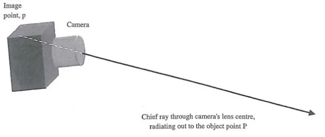
In order to acquire three dimension properties of an object of concern, it is necessary to understand an important concept, that of the principle of triangulation. Mitchell (2007) suggests that in terms of photogrammetry, it best understood by imaging a camera with a single ray projecting out of the lens of the camera toward a point on the object of concern (refer to Figure 4). This ray will have an unknown distance between the lens of the camera, but will be fixed for position and orientation by the camera.

Figure 4. Projection of the single ray to determine direction in space. (source: Mitchell, 2007)

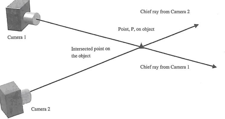
Figure 5. Using the intersection of two single rays to determine object position. (source: Mitchell, 2007)

Figure 6. Using multiple rays to determine the position of a number of objects within a single image.

(source: Mitchell, 2007)

concern, but much peripheral information that surrounds the object. Expanding on the two single ray concept above, if multiple points on the object are captured in a number of images from a number of independent stations (refer to Figure 6), then a true three dimension image of the object can be attained.

The above discussion is very simplistic. The actual coordinates will be determined in freeware or commercial photogrammetric software packages, such as Australis once the images are imported and processed through bundle adjustment. Three dimensional measurements (and the associated accuracies of those points captured within a series of images) will also be heavily influenced by the method of photogrammetric capture – single, stereo or multistation convergent methods.

2.5.2 Concept of coordinates

Mitchell (2007) suggests that the mathematical modelling behind photogrammetry adopts a number of different sets of coordinates. These are arguably the most important part of photogrammetry, as the aim of photogrammetry is to measure the difference between a set of coordinates, or to measure those differences following deformation to determine the displacement that has occurred. To this end, it is necessary to define the types of coordinates used in photogrammetry; Mitchell (2007) suggests the following definitions

• image coordinate system: the image itself has a set of coordinates based on the Cartesian coordinate systems with its origin at the centre of the image. These coordinates are generally denoted in lowercase italic x, y, z.

• object coordinate system: the structure has a set of coordinates which are often referred to as a ground coordinate system, and is also a three dimensional Cartesian coordinate system. For permanent structures, this object coordinate system is based on a State or National geodetic network, but in the case of mobile objects, takes on an arbitrary coordinates. It is usually denoted by the uppercase letters X, Y, Z.

image coordinates to produce the measurements obtained by photogrammetry.

However, because the object and image coordinates will often not be in parallel with each other, the cameras image coordinate system must be rotated to be parallel with the object coordinate system. Assuming rotation will occur (within the software package), then Mitchell (2007) states that the chief ray projecting from an image point p with image coordinates of xp, yp will travel through the lens

with object coordinates of Xi, Yi, Zi, to intersect point P on the object of concern

with coordinates Xp, YP, ZP giving rise to the collinearity equations that represent

the chief ray:

(

)

(

)

(

)

(

)

(

)

(

)

i i P i i P i i P i i p Z Z r Y Y r X X r Z Z r Y Y r X X r c x − + − + − − + − + − = 33 32 31 13 12 11

(

)

(

)

(

)

(

)

(

)

(

)

i i P i i P i i P i i p Z Z r Y Y r X X r Z Z r Y Y r X X r c y − + − + − − + − + − = 33 32 31 23 22 21 where:

r = the elements of the 3x3 rotation matrix (Mikhail, et al. (2001), utilising the three angles of rotation between the object and image coordinate system, and ci = the principal distance of the camera, determined from the camera calibration.

Mikhail et al. (2001) report that the above collinearity equations form the basis of the bundle adjustment used in photogrammetric software. However, Mikhail et al. (2001) suggests that a direct linear transformation, based on the collinearity equations, may be a more efficient process to calculate the physical position of the camera, hence the coordinates of the object of concern.

2.6

Camera properties and image acquisition

2.6.1 Camera calibration

are now adopting the use of readily available off-the shelf-cameras to undertake photogrammetric work. A primary driver behind the shift to off-the shelf-cameras in photogrammetry has been the large costs and inflexibility associated with metric cameras. However Fraser & Al-Ajlouni (2006) state that one on the largest impediments to utilising off-the-shelf digital cameras for photogrammetric purposes is the requirement to acquire images with fixed zoom and focal settings.

Determination of lens distortion parameters is critical for measurement quality. Thomas & Cantré (2009) state that many off-the-shelf digital cameras have a short distance between the lens and the sensor which achieves a large depth of field. This is advantageous because the distance between measuring points and perspective centre has no significant influence on measurement accuracy. However, digital cameras can change their optical properties easily, and often without the conscience knowledge of the user. Because of this, Jiang & Jáuregui (2010) report that the principal reason of calibration is to determine and fix the focal length, principal point and lens distortion parameters of the camera, thereby removing or minimising any systemic errors from the photogrammetric process. Mikhail et al (2001) also adds that the calibration will also determine the rotation and translation between the object space and the camera coordinate systems. Further, Thomas & Cantré (2009) suggest that every camera (metric or non-metric) not only needs to be calibrated prior to a photogrammetric exercise, but also needs to be recalibrated after each change to optical system.

Jiang & Jáuregui (2010) report that there are two main methods for camera calibration – a stand alone calibration method that utilises some form of known control, such as an Anhui dissection control plate, with or without additional scale bars, or self-calibration methods, where sufficient good quality targets acquired in a series of images from actual measurements form the basis of the calibration process. Jiang & Jáuregui (2010) suggest that self calibrating methods often yield greater accuracy as environmental variables are applied to both the calibration and the actual measurements. Additionally, the self-calibration technique does not require a set of known object-space coordinates of photographed targets (Chong & Matheau, 2006) and as such, self-calibration methods are becoming the norm for digital camera calibrations in multi-image, close-range photogrammetry (Fraser & Al-Ajlouni, 2006). While it is recognised that self calibration saves time and simplifies measurement, Woodhouse et al., (1999) warn that self-calibration techniques should be avoided where single camera stations are used, as they achieve unreliable calibration results. Interestingly Mitchell (2007) suggests another reason for calibration – correct calibration can compensate for lower optical and sensor properties of off-the-shelf digital cameras, which allow them to be used to acquire precise and accurate measurements, expected from photogrammetric studies

For the self-calibration method of camera calibrations, the images are acquired and passed into a photogrammetric software package (such as Australis) for digitising and further processing. From this, a bundle adjustment report is obtained that outlines resultant values for the interior orientation parameters of the camera, such as the principal distance, principal point offset and a number of additional parameters that correct various lens distortion qualities. Whiteman, et al. (2002) provides a brief set or formulae that the calibration software resolves in order to determine the interior orientation of the camera:

(

k

r

k

r

k

r

)

p

(

r

x

)

p

xy

a

x

x

x

=

+

+

+

+

2

+

2

+

∆

(

k

r

k

r

k

r

)

p

(

r

y

)

p

xy

y

x

=

+

+

+

+

2

+

2

∆

∆x, ∆y are corrections to the image point coordinates

y

x, are the image point coordinates reduced to the principal point

r the radial distance given by the equation r= x2+y2

k1, k2, k3 are the coefficients of radial lens distortion

p1, p2 are the coefficients of decentering lens distortion

a1 is the x-axis scale factor that arises due to electronic digitising bias.

For a detailed description of camera parameters adjusted during the calibration process, and the mathematics associated with calibration, it is advised to consult Cooper & Robson (2001) or Luhmann et al. (2006).

2.6.2 Camera geometry and network

Planning issues and network control

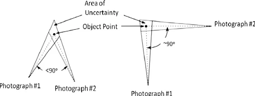
Figure 7. Minimising the area of uncertainty (source: Jiang & Jáuregui, 2010)

Jiang & Jáuregui (2010) also state that another basic principle governing camera placement and orientation is to ensure that the angle between the optical axes of the cameras is close to a right angle. Conducted either using a single camera from two different stations, or two camera capturing the image at the same time from the two different station, the area of uncertainty around the point of interest is minimised (refer to Figure 7 above). It would be advantageous to attain a third shot from another plane perpendicular to the first two, further reducing this area of uncertainty (Jiang & Jáuregui, 2010).

Mills & Barber (2004) suggest that two principle network configurations can be used to determine three dimensional coordinates from photogrammetric images. Figure 8 outlines these two configurations. The first network is that of a stereo network, commonly used to interpret aerial photography, but can be used to determine the three dimensional coordinates on an object of interest. The second configuration is that of the multistation convergent network, where an object is surrounded by a number of stations and images acquired and processed to produce a three dimensional image of the object.

Because more than two images are used, there are greater observational redundancies, improving accuracy, precision and reliability (Mills & Barber, 2004), and is therefore the primary configuration used to undertake the self-calibration technique and associated bundle adjustment for the self-calibration of non-metric cameras.

Single camera measurement

The primary purpose of photogrammetry is to determine the three dimensional coordinates of objects for the purposes of measurement. Because single camera measurements use a single camera, the reconstruction of three dimensions objects utilising single camera measurements requires significant additional geometric information (Luhmann et al. (2006). Typically applied for rectifications (Luhmann et al. (2006), Jiang et al. (2008) and Thomas & Cantré (2009) report that single camera setup uses the principle that if the camera image and object planes are parallel the actual dimension of an object will be directly proportional to that measured in the image.

software packages and would therefore require significant additional manual work in order to achieve sufficient adjustment resolution.

Stereophotogrammetric measurements

Stereo imagery is acquired where an automated stereoscopic image compilation process is used (Luhmann et al., 2006) to process the images, such as the

Australis software package. The process of stereoscopy provides that a point of interest on an object can be seen from another image taken from another camera located at a different station. To ensure that this can be achieved, Luhmann et al.

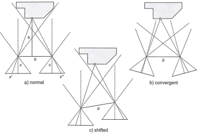
(2006) suggests that there are three camera positions that stereoscopy can be achieved (refer to Figure 9); the normal configuration (Figure 9a) where the two camera stations are located parallel and equidistant from the object of interest, and able to locate the same target from two different camera station images; shifted configuration (Figure 9c) where the cameras, while parallel to the object are at different offset, thereby requiring different scales to be applied to the image during the software processing; and convergent configurations (Figure 9b) where a greater angle of convergence than that of the human vision can be used to obtain the stereoscopic images.

Fraser (2001) and Mills & Barber (2004) warn that stereoscopic geometry can produce an inhomogeneous precision in the z axes (poor depth precision) and is largely dependent on the height to base ratio (Luhmann et al., 2006). This will require pre-planning to determine the exact requirements and tolerances of the photogrammetric project to account for this potential problem.

Multistation convergent networks

The number of camera stations and viewing directions are not restricted when using a multistation convergent network, with an object being acquired by an unlimited number of images to enable sufficient intersecting angles of bundles of rays in object space (Luhmann et al., 2006). Mills & Barber (2004) and Jiang et al. (2008) state that because of the amount of images that can potentially be used in the multistation configuration, the superior network design offered has a larger observation redundancy which improves accuracy, precision and reliability. This reliability ensures that uniform object accuracies in all coordinate directions can be attained (Luhmann et al., 2006).

Figure 8 indicates the basic multistation convergent network layout; the majority of close-range photogrammetric application utilise this configuration. This is especially so where a number of different viewing locations are required to capture areas otherwise occluded by the structure/shape of the object, or to meet the specified project requirements (Luhmann et al., 2006). Further, it is the multistation convergent network that best allows for the simultaneous calibration of cameras by self-calibrating bundle adjustment procedures (Luhmann et al., 2006) within an accepted photogrammetric software program.

2.6.3 Camera sensors

The first of the sensors is a charged coupled device, or CCD. This sensor consists of an array of photosensitive pixels that capture the light coming into the camera through the lens and then stores that information of the array as an electric charge Litwiller, 2001). Teledyne Dalsa (2011) reports that this charge is then converted to voltage before being passed on as an analog signal. This signal then gets converted into a digital image outside of the sensor.

The second sensor, the complementary metal oxide semiconductor (CMOS) sensor works similarly, except that each pixel (as opposed to the array of pixels) processes the light within each pixel (Litwiller, 2001) before the signal is output as a digital signal. This chip has numerous other components attached that allow this process to occur, but requires less off-chip processes to achieve the same operation as the CCD.

3

Research design and methodology

3.1

Laboratory testing

The laboratory testing and results is the subject of a research project conducted by Mr. Daniel Pratt for his undergraduate thesis. Specific testing and results will not be discussed, however a broad overview of his methods and results will be commented on.

3.1.1 Materials and equipment

To undertake the laboratory testing, consideration was given to the types of structures likely to be monitored and the materials that those structures may be constructed with. However, due to the size of the test area and the testing machine used in the laboratory photogrammetric work, test materials could only be representative of those used in structure construction. As such the materials tested consisted of timber railway sleeper, steel square-section, concrete, and fibre composite beams. In addition, a C-section guardrail post was included in the testing regime.

Targets used during the laboratory testing comprised of retro-reflective targets and non-reflective (diffuse) paper targets. The retro-reflective targets consisted of a black, commercially produced adhesive tape cut into a number of 10mm squares. Central to these squares was a retro-reflective circle, approximately 1.6mm in diameter. The diffuse targets consisted of a white, 10mm paper square, with a 3.2mm diameter black circle located centrally in the white square. These targets were glued to the beams in semi-random positions, as well as upon the universal testing machine.

Pre-testing pressure was applied to the beams to determine likely pressures that may indicate beam deformation. To this end, it was determined that the test pressures applied to the beams were:

• Timber: 0kN, 25kN, and 45kN.

• Concrete: 0kN, 7kN, and 13kN.

• Glass polymer resin: 0kN, 5kN, and 9.5kN.

• Steel square section: 0kN, 25kN, and 42.5kN.

• Steel C-section: 0kN, 25kN, and 45kN.

The cameras used to undertake the laboratory (and subsequent field) testing were Sony HDR-SR10 video cameras with CMOS image sensor and night vision capability. With a still picture resolution of 4 megapixels, photographs are produced in *.jpeg format. For night vision images, a Sony HVL-HIRL video infrared light was attached to the interface shoe located at the top rear of the camera unit. The IR emitter had a variable intensity switch to allow for an intensity to be matched to the conditions in which the camera and IR emitter is being used.

3.1.2 Control points and camera calibration

To ensure that the calibration board used for the camera calibration and additional control in the photogrammetric work has precise horizontal and vertical coordinates, an Anhui dissection control plate was employed. Further, a calibration scale bar with a known and precise length between the retro-reflective targets either end of the control rod. The calibration process for the large calibration board was processed in a similar manner to that of the photogrammetric images.

3.1.3 Image capture and processing of acquired images

Following calibration, a series of single images of each of the beams, under various load pressures, were captured. Sufficient overlap of the images ensured that stereoscopic photos could be produced. Images, once captured, were imported into the Australis v.6 software program for processing. Camera parameters used in the software processing can be found in Table 2 (refer to Section 3.2.3).

The laboratory processing and subsequent results, form part of the Research Project conducted by Mr Daniel Pratt. As such, little further discussion will occur within this Research Project, and will thus be saved for his discussions.

3.2

Field testing

3.2.1 Structure selection

A number of structures in the Darling Downs region of Queensland were examined for suitability in conducting field testing of conventional and infrared photogrammetry. Structural and positional aspects considered desirable were primarily the location with respect to Toowoomba, size of the structure, traffic volume, access to the structure, and site safety. The structure considered to meet these criteria was the Eton Vale Bridge, approximately 16.5km southwest of Toowoomba.

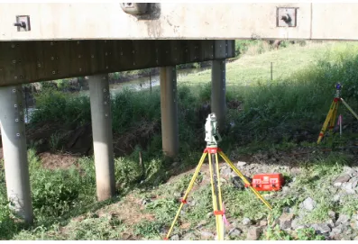
Constructed in 1969, the Eton Vale Bridge is described on the construction plans as a prestressed slab deck concrete bridge. With dimensions of 188’4” (36.088m) long and 28’ wide (8.534m), the overall deck unit consist of 70 prestressed girders and 10 prestressed kerb units. Supporting these girders and kerb units are four piers, each pier containing 5 x 16” (0.406m) hollow-spun piles driven to refusal. The pier headstock is nominally 2’6” (0.792m) in height; the targets used in the field testing are fixed to pier headstock number 4, and the associated piles.

Figure 10. The Hodgson Ck bridge at Eton Vale.

3.2.2 Establishment of control

Control traverse

during a recent traverse prior to construction works in the vicinity of the bridge site.

Between the datum marks, a number of secondary survey stations were established as part of the traverse. These stations were observed using the Leica TCRP1203+ ‘Sets of Angles’ program. Parameters used in the program allowed for a round of six face left/face right reciprocal readings to each of the stations to obtain horizontal and vertical coordinates for each station. Of importance to the bridge target location, two stations (Stations 3 and 4) were established approximately 3.5m adjacent to the piles and pile headstock to which the targets were attached.

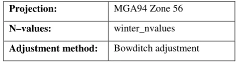
The survey program 12d (ver. 9.1) was used to process the traverse data. Utilising this program, reduction of the field data was conducted using the parameters contained in Table 1. The 12d report file for the control traverse, and the coordinates of the stations, can be found in Appendix B.

Table 1. Main parameters used in the 12d data reduction process.

Projection: MGA94 Zone 56

N–values: winter_nvalues

Adjustment method: Bowditch adjustment

For the purposes of this research project, the reduced levels (RL’s) of the secondary survey stations have remained with trigonometric heighting only; it was considered that as the two datum marks have spirit-levelled values, and that the traverse is relatively short in length with few stations contained on the traverse line, trigonometric heights will be sufficient to calculate target RL’s.

Target construction, placement and co-ordination

second type of target is a retro-reflective target, constructed of a ¾” (19.05mm) hollow-punched retro-reflective tape (3MTM Scotch® Reflective Tape 198DCNA, 25mm x 1m, 12/cs) glued to a 40x40mm black cardboard square.

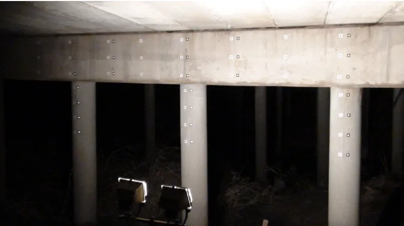
Consideration of target placement was undertaken to ensure sufficient coverage of the structure given its size and constructed material. For vertical positioning, it was decided that the pier headstock would contain three rows (A-C) of targets and that the piers would contain four rows (D-G) of targets. Horizontally (left-to-right) and based on the dimensions of the structure, it was decided that there would be 21 columns of targets; the total number of targets are 106. Figure 11 (below) is an example of the location of the targets on the structure.

Figure 11. An example of the target placement and location on the Hodgson Creek bridge pier headstock.

targets were measured similar to that of the headstock, with row D approximately 100mm below the pier/headstock intersection and spaced at approximately 250mm intervals. The total vertical height from row A to G is approximately 1.5m.

Horizontally, a mark was made approximately 750mm offset left and right of the pier centreline on the headstock, and a plumb line drawn from this mark. Where there are two types of targets (diffuse black circle and retro-reflective circle; refer to Figure 11) a mark 50mm offset left and right offset of the centreline was made for the location of the target. Once markout was completed, the concrete was cleaned of debris and the targets were secured to the piers and pier headstock using Selleys Liquid Nails construction adhesive.

Following target placement, the targets were located using the Leica TCRP1203+ instrument, and the onboard ‘Survey’ program. The instrument was set up on Station 3, and using the reflectorless EDM measurement mode, targets A100 through to G109 were manually sighted and measured. The instrument Station was moved to Station 4 and targets A110 through to G121 were measured as before. This data was then downloaded and processed in the 12d survey package where a report file indicating the coordinates of the targets was generated. This file can be found in Appendix C.

3.2.3 Image capture and processing of acquired images

The cameras used to undertake the target acquisition were the same as those used to undertake the laboratory testing (refer to Section 3.1.1). Given the width of the structure, it was considered that four different camera locations were required to provide sufficient coverage and overlap between photographs and ensure stereoscopy for processing. These locations were approximately 6m to the front of the pier and headstock, and approximately 4m apart – 2 locations at either side of the bridge, and 2 locations equidistant apart underneath the structure.

Figure 12. Target acquisition under bright light conditions.

From each location, four photographs were taken. The photographs were alternated between bright light (supplied by external floodlights powered by a portable generator) and total darkness. An example of this can be seen in Figure 12 and Figure 13, where the differences in illumination method (for the same photograph) are apparent. The photographs were captured in the following order – bright light (first direction), near infrared (first direction), bright light (second direction), near infrared (second direction), change of location. This process was repeated until all four locations had all four series of photographs captured.

for processing. The camera parameters (Interior Orientation parameters), required to process the photographs, are contained in Table 2. These parameters were established as part of the camera calibration conducted prior to the laboratory testing.

Figure 13. Target acquisition under total darkness utilising the infrared emitter attached to the camera.

Table 2. Camera parameters used in the Australis software processing.

Camera 1

(Light)

Camera 2

(Light)

Camera 1

(NIR)

Camera 2

(NIR)

Sensor size (mm) 2304 x 1296 2304 x 1296 2304 x 1296 2304 x 1296

Pixel size (mm) 0.00118 0.00118 0.00118 0.00118

Focal length(c) 3.041450 3.037979 3.040440 3.046335

(Xp) 0.002411 0.004786 0.001563 0.004673

(Yp) 0.002904 -0.001954 -0.007710 -0.003862

(K1) -3.0268x10

-3

-1.1555x10-3 -2.2043x10-3 1.0704x10-3

(K2) 3.3475x10

-3

1.5128x10-3 2.6412x10-3 -1.1954x10-3

(K3) -1.8291x10-3 -1.2679x10-3 -1.7789x10-4 8.6875x10-4

(P1) -1.6641x10-27 -3.66208x10-27 -1.0474x10-27 -1.6979x10-27

(P2) -2.2309x10

-27

-3.9374x10-27 -1.9807x10-27 -1.7375x10-27

(B1) -1.4199x10-28 -1.5735x10-28 3.5849x10-28 -1.4821x10-28

(B2) 3.4252x10-29 4.1154x10-30 6.6675x10-29 -1.0567x10-29

Referring to Table 2 and Table 3: Xp, Yp: Principal point offsets

P1, P2: Decentering distortion

B1, B2: Affinity and shear parameters

Additional photographs were taken at the bridge site using a Sony Cybershot DSC-F828 digital still camera, capable off taking photographs with a CCD-type sensor and an 8MP resolution. For this series (of photographs), the number of photograph stations was increased from four to five (corresponding with the number of pier piles), with up to eight colour and eight near-infrared photographs taken at each station. Assuming eight photographs were taken at each station, four were captured at a different height to the other four, separated by a minimum of 0.5m. Sufficient overlap to obtain stereophotographs at each station occurred, similar to the original photogrammetric process described previously.

Table 3. Camera parameters used in the Australis software processing for the additional photographs.

Camera 1

(Light)

Sensor size (mm) 3264 x 2448

Pixel size (mm) 0.0027

Focal length(c) 7.376340

(Xp) -.0.028995

(Yp) -0.077898

(K1) 2.9806x10-3

(K2) -1.5919x10

-5

(K3) -8.8082x10

-7

(P1) -2.3624x10-27

(P2) -5.6781x10

-28

(B1) 3.7057x10

-28

(B2) 5.8255x10-28

Once the control and driveback files (the same control file but with a different function during the processing) had been imported to the project, the photographs were imported and the digitised. This digitising process allowed for each individual target to have a unique identification number attached to it; this number is directly related to the number assigned to the target during the total station observations as outlined in Section 3.2.2. The correct assignment of the target number during the digitisation process is essential so that overlapping photographs with corresponding target numbers are recognised during the adjustment process of the software.

4

Results

Discussions with Mr. Daniel Pratt, and examination of the results obtained from the laboratory testing, suggest that there is no significant difference between conventional (colour) photogrammetry and near-infrared photogrammetry in the laboratory setting. The results suggested that there is between 0.1mm-0.3mm difference between the two photogrammetric methods (conventional v near-infrared). These laboratory results would then suggest that the expected accuracies of near-infrared photogrammetry are the same as, or at accuracies that can be described as the same, as that of conventional photogrammetry.

4.1

Background relating to the results

So that comparisons can be made and any differences between target types and photogrammetric methods can be identified, it was necessary to reduce the data into a single, simple measurement value. To do this, it was considered that the 3D distance was the best way to represent such data. Equation 1 (below) outlines the formula used to undertake the distance reduction used in the comparison between photogrammetric methods.

(

)

(

)

(

)

2 1 2 2 1 2 2 1

3 X X Y Y Z Z

d _D = − + − + − (1)

where:

X1, X2 = Easting value for the control and target type respectively

Y1, Y2 = Northing value for the control and target type respectively

Z1, Z2 = Northing value for the control and target type respectively

had the mean value of all distances reported. The method of calculation for the mean value is outlined in Equation (2).

n x x x

X ₌ 1 + 2 +... n

(2)

where:

X = mean value

xn = observed difference between the two identical target type

n = number of observa