A Novel Classification Technique for Visual
Evoked Potentials Based on Spectral Features
using Neural Network
Sarojini B.K1, Dr.Basavaraj S.Anami2, Dr.Mukartihal G.B3 , Kotresh.S4
Professor, Dept. of ECE, Basaveshwar Engineering College, Bagalkot, Karnataka, India1
Principal, K.L.E.Institute of Technology, Hubballi, Karnataka, India2
Professor & Head, Dept. of EEE, Basaveshwar Engineering College, Bagalkot, Karnataka, India3
Associate Professor, Dept.of EEE, Rao Bahadur Y Mahabaleshwarappa Engineering College, Ballari, Karnataka, India4
ABSTRACT: It is important to differentially diagnose Optic neuropathy (ON) and Ischemic optic neuropathy (ION) diseases for prognostic and therapeutic purposes. Generally, differentiation is accomplished by assessing the disc appearance, presence / absence of retrobular pain, patient’s age, mode of onset and other parameters of clinical and laboratory evaluation. However, in some patients, diagnosis may be difficult because of overlapping clinical profiles of these two disorders. In routine clinical practice, differentiation of ON and ION is accomplished by neurologist assessing recorded visual evoked potentials (VEPs) of a patient in only time domain, which is primarily concerned with P100 latency and its peak.
In this paper, an attempt is made to overcome the difficulty of clinically overlapping profiles. A multilayer neural network model is developed with spectral features as the input vector and normal, ON & ION are the target outputs. Thismodel was trained using back propagation algorithm and tested with variable nodes in both hidden layers. For a typical structure 6L: 30N:5N:3N the training error has been reduced significantly after about 100 epochs. This model has the potential to differentiate ON and ION with respect to normal subjects. Classification accuracy is computed using confusion matrix and found to be 83.33%. This novel technique is objective, hence overcomes clinically overlapping profiles of ON and ION diseases thus enables the neurologist in early therapy planning.
KEYWORDS: Visual evoked potentials, Neural network, Back propagation algorithm, Confusion matrix, Classification accuracy.
I. INTRODUCTION
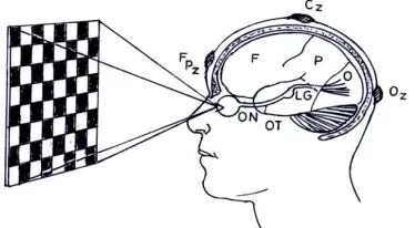
Evoked potentials (EPs) are bioelectric signals generated by the central nervous system (CNS) when it is stimulated by well defined external events. The most commonly used clinical EPs are the checkerboard visual evoked potentials (VEPs), the brain stem auditory evoked potentials (BAEPs), and the median & posterior tibial nerve somatosensory evoked potentials (SEPs) [1]. VEPs are electrical potential differences produced by the electrical activity of visual cortex in response to visual stimuli. These potentials are generated in the posterior part of occipital lobe. VEPs are used in a variety of clinical applications. These include estimation of optic nerve function, estimation of visual acuity in infants, in young children and adults unable to provide reliable verbal responses, in detection of malingering, and assessment of amblyopia [2].
therapeutic reasons. ON is a severely blinding disease resulting from loss of the arterial blood supply to the optic nerve as a result of occlusive disorders of the nutrient arteries. ION is characterized by painless, irreversible and nonprogressive loss of vision accompanied by nerve fiber bundle type of defect, an afferentpapillary defect and disc oedema. In clinical practice, diagnosis is accomplished by the signs and symptoms, and other features of clinical and laboratory tests. However signs and symptoms of these two disorders overlap in certain group of patients, making differential diagnosis difficult for the neurologist. Clinically relevant parameters of VEP, namely, absolute and interwave latencies, interside latency difference, amplitudes and amplitude ratios have to be analyzed from the sample in differentiating normal and diseased subjects [3]. Comparative studies on pattern visual evoked cortical potentials to differentiate ON from ION using clinical and laboratory tests is available in the literature [4]. However, in certain group of patients, diagnosis may be difficult because of overlapping clinical profiles in these two conditions. To circumvent this problem, neural network modeling is proposed in this paper for the effective classification of ON and ION disease groups with respect to normal subjects based on the extracted spectral features of VEP.
II. RELATED WORK
Spectral analysis technique has been used with rectangular and Kaiser windows for the analysis of VEPs in order to differentiate normal and Alzheimer groups. It has been found from the study, that Kaiser window is the most effective in correct classification of all normal and Alzheimer’s diseased patients [5]. A new algorithm called subspace averaging is developed for performing signal averaging on VEPs. This algorithm yielded higher signal to noise ratio (SNR) relative to the conventional ensemble averaging [2].
The effect of alcohol on central nervous system (CNS) of human beings has been studied using VEPs. It is reported that the alcoholics suffer a kind of irreversible alteration in the brain even after quitting alcohol [6]. A new approach based upon the adaptive chirplet transform (ACT) has been proposed to characterize the time – dependent behaviour of the VEPs. This approach demonstrated that the adaptive Chirplet spectrogram (ACS) yielded a better visualization of VEP decompositions as compared to the traditional, short – time Fourier transform (STFT) based spectrogram [7].
III.METHODOLOGY
Detailed methodology employed in this work is described in the sub-sections to follow one after another.
A. Materials and Methods
Recording of VEPs is done routinely in clinical practice using a typical electrodiagnostic test setup. The eyes of the subjects are tested one at a time while the other eye is covered with an eye patch. Standard nomenclature has been adopted for describing the VEP waveform. The usual convention is that upward deviation caused by an impulse relative to reference is defined as negative. Waveforms of VEP are named by their polarity (P or N) followed by their latency (often indicated by a bar over the number). Latency is defined as the time interval between the onset of a controlled stimulus and a selected peak in VEP signal. Important features of the VEP, namely, latency and amplitudes are measured because of their significant relevance in electro-physiological diagnostics in neurology and neuro-ophthalmology. In clinical practice, the amplitude between the first positive peak P100 and the preceding negative trough N75 and the peak latency of the P100 component are measured. Reduced amplitudes and prolonged latencies in comparison with those of healthy controls are reliable indicators for pathological changes in visual pathways [8].
B. Subjects
C. Electrode and Electrode Placement
Standard silver-silver-chloride, disc type surface electrodes of 10 mm diameter, 1.5 m lead lengths were employed for recording VEPs. The electrode site was prepared by rubbing with a cotton swab dipped in an abrasive skin prepping Gel (NuprepTM ). The electrodes were filled with Ten20TM conductive EEG paste and held in place on the scalp using 3M micro pore adhesive tape. The electrode impedance was less than 5 k. Electrodes were placed relative to bony skull landmarks, in proportion to the size of the head, according to the International 10/20 system of EEG electrode placement configuration [11]. The ground electrode is placed on the forehead (Fpz). The measuring and reference electrodes are placed on the scalp over the visual cortex (Oz) and on the vertex (Cz), respectively, as shown in Figure 1.
Figure.1 Schematic of VEP Recording
D. Signal Acquisition
All VEP recordings were performed in a dark and sound attenuated room in the neuro-diagnostic laboratory of Vijay Health Centre, Chennai. Subject was asked to sit comfortably in front of the checkerboard pattern at an eye-screen distance of 100 cm. The stimulus pattern was a black and white checkerboard displayed on a Sanyo B/W video monitor, with individual checks subtending 2.29˚ and the entire pattern 18.32˚ at the eyes of the subject. The checks alternate
from black/white to white/black at a rate of approximately twice per second [12]. The subject was instructed to gaze at a colored dot on the centre of the monitor screen. Every time the pattern alternates, the patient’s visual system generates an electrical response and was recorded using electrodes. Signal acquisition and stimulus presentation was controlled by Cadwell Sierra - II Electrodiagnostic test setup, with filter settings at 1-100 Hz. The starting point of VEP waveform is stimulus onset. The VEP waveform recording is done over a period of 250 ms. More than 100 epochs were averaged to ensure a clear VEP waveform. For judging the reproducibility, the waveform is recorded twice and superimposed. A typical averaged VEP waveform is shown in Figure 2.
E. Digitization and Feature extraction
Every recorded VEP waveform from 0 to 250 ms is digitized using Grafula software with an inter-sample interval of 0.66 ms, thus providing 375 digital data sequence. The digitized VEP signals were transformed into frequency domain using fast Fourier transform (FFT) implemented in MATLAB. Power spectra were constructed by computing the magnitude squared of each discrete frequency component. Typical power spectrums of the recorded VEP signals for normal, ON and ION patients are shown in Figure 3(a), 3(b) and 3(c)respectively.
0 10 20 30 40 50
0 5 10 15 20 25 30 35
Frequency in Hz
P
o
w
e
r
in
V
2 /H
z
Figure. 3(a) Power spectrum of Normal
0 10 20 30 40 50
0 5 10 15 20 25 30 35
Frequency in Hz
P
o
w
e
r
in
V
2 /H
z
Figure. 3(b) Power spectrum of ON
5 10 15 20 25 30
P
o
w
e
r
in
V
2 /H
First three dominant frequency components (f1, f2, f3) and corresponding powers (p1, p2, p3) of the power spectra are the extracted spectral features. From the power spectra of normal, ON and ION, it is observed that with respect to normal, the first dominant peak is characterized by low frequency and high power for ON subject whilst high frequency and low power for ION subject.
IV.NEURAL NETWORK TOPOLOGY AND PERFORMANCE ESTIMATE
Neural networks (NN) are a compact group of connected, ordered in layer elements able to process information. NN based approaches have the advantages of self learning and ability to model complex data without need for a detailed understanding of the underlying phenomenon. NN can be described as mapping an input space to an output space.
A. Neural network modeling in optic nerve diseases
Developing an NN based classifier requires addressing several issues, such as deciding which type of NN to use, choosing the NN architecture and selecting the cost & activation functions. Although, a minimal NN has only two layers of nodes input and output; the most widely used are slightly more complicated, comprising at least three layers: input, hidden (one or more) and output. The optimal structure plays an important role while using neural network model for classification. The input layer neurons receive data from a data file. The output neurons provide NN’s response to the input data. The function of hidden neurons intervene (interface) between the external input and the network output in some useful manner. A feature selection allows the optimization of the number of neurons in the input layer. However, according to the Ockham’s Razor principle (also called the principle of economy), it must be as reduced as possible, because too many free parameters in the NN allows the network to fit the training data arbitrarily closely (over fitting) but does not lead to an optimal generalization.
Figure. 4 Four layer feedforward neural network model
This model has full interconnection from the input nodes to the hidden nodes and to the output nodes. The most popular node function used in NN is “sigmoid” (S-shaped) function because it has nice mathematical properties such as monotonicity, continuity and differentiability, which are very important when training a neural network with gradient descent method [14]. The bipolar sigmoid function is used both for the hidden and output nodes. Mathematically, sigmoid function is defined by:
)
2
tanh(
)
1
(
)
1
(
)
(
x
e
e
x
f
x x
where, tanh denotes hyperbolic tangent. The limiting values of this sigmoid function are: -1 and +1.
In the back propagation learning algorithm, the input is first propagated through the network and calculates the output.
Then the error between the desired output and the actual output, called the cost function (ξ), is propagated backward
from the output to the input to adjust the weights. The weight update functions (WUFs) play an important role in the reliability of the models using NN. The Levenberg-Marquardt algorithm was shown to be the best WUF. Mathematically, the algorithm minimizes the cost function with a gradient descent method [15, 16].
Learning rate (α) which determines the rate of convergence should be neither too low nor too high. It improves the
gradient descent in the positive direction without much oscillation. To avoid oscillation to extreme values during learning, a small constant η (momentum) is added to gradient descent to smoothen it’s path towards the positive
direction and also to improve the convergence rate. Generally, the η value 0.5 – 0.9 is used that allows faster learning
rate without much oscillation. In the present work, learning rate α = 0.2 and momentum η = 0.9 are adopted.
For classifiers, the outputs are generally coded with a +1 for existence in that class and -1 for absence from that class. For sigmoidal output neurons, sometimes, the target output values are pushed back from the extreme edges of the sigmoid so that 0.9 and - 0.9 for hyperbolic tangent function are used instead [14].
The training data consists of a number of patterns belonging to each class. The aim of training is to form decision surfaces among the regions of all the classes in the pattern space. Generally, 70% of the available patterns with output are used for training and 30% of the patterns are used for testing (the percentage may vary and is not the thumb rule for training) [17].
B. Performance Estimate
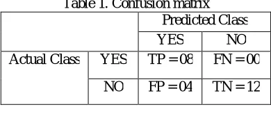
True Positives (TP) - number of subjects correctly classified as healthy; True Negatives (TN) - number of subjects correctly classified as abnormal;
False Positives (FP)- number of subjects misclassified as normal when actually abnormal; False Negatives (FN) -number of subjects misclassified as abnormal when actually normal [18].
The performance of the proposed model is evaluated by computing the percentage of correct classification accuracy. Mathematically, the classification accuracy is given by the following expression:
Classification accuracy (AC) =
FN
FP
TN
TP
TN
TP
In the classification problems, the purpose of the network is to assign each case to one of the classes. Keeping track of all these possible outcomes is such an error-prone activity, that they are usually shown in what is called a confusion matrix. The details of confusion matrix are summarized in Table 1.
Table 1. Confusion matrix Predicted Class
YES NO
Actual Class YES TP = 08 FN = 00
NO FP = 04 TN = 12
V. RESULTSANDDISCUSSION
Training is carried out until the total sum of mean squares error reaches the desired error value of 0.0001 or till the completion of desired number of epochs. The different networks are trained for varying size of the nodes in the hidden layers. Figure 5 shows the trend in training error for each epoch. For a typical structure 6L:30N:5N:3N the training error has been reduced significantly after about 100 epochs.
0 10 20 30 40 50 60 70 80 90 100
0 0.2 0.4 0.6 0.8 1 1.2 1.4 1.6 1.8
Figure. 5 Training error curve for 100 epochs X-axis: Number of epochs Y-axis: Mean squared error
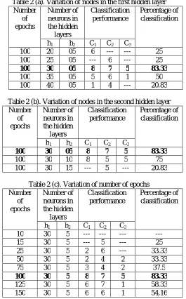
Table 2 (a). Variation of nodes in the first hidden layer Number
of epochs
Number of neurons in the hidden
layers
Classification performance
Percentage of classification
h1 h2 C1 C2 C3
100 20 05 6 --- --- 25
100 25 05 --- 6 --- 25
100 30 05 8 7 5 83.33
100 35 05 5 6 1 50
100 40 05 1 4 --- 20.83
Table 2 (b). Variation of nodes in the second hidden layer Number
of epochs
Number of neurons in the hidden
layers
Classification performance
Percentage of classification
h1 h2 C1 C2 C3
100 30 05 8 7 5 83.33
100 30 10 8 5 5 75
100 30 15 --- 5 --- 20.83
Table 2 (c). Variation of number of epochs Number
of epochs
Number of neurons in the hidden
layers
Classification performance
Percentage of classification
h1 h2 C1 C2 C3
10 30 5 --- --- --- ---
15 30 5 --- 5 --- 25
25 30 5 2 6 --- 33.33
50 30 5 2 4 2 33.33
75 30 5 3 4 2 37.5
100 30 5 8 7 5 83.33
125 30 5 6 7 1 58.33
150 30 5 6 6 1 54.16
It is seen from Table 2(a) that better classification is achieved for 30 nodes in the first hidden layer (h1). Also, from Table 2(b) it is evident that 5 neurons in the second hidden layer (h2) yields better performance. From Table 2(c), it is observed that the better performance is achieved when the numbers of neurons in the first and second hidden layers are 30 and 5 respectively for 100 epochs.
been decreased. This can be observed from last column of Table 2(c). When the number of iterations are about 10, the model has not learnt behavior of the examples properly, which can be seen from first row of Table 2(c).
In the present study, the values of TP, TN, FP, and FN obtained are 8, 12, 04, and 00 respectively. Classification accuracy is computed using confusion matrix and it is found to be 83.33%. Thus, the network structure 6L:30N:5N:3N is the optimized model for classification of subjects into normal, ON, and ION groups.
VI.CONCLUSION
In routine clinical practice, diagnosis of ON and ION diseases performed by a neurologist, involves visual inspection of the VEP waveform, which is primarily concerned with only time domain parameters of P100 latency and its peak amplitude. Visual interpretation is not only subjective, but also depends more upon personal skills and hence does not lend itself to statistical analysis. Therefore, quantitative VEP analysis method based on advanced digital signal processing techniques would be of great value for neurologist in deciding a therapy.
To circumvent the difficulties associated with prevailing practice, a multilayer NN model is developed with spectral features as the input vector while normals, ON, and ION are the target classes. Extraction of spectral features involves the overall composition of the VEP waveform otherwise not disclosed by P100 latency and its peak measurements. The developed NN model was trained with back propagation algorithm and varying nodes in both the hidden layers. It is clear from the earlier section that for 100 iterations (epochs), the topology corresponding to 6L:30N:5N:3N resulted in optimum performance. With this architecture, VEPs recorded over a number of patients and normals were able to be classified as normals, ON, and ION to an accuracy of 83.33 percent using confusion matrix.
Suffice it to conclude that NN modeling described herein, is objective and is free from interpersonal variations. Hence, it enables the neurologist in diagnostic and prognostic approach thus overcoming the drawbacks associated with the conventional practices in vogue.
VII.ACKNOWLEDGMENT
The authors express gratitude to Dr.Sureshkumar and Dr.(Col) S.S.K.Ayyar, Consultants in Neurology and Clinical Neuro-physiology of Vijay Health Centre, Chennai for their extended support for providing relevant information regarding optic nerve diseases and in collection of VEP data.
REFERENCES
[1] Nuwer M.R “Fundamentals of evoked potentials and common clinical applications today”, Electroencephalography and Clinical Neurophysiology. 106, pp 142-148, 1998
[2] Davila C. E and R. Srebro“Subspace averaging of steady-state visual evoked potentials”. IEEE Trans. Biomed. Eng, 47, pp 720-727, 2000. [3] Chiappa H. K “Evoked Potentials in Clinical Medicine”, New York, Raven Press, 1999.
[4] Michihiko T. A. Mizota, and E. Adachi-Usami “Comparative studies on pattern VECP between patients with ischemic optic neuropathy and optic neuritis” Acta Ophthaalmol. Scand, 78, pp 407-410, 2000.
[5] Moody E.B., E. Micheli, and S. Chokroverty “An adaptive approach to spectral analysis of pattern – reversal visual evoked potentials”, IEEE Trans. Biomed. Eng, 36, pp 439-447, 1999.
[6] Palaniappan, R and P. Raveendran “Classification of single trial gamma based VEP extraction during object recognition”, Proceedings of the International Cconference on Biomedical Engineering Bangalore, pp 85-88, December 2001.
[7] Jie, C. and W. Wong “The adaptive chirplet trnaform and visual evoked potentials”,IEEE Trans. Biomed. Eng, 53, pp 1378- – 1384, 2006. [8] Pecher A. Husar P. Henning G, Roderer H. “Phase estimation of visual evoked responses.” IEEE Trans . Biomed. Eng. 50, pp 324-333, 2003. [9] Leif, S. and P. Laguna Bioelectrical Signal Processing in Cardiac and Neurological Applications. Elsevier Academic Press, London, 2005. [10] Mishra U. K, Kalitha J. “Clinical Neurophysiology-Nerve conduction Electromyography Evoked potentials”, 3rd Edition, Elsevier, New Delhi, 2015. [11] Jasper H. “Report of committee on methods of clinical exam in EEG” Electroencephalogr. Clin. Neurophysiol., 10, pp 370-375, 1958.
[12] Mitchell, B., B. Michael, B. Colin, M. Anne, and R. John “Guidelines for Calibration of Stimulus and recording Parameters Used in Clinical Electrophysiology of Vision” Revised ISCEV, 2009.
[13] Haykin S “Neural Networks and learning machines”. 3rd edition, PHI, New Delhi, 2011.
[14] Kevin L. Priddy and Paul E. Keller “Artificial neural networks an introduction”. PHI, New Delhi, Eastern Economy Edition, 2009. [15] David J. Livingstone “Artificial neural networks methods and applications”. Springer International Edition, Springer, 2011.
[16] Hagan. M.T, and Menhaj M. B. “Training Feedforward Networks with the Marquardt Algorithm”, IEEE Transaction on Neural Networks, Vol. 5, Issue 6, pp 989-993,1994.
[17] B. K. Tripathy and J. Anuradha “Soft computing advances and applications”. Cengage learning, 2015.