Comparison of LQR and PD controller for stabilizing Double Inverted Pendulum System

ISSN: 2278-067X, Volume 1, Issue 12 (July 2012), PP. 69-74

www.ijerd.com

Comparison of LQR and PD controller for stabilizing Double

Inverted Pendulum System

Narinder Singh

, Sandeep Kumar Yadav

Department of control and instrumentation Engineering, NIT Jalandhar, Punjab 144011 India

Abstract—

Keywords––

I.

INTRODUCTION

Te inverted pendulum offers a very good example for control engineers to verify a modern control theory. This can be explained by the facts that inverted pendulum is marginally stable, in control sense, has distinctive time variant mathematical model. The double inverted pendulum is a highly nonlinear and open-loop unstable system. The inverted pendulum system usually used to test the effect of the control policy, and it is also an ideal experimental instrument in the study of control theory [1, 2]. To stabilize a double inverted pendulum is not only a challenging problem but also a useful way to show the power of the control method (PID controller, neural network, FLC, genetics algorithm, etc.).

In this paper common control approaches such as the linear quadratic controller (LQR) and PD controller based on a pole placement technique to overcome the problem of this system require a good knowledge of the system and accurate tuning obtain good performance [3-5]. This paper presents investigations of performance comparison between modern control and PD control for a double inverted pendulum system. Performance of both controller strategies with respect to pendulums angle and cart position is examined.

II.

MODELING

OF

DOUBLE

INVERTED

PENDULUM

To control this system, its dynamic behavior must be analyzed first. The dynamic behavior is the changing rate of the status and position of the double inverted pendulum proportionate to the force applied. This relationship can be explained using a series of differential equations called the motion equations ruling over the pendulum response to the applied force. The double inverted pendulum is shown in Fig 1. The meanings and values of the parameters for inverted pendulum are given in Table 1. [4]

Fig1: schematic diagram of Double Inverted Pendulum

To derive its equations of motion, one of the possible ways is to use Lagrange equations [6]

𝑑 𝑑𝑡

𝑑𝐿 𝑑𝑞 𝑖

− 𝑑𝐿 𝑑𝑞𝑖

TABLE I :PARAMETERS OF DOUBLE INVERTED PENDULUM

M(m1,m2,m3) Mass of thecart,( first pole, second pole, joint)

5.8kg(1.5kg,.5kg,.75kg)

θ1,θ2 The angle between pole 1(2) and vertical direction (rad)

L1(l1), L2(l2) Length of pendulum first(2l1) and length of second pendulum (2l2) ,1m,1.5m

g Center of gravity 9.8m/s2

F Force applied to cart

Where L = T - V is a Lagrangian, Q is a vector of generalized forces (or moments) acting in the direction of generalized coordinates q and not accounted for in formulation of kinetic energy T and potential energy V. Kinetic and potential energies of the system are given by the sum of energies of cart and pendulums.

𝑇 = 1

2 𝑚0+ 𝑚1+ 𝑚2+ 𝑚3 𝑥 2₊ 2

3𝑚1𝑙1 2_{+ 2𝑚}

2𝑙12+ 2𝑚3𝑙12 𝜃 1 2

+1

6 𝑚2𝑙2 2_𝜃

2 2

+ 𝑚1𝑙1+ 2𝑚2𝑙1+

2𝑚3𝑙1 𝑥 𝜃 1𝑐𝑜𝑠 𝜃1+ 𝑚2𝑙2𝑥 𝜃 2𝑐𝑜𝑠𝜃2+ 2𝑚2𝑙1𝑙2𝑐𝑜𝑠 𝜃1− 𝜃2 𝜃 1𝜃 2 (2)

𝑉 = 𝑚1𝑔𝑙1cos𝜃1+ 2𝑚3𝑔𝑙1cos𝜃1+ 𝑚2𝑔(2𝑙1cos𝜃1+ 𝑙2cos𝜃2) (3)

Thus the Lagrangianof the system is given

𝐿 = 1

2 𝑚0+ 𝑚1+ 𝑚2+ 𝑚3 𝑥 2₊ 2

3𝑚1𝑙1 2_{+ 2𝑚}

2𝑙12+ 2𝑚3𝑙12 𝜃 1 2

+1

6 𝑚2𝑙2 2_𝜃

2 2

+ 𝑚1𝑙1+ 2𝑚2𝑙1+

2𝑚3𝑙1 𝑥 𝜃 1𝑐𝑜𝑠 𝜃1+ 𝑚2𝑙2𝑥 𝜃 2𝑐𝑜𝑠𝜃2+ 2𝑚2𝑙1𝑙2𝑐𝑜𝑠 𝜃1− 𝜃2 𝜃 1𝜃 2 − 𝑚1𝑔𝑙1cos𝜃1− 2𝑚3𝑔𝑙1cos𝜃1− 𝑚2𝑔(2𝑙1cos𝜃1+

𝑙2cos𝜃2) (4)

Differentiating the Lagrangian by and θ and θ yields Lagrange equation (1) as:

𝑑 𝑑𝑡

𝑑𝐿 𝑑𝜃 1

− 𝑑𝐿 𝑑𝜃1

= 0 (5) 𝑑

𝑑𝑡 𝑑𝐿 𝑑𝜃 2

− 𝑑𝐿 𝑑𝜃2

= 0 (6)

Or explicitly:

4 3𝑚1𝑙1

2_{+ 4𝑚}

2𝑙12+ 4𝑚3𝑙12 𝜃 1+ 𝑚1𝑙1+ 2𝑚2𝑙1+ 2𝑚3𝑙1 𝑥 cos𝜃1+ 2𝑚2𝑙1𝑙2𝜃 2𝑐𝑜𝑠 𝜃1− 𝜃2 + 2𝑚2𝑙1𝑙2𝜃 2 2

𝑠𝑖𝑛 𝜃1−

𝜃2 − 𝑚1𝑙1+ 2𝑚2𝑙1+ 2𝑚3𝑙1 𝑔 sin𝜃1= 0 (7)

𝑚2𝑙2𝑥 𝑐𝑜𝑠𝜃2+ 2𝑚2𝑙1𝑙2𝜃 1𝑐𝑜𝑠 𝜃1− 𝜃2 + 1 3 𝑚2𝑙2

2

𝜃 2− 2𝑚2𝑙1𝑙2𝜃 1 2

𝑠𝑖𝑛 𝜃1− 𝜃2 − 𝑚2𝑙2 𝑔 sin𝜃2= 0 (8)

Lagrange equation for the DICP system can be written in a more compact matrix form: D(θ) 𝜃 +C(θ,𝜃 ) 𝜃 + G(θ) = Hu (9)

The stationary point of the system is (𝑥, 𝜃1, 𝜃2, 𝑥 , 𝜃 1, 𝜃 2,𝑥 ) = (0, 0, 0, 0, 0, 0, 0), introduce small deviation around a stationary

point and Taylor series expansion; the stable control process of the Double Inverted Pendulums are usually cos(θ1 – θ2)=1, sin (θ1 – θ2), cos(θ1)≅cos(θ2)≅1, sin(θ1)≅θ1, sinθ2≅ θ2 . Linearization is made at balance position; we can get the linear time invariant state space model [7].

𝑥 𝜃 1

𝜃 2

𝑥 𝜃 1

𝜃 2

= 0 0 0 0 0 0 0 0 0 0 14.2545 −14.2545 0 0 0 0 −4.0090 21.1077 0 0 0 0 0 0 0 0 0 0 0 0 0 0 0 0 0 0 𝑥 𝜃1 𝜃2 𝑥 𝜃 1

𝜃 2

+ 0 0 0 1 1.1818 0.1818 𝑢(𝑡) 𝑦 𝑡 = 1 0 0 0 1 0 0 0 1 0 0 0 0 0 0 0 0 0 𝑥 𝜃1 𝜃2 + 0 0 0

𝑢(𝑡) (10)

III.

ANALYSIS

OF

DOUBLE

INVERTED

PENDULUM

After obtaining the mathematical model of the system features, we need to analyze the stability; controllability and Observability of systems in order to further understand the characteristics of the system [8].

A.

Stability

If the closed-loop poles are all located in the left half of “s” plane, the system must be stable, otherwise the system is unstable. In MATLAB, to strike a linear time-invariant system, the characteristic roots can be obtain by eig (a,b) function. According to the sufficient and necessary conditions for stability of the system, we can see the inverted pendulum system is unstable

B.

Controllability

A system is said to be controllable if any initial state x(t0 ) or x0 can be transfer to any final state x( tf) in a finite time interval (tf - t0), t ≥ 0 by some control u.

Qc = [B AB … … … … An-1B] (10)

C. Observability

A system is said to be observable if every state x0 can be exactly determined from the measurement of the output „y‟ over a finite interval of time 0 ≤ t ≥ tf.

The test of controllability due to Kalman if system is completely observable if and only if the rank of composite matrix is n where

Oc = [CT AT CT (AT )2CT……….(AT)n-1 CT] (11)

IV.

DESIGN

OF

LINEAR

QUADRATIC

REGULATOR

This leads to the Linear Quadratic Regulator (LQR) system dealing with state regulation, output regulation, and tracking. Broadly speaking, we are interested in the design of optimal linear systems with quadratic performance indices [9].

We shall now consider the optimal regulator problem that, given the system equation.

𝑥 (𝑡) = A x(t) + Bu(t)

Y(t) = C x(t) + D u(t) (12)

Determine the matrix K of the optimal control vector.

𝑢 𝑡 = −𝐾𝑥 𝑡 (13) So as to minimize the performance index J = (𝑥∞ 𝑇 _{𝑡 𝑄𝑥 𝑡}

0 + 𝑢

𝑇 _{𝑡 𝑅𝑢 𝑡 )𝑑𝑡 (14)}

Where Q is a positive-semi definite and R is a positive-definite matrix. The matrices Q and R determine the relative importance of the error. Here the elements of the matrix K are determined so as to minimize the performance index.

Then 𝑢 𝑡 = −𝐾𝑥 𝑡 = −𝑅−1_𝐵𝑇_{𝑃𝑥(𝑡) is optimal for any initial x(0) state.}

Fig 2: Full state feedback representation of DIP

Where P (t) is the solution of Riccati equation, K is the linear optimal feedback matrix. Now we only need to solve the Riccati equation.

𝐴𝑇 _{𝑃 + 𝑃𝐴 − 𝑃𝐵𝑅}−1_𝐵𝑇_{𝑃 + 𝑄 = 0 (15)}

Where Q and R chose as Q = diag ([10 60 80 0 0 0]) and R = 1. Therefore,

K= −𝑅−1_𝐵𝑇_{𝑃 = [10 275.2453 -515.6502 16.2044 22.1046 -111.9285]}

V.

DESIGN

OF

PD

CONTROLLER

A Proportional-Derivative (PD) controller is a control loop feedback mechanism used in process control type industrial. A PD controller calculates an “error” value as the difference between a measured process variable and a desired set point. The controller attempts to minimize the error by adjusting the process input. PD controller calculation involves two parameters values proportional (P) and derivative (D). Proportional values is determines the reaction to the current error, derivative values determines the reaction rate at which the error has been changing [5~10].

PD controller is combination of proportional plus derivative controller. It consists to a single input three output of a double inverted pendulum system. This is the case of stabilization of a double inverted pendulum at is x = 𝜃1= 𝜃2= 0,

which is a physical unbalance position. So integral action will result in instability condition of control system and a simple PD controller is more adaptive. Then we have used a three (multi) PD controller.

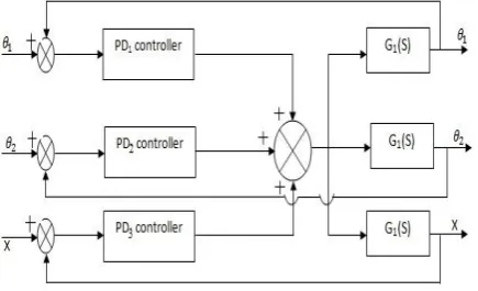
The transfer function of PD controller is (Kp + KdS) i.e. PD1, PD2, and PD3 transfer functions are respectively (K1 +K2S), (K3 +K4S) and (K5 +K6S).

Fig4: The structure of DIP PD controller

We now use a pole placement technique of state feedback control system to determine the 6 PD control parameter. When assume that desired closed pole are -2.1±2.1425j, -5, -5, -5, -5. We can obtain the parameter of PD controller by using the MATLAB i.e.

K1=131.4941, K2=-23.4289, K3=-549.4167 K4=-124.6183, K5=23.0785, K6=29.2327

VI.

SIMULATION

AND

RESULT

The system under consideration and the proposed controllers are modeled and simulated in the MATLAB/Simulink environment. The step response performance of the two controllers is compared fig.5 shows the step response of the system under consideration in absence of a controller and is found to be unstable.

Fig6: Step response of Pendulum angles and cart position by using LQR controller.

Fig7. Step response of cart position by using PD controller

Fig8: The response of first pendulum angle by PD controller

Fig9: The response of second pendulum angle by PD controller

TABLE2 Time response

specification

LQR controller

PD controller Settling time

(Ts)

3.05 s 3s

Rise time (Tr) 0.51s .15s

Peak overshoot 20% 5.8%

steady state error (ess)

0.02 0.0117

SUMMARY OF THE PERFORMANCE CHARACTERISTICS FOR CART POSITION

TABLE3 Time response

specification

LQR controller

PD controller Settling time

(Ts)

4.68S 2.876S

Rise time (Tr) 0.21S 0.17S

Peak overshoot 1.6% 7.5%

Steady state error (ess)

0 0

SUMMARY OF THE PERFORMANCE CHARACTERISTICS FOR FIRST PENDULUM‟S ANGLE

TABLE 4 Time response

specification

LQR controller

PD controller Settling time(TS) 4.67S 3.08S

Rise time (Tr) 0.907S 0.62S

Peak overshoot 5% 7%

Steady state error (ess)

0 0

SUMMARY OF THE PERFORMANCE CHARACTERISTICS OF SECOND PENDULUM‟S ANGLE

From both controller LQR and PD controller‟s result, It is clear that both are successfully designed but PD controller exhibits better response and performance.

VII.

CONCLUSION

In this paper, LQR and PD controller are successfully designed for a Double Inverted Pendulum system. Based on the results, both controllers are capable of controlling the double inverted pendulum‟s angles and the cart position of the linearized system. However, the simulation result shows that PD controller has a better performance as compared to the LQR controller in controlling the Double Inverted Pendulum system.

REFERENCES

[1]. Yan xueli, JIANG hanhong. “Control method study on a single inverted pendulum in a simulink environment”. Measure and

control technology, 2005, 24(07):37-39.

[2]. ZHAN G Hongli “simulation of virtual inverted pendulum based on MATLAB”. Machine Building and Automation, Dec

2004,33(6):103-105

[3]. Chen Wei Ji, Fang Lei, and Lei Kam Kin, “Fuzzy logic controller for an inverted pendulum,” system and control in Aerospace and Astronautics, 2008. ISSCAA 2008. 2nd _{international symposium on, vol.,no.,pp.1-3,10-12 Dec 2008.}

[4]. Gugao Company, GT-400-SV inverted pendulum users’ guide. 2002.

[5]. Yingjun Sang, Yuanyuan Fan, Bin Liu, “double inverted pendulum control based on three loop PID and improved BP neural network,” second international conference on digital manufacturing & Automation,2011,456-459.

[6]. Bogdanov Alexander, 2004, “Optimal Control of a Double Inverted Pendulum on a Cart”, Technical Report CSE-04-006.Y.

[7]. A.L. Fradkov, P. Y. Guzenko, D. J. Hill, A. Y. Pogromsky. “Speed gradient control and passivity of nonlinear oscillators,”

Proc. of IFAC symposium on Control of Nonlinear Systems, Lake Tahoe. 1995:655-659.

[8]. Jian Pan, Jun Wang “The study of two kinds control strategy based on inverted pendulum”. Modern electronic technology.2008.1.