DISTURBANCES USING SIGNAL PROCESSING AND
SOFT COMPUTING TECHNIQUES
A thesis submitted to NIT Rourkela
in partial fulfilment of the requirement for the award of the Degree of
Master of Technology
In
Power Control & Drives
By
DEBASIS CHOUDHURY
Roll No-210EE2101
Department of Electrical Engineering
National Institute of Technology
DISTURBANCES USING SIGNAL PROCESSING AND
SOFT COMPUTING TECHNIQUES
A thesis submitted to NIT Rourkela
in partial fulfilment of the requirement for the award of the Degree of
Master of Technology
In
Power Control & Drives
By
DEBASIS CHOUDHURY
Under the Guidance of
Prof. Sanjeeb Mohanty
Department of Electrical Engineering
National Institute of Technology
National Institute of
Technology Rourkela
CERTIFICATE
This is to certify that the thesis entitled, "Characterization of Power Quality
Disturbances using Signal Processing and Soft Computing Techniques" submitted by
Debasis Choudhury (Roll No. 210EE2101) in partial fulfillment of the requirements for the
award of Master of Technology Degree in Electrical Engineering with specialization in Power Control & Drives during 2012 -2013 at the National Institute of Technology, Rourkela is an authentic work carried out by him under my supervision and guidance.
To the best of my knowledge, the matter embodied in the thesis has not been submitted to any other University / Institute for the award of any Degree or Diploma.
Date Prof. Sanjeeb Mohanty Department of Electrical Engineering National Institute of Technology Rourkela-769008
i
I would like to express my sincere gratitude to my supervisor Prof. Sanjeeb
Mohanty for his guidance, encouragement, and support throughout the course of this work. It
was an invaluable learning experience for me to be one of his students. As my supervisor his insight, observations and suggestions helped me to establish the overall direction of the research and contributed immensely for the success of this work.
I express my gratitude to Prof. A. K. Panda, Head of the Department, Electrical Engineering for his invaluable suggestions and constant encouragement all through this work.
My thanks are extended to my colleagues in power control and drives, who built an academic and friendly research environment that made my study at NIT, Rourkela most fruitful and enjoyable.
I would also like to acknowledge the entire teaching and non-teaching staff of Electrical department for establishing a working environment and for constructive discussions.
Finally, I am always indebted to all my family members, especially my parents, for their endless support and love.
Debasis Choudhury Roll - no.:- 210EE2101
ii Acknowledgement i Contents ii Abstract v List of Figures vi List of Tables ix List of Abbreviations x 1 Introduction 1.1Introduction 1 1.2Literature Survey 1
1.3Motivation and Objective of the Work 2
1.4Thesis Layout 4
2 Decomposition using Wavelet Transform 2.1Introduction 6
2.2Discrete Wavelet Transform 6
2.2.1 Choice of Mother Wavelet 9
2.2.2 Selection of Maximum Decomposition Level 9
2.3Generation of PQ disturbances 10
2.3.1 Signal Specification 10
2.3.2 Parametric Model of PQ Disturbances 10
2.4Detection using Wavelet Transform 15
2.4.1 Voltage Sag 15
2.4.2 Voltage Swell 18
2.4.3 Voltage Interruption 20
2.4.4 Voltage Sag with Harmonics 23
2.4.5 Voltage Swell with Harmonics 25
2.5Detection in presence of Noise 28
2.5.1 Difficulty in Detection in presence of Noise 29
2.6Summary 31
3 De-noising of PQ Disturbances 3.1Introduction 33
iii
3.2.2 Thresholding based De-noising 33
3.2.3 Selection of Thresholding Function 34
3.2.4 Selection of Thresholding Rule 35
3.3Results and Discussion 36
3.3.1 De-noising of Sag Disturbance 36
3.3.2 De-noising of Swell Disturbance 37
3.3.3 De-noising of Interruption Disturbance 38
3.4Performance Indices 39
3.5Summary 40
4 Feature Extraction 4.1Introduction 41
4.2Feature Vector 41
4.2.1 Total Harmonic Distortion 41
4.2.2 Energy of the Signal 42
4.3Databases of Different PQ Disturbances 42
4.3.1 Voltage Sag 43
4.3.2 Voltage Swell 43
4.3.3 Voltage Interruption 44
4.3.4 Voltage Surge 45
4.3.5 Voltage Sag with Harmonics 46
4.3.6 Voltage Swell with Harmonics 47
4.3.7 Interruption with Harmonics 49
4.4Summary 50
5 Modeling of PQD Detection System using MFNN 5.1Introduction 51
5.2Multilayer Feedforward Neural Network 51
5.2.1 MFNN Structure 51
5.2.2 Back Propagation Algorithm 52
5.2.3 Choice of Hidden Neurons 53
5.2.4 Normalisation of Input-Output Data 54
5.2.5 Choice of ANN parameters 54
iv
5.4Results and Discussion 63
5.5Summary 66
6 Classification using Fuzzy Expert System 6.1Introduction 67
6.2Fuzzy Logic System 67
6.3Implementation of fuzzy expert system for classification purpose 68
6.3.1 Membership Functions 69
6.3.2 Rule Base 72
6.4Classification Accuracy 73
6.5Summary 74
7 Conclusion and Future Scope of Work 7.1Conclusions 75
7.2Future Scope of Work 76
References 77
v
The power quality of the electric power has become an important issue for the electric utilities and their customers. In order to improve the quality of power, electric utilities continuously monitor power delivered at customer sites. Thus automatic classification of distribution line disturbances is highly desirable. The detection and classification of the power quality (PQ) disturbances in power systems are important tasks in monitoring and protection of power system network. Most of the disturbances are non-stationary and transitory in nature hence it requires advanced tools and techniques for the analysis of PQ disturbances. In this work a hybrid technique is used for characterizing PQ disturbances using wavelet transform and fuzzy logic. A no of PQ events are generated and decomposed using wavelet decomposition algorithm of wavelet transform for accurate detection of disturbances. It is also observed that when the PQ disturbances are contaminated with noise the detection becomes difficult and the feature vectors to be extracted will contain a high percentage of noise which may degrade the classification accuracy. Hence a Wavelet based de-noising technique is proposed in this work before feature extraction process. Two very distinct features common to all PQ disturbances like Energy and Total Harmonic Distortion (THD) are extracted using discrete wavelet transform and is fed as inputs to the fuzzy expert system for accurate detection and classification of various PQ disturbances. The fuzzy expert system not only classifies the PQ disturbances but also indicates whether the disturbance is pure or contains harmonics. A neural network based Power Quality Disturbance (PQD) detection system is also modeled implementing Multilayer Feedforward Neural Network (MFNN).
vi
Figure Number
Figure Caption Page
Number
Figure 1.1 Basic block diagram of the work 3
Figure 2.1 Decomposition algorithm 7
Figure 2.2 Decomposition of a signal X(n) up to level 3 8
Figure 2.3 Reconstruction Algorithm 9
Figure 2.4(a) Voltage sag with time information 12
Figure 2.4(b) Voltage sag in terms of no of samples 12
Figure 2.5(a) Voltage Swell with time information 12
Figure 2.5(b) Voltage Swell in terms of no of samples 12
Figure 2.6(a) Voltage interruption with time information 13 Figure 2.6(b) Voltage interruption in terms of no of samples 13 Figure 2.7(a) Voltage sag with 3rd harmonics 13 Figure 2.7(b) Voltage sag with 3rd harmonics in terms of no of samples 13 Figure 2.8(a) Voltage swell with 3rd harmonics 14
Figure 2.8(b) Voltage swell with 3rd harmonics in terms of no of samples 14
Figure 2.9(a) Voltage distortion with time information 14
Figure 2.9(b) Voltage distortion in terms of no of samples 14
Figure 2.10(a) Decomposed voltage sag level 1 using Wavelet Transform(WT) 15 Figure 2.10(b) Approximate signal level1 of voltage sag 15
Figure 2.10(c) Detail signal level1 of voltage sag 16
Figure 2.10(d) Detail signal level2 of voltage sag 16
Figure 2.10(e) Detail signal level3 of voltage sag 16
Figure 2.10(f) Approximate signal level 4 of voltage sag 16
Figure 2.10(g) Detail signal level4 of voltage sag 17
Figure 2.10(h) Reconstructed approximate signal of voltage sag 17
Figure 2.10(i) Reconstructed detail signal of voltage sag 17
Figure 2.11(a) Decomposed voltage swell using WT 18
Figure 2.11(b) Approximate signal level 1 of voltage swell 18 Figure 2.11(c) Detail signal level 1of voltage swell 18
vii
Figure 2.11(f) Approximate signal level 4 of voltage swell 19
Figure 2.11(g) Detail signal level 4 of voltage swell 19
Figure 2.11(h) Reconstructed approximate signal of voltage swell 19
Figure 2.11(i) Reconstructed detail signal of voltage sag 20
Figure 2.12(a) Decomposed voltage interruption using WT 20
Figure 2.12(b) Approximate signal level 1 of voltage interruption 20
Figure 2.12(c) Detail signal level 1 of voltage interruption 21
Figure 2.12(d) Detail signal level 2 of voltage interruption 21
Figure 2.12(e) Detail signal level 3 of voltage interruption 21
Figure 2.12(f) Approximate signal level 4 of voltage interruption 21
Figure 2.12(g) Detail signal level 4 of voltage interruption 22
Figure 2.12(h) Reconstructed approximate signal of voltage interruption 22
Figure 2.12(i) Reconstructed detail signal level 4 of voltage interruption 22
Figure 2.13(a) Decomposed signal level 1 of voltage sag with harmonics 23
Figure 2.13(b) Approximate signal level 1 of sag with harmonics 23
Figure 2.13(c) Detail signal level 1 of sag with harmonics 23
Figure 2.13(d) Detail signal level 2 of sag with harmonics 24
Figure 2.13(e) Detail signal level 3 of sag with harmonics 24
Figure 2.13(g) Detail signal level 4 of sag with harmonics 24
Figure 2.13(h) Reconstructed approximate signal of sag with harmonics 25
Figure 2.13(i) Reconstructed detail signal of sag with harmonics 25
Figure 2.14(a) Decomposed signal level 1 of swell with harmonics 25
Figure 2.14(b) Approximate signal level 1 of swell with harmonics 26
Figure 2.14(c) Detail signal level 1 of swell with harmonics 26
Figure 2.14(d) Detail signal level 2 of swell with harmonics 26
Figure 2.14(e) Detail signal level 3 of swell with harmonics 26
Figure 2.14(f) Approximate signal level 4 of swell with harmonics 27
Figure 2.14(g) Detail signal level 4 of swell with harmonics 27
Figure 2.14(h) Reconstructed approximate signal of swell with harmonics 27
viii
Figure 2.17 Swell polluted with noise 29
Figure 2.18 Interruption with noise 29
Figure 2.19(a) Decomposed Sag with noise using WT 29
Figure 2.19(b) Approximate signal level 1 of noise corrupted sag 30
Figure 2.19(c) Detail Signal Level 1 of noise corrupted sag 30
Figure 2.19(d) Detail Signal Level 2 of noise corrupted sag 30
Figure 2.19(e) Detail Signal Level 3 of noise corrupted sag 30
Figure 2.19(f) Detail Signal Level 4 of noise corrupted sag 31
Figure 2.19(g) Detail Signal Level 5 of noise corrupted sag 31
Figure 3.1(a) De-noised sag disturbance 36
Figure 3.1(b) Amount of noise cleared of sag disturbance 36
Figure 3.1(c) Residue after de-noising of sag disturbance 37
Figure 3.2(a) De-noised swell disturbance 37
Figure 3.2(b) Amount of noise cleared of swell disturbance 37
Figure 3.2(c) Residue after de-noising of swell disturbance 38
Figure 3.3(a) De-noised interruption disturbance 38
Figure 3.3(b) Amount of noise cleared of interruption disturbance 38
Figure 3.3(c) Residue after de-noising of interruption disturbance 39
Figure 5.1 Multilayer Feedforward Neural Network (MFNN) 52
Figure 5.2 Processes involved in modeling of PQD detection system 56 Figure 5.3 Flow chart of MFNN 57
Figure 5.4 Proposed MFNN Model 63
Figure 5.5 Mean Square Error(MSE) of the training data as a function of Number of iterations 64 Figure 6.1 Internal structure of Fuzzy logic system 67
Figure 6.2 Implementation of fuzzy expert system 69
Figure 6.3 Input membership function of Energy 70
Figure 6.4 Input membership function for THD 70
Figure 6.5 Output membership function 1 71
ix
Table Number
Table Caption Page Number
Table3.1 Performance Indices 40
Table.4.1 Feature vector for voltage sag 43
Table.4.2 Feature vector for voltage swell 44
Table.4.3 Feature vector for voltage interruption 44
Table 4.4 Feature vector for voltage surge 45
Table 4.5 Feature vector for voltage sag with 3rd order harmonics 46
Table 4.6 Feature vector for voltage sag with 5th order harmonics 46
Table 4.7 Feature vector for voltage sag with 7th order harmonics 47
Table 4.8 Voltage swell with 3rd order harmonics 47
Table 4.9 Voltage swell with 5th order harmonics 48
Table 4.10 Voltage swell with 7th order harmonics 48
Table 4.11 Voltage interruption with 3rd order harmonics 49
Table 4.12 Voltage interruption with 5th order harmonics 49
Table 4.13 Voltage interruption with 7th order harmonics 50
Table 5.1 Input-Output data sets for training of neural network 58 Table 5.2 Variation of MSE (Etr) with Rate of learning (η),
[Number of Hidden neurons (Nh) = 2, Momentum factor
(α) = 0.1,Number of iterations = 600]
64
Table 5.3 Variation of MSE (Etr) with Momentum factor (α),
[Number of Hidden neurons (Nh) = 2, Rate of learning (η)
=0.99, Number of iterations = 600] 64
Table 5.4 Variation of Etr with Nh (η = 0.99, α1 = 0.85, Number of
iterations = 600) 65 Table 5.5 Comparison of the experimental and modeled breakdown
voltage
65 Table 6.1 Relationship between linguistic and actual values for
input membership functions 70 Table 6.2 Relationship between linguistic and actual values of
output membership function 1 for Type of disturbance. 72 Table 6.3 Relationship between linguistic and actual values for
output membership function 2
72 Table.6.4 Classification Accuracy of different power quality
disturbances
x
ANN Artificial Neural Network BPA Back Propagation Algorithm CWT Continuous Wavelet Transform
DWT Discrete Wavelet Transform
FL Fuzzy Logic FT Fourier Transform MAE Mean Absolute Error
MFNN Multilayer Feedforward Neural Network NN Neural Network
MSE Mean Square Error PE Processing Elements PQ Power Quality
PQD Power Quality Disturbance RMS Root Mean Square
SNR Signal to Noise Ratio
STFT Short Time Fourier Transform THD Total Harmonic Distortion WT Wavelet Transform
Page 1
1.1
Introduction
Now-a-days the equipment used with electrical utility are far more sensitive to power quality (PQ) variation than in the past. The equipments used are mostly digital or microprocessor based containing power electronic components which are sensitive to power disturbances. The Poor power quality can cause some serious problems to the equipment such as short lifetime, malfunctioning, instabilities, interruption and reduced efficiency etc. Hence both electrical utilities suppliers and customers are becoming aware of the effects of power quality of power supply on load equipment. As a result power quality research is gaining interest and from the extensive research it is found that the main causes behind the poor power quality are power line disturbances such as Voltage Sag, Voltage Swell, Interruption, Oscillation and Harmonics etc. Therefore mitigation of PQ disturbances becomes prime concern in improving the power quality but before that it is essential to monitor and detect the type of disturbance that has occurred in power line so that the sources of disturbance can be identified and appropriate measures can be taken to mitigate the problem. Most of the disturbances are non-stationary in nature hence it requires advanced tools and techniques for the analysis of PQ disturbances. A normal Fourier transform is not a suitable tool for analysis of PQ disturbances as it provides only spectral information of the signal without the time localization information which is required to find the start time and end time as well as the interval of the disturbance [1].The Short Time Fourier Transform (STFT) is another signal processing technique but it is well suited for stationary signals where the frequency does not vary with time [2-4]. However for non-stationary signals STFT does not recognize the signal dynamics due to the limitation of fixed window width [2]. The time frequency analysis technique is more appropriate for analysing non-stationary signal because it provides both time and spectral information of the signal. The Discrete Wavelet Transform (DWT) is preferred because it employs a flexible window to detect the time frequency variations which results in a better time-frequency resolution [5].
1.2
Literature Survey
Extensive research works have been pursued in the area of application of digital signal processing techniques to power quality event analysis.Santoso et al.[6] used the Wavelet Transform (WT) in combination with Fourier transform to extract unique features from the voltage and current waveforms that characterize power quality events. The Fourier transform is used to characterize steady state phenomena and the WT is applied to transient phenomena.
Page 2
Wright et al. [2] have applied Short time Fourier transform (STFT) which is another signal processing technique but it is well suited for stationary signals where the frequency does not vary with time. However for non-stationary signal STFT does not recognize the signal dynamics due to the limitation of fixed window width. The WT is an excellent tool for analysing non stationary signals and it overcomes the drawback of STFT. It decomposes the signal into time scale representation rather than time frequency representation.TheDWT is a powerful computing and mathematical tool which has been used independently in applied mathematics, signal processing and others. In wavelet analysis, the use of a fully scalable modulated window can solve the signal cutting problem. The main idea of this method is to look at the signal at different scales or resolution. Hence the WT has been explored extensively in various studies as an alternative to STFT [7-9].Abdelazeem et al [7] presented a hybrid technique for detecting and characterizing power quality disturbances using WT, kalman filter and fuzzy logic.L.C Saikia et al [8] have proposed a technique based on the WT and the artificial neural network for characterizing power quality disturbances. The Support Vector Machine (SVM) was introduced in several literatures [10], [11] as a tool for the classification. However there were still some incorrect classification cases because of the sub band overlapping of different power quality disturbances.In the recent past wavelet transform in conjunctions with artificial intelligence technique is used popularly for characterizing power quality. Some literatures are reported in [12-18] but there exists a difficulty in characterizing i.e. the sampling signals often have noisy component, the locations of start-time and end-start-time are hard to get. The Wavelet is an effective tool for those non-stationary signal processing and has been used in this field. Wei Bing Hu et al [20] have developed a technique based on the wavelet transform for de-noising of power quality event as the presence of noise in power quality events may degrade the classification accuracy. To overcome the difficulties of extraction of the feature vector of the disturbance out of the noises in a low SNR environment, a de-noising technique is proposed. Gu jie [22] has also proposed a wavelet threshold based de-noising technique for power quality disturbances.Chuah Heng Keow et al [21] have proposed a scheme for enhancing power quality problem classification based on the wavelet transform and a rule-based method.
1.3
Motivation and Objective of the Work
From the literature survey it is clearly understood that the discrete wavelet transformation (DWT) is a powerful computing and mathematical tool which have been used independently in applied mathematics, signal processing and more importantly in the area of power quality
Page 3
analysis. The main cause behind the degradation of power quality is the power line disturbances in order to find a corrective measure for the above problem one needs to detect and classify the power quality disturbances accurately for further processing and research. This provides sufficient motivation to work on the above area using the advanced signal processing technique and artificial intelligence. The main idea of this work is to look at the signal at different scales or resolution. In this work, the generated signals are decomposed into different levels through wavelet transform and any change in smoothness of the signal is detected. The Different level gives different resolution. This work shows that each power quality disturbance has unique deviation from the pure sinusoidal waveform and this is adopted to provide a reliable classification of different type of disturbance. The objective of this work is
To generate different power quality disturbances To detect the disturbances using wavelet transform To de-noise the disturbances polluted with noise
To model a PQ disturbances detection system using artificial neural network Classification of PQ disturbances using fuzzy expert system
Figure1.1 Basic block diagram of the method adopted
Figure 1.1 shows the basic block diagram of the method adopted in this work. In the first stage the different power quality disturbances are generated and in the second stage they are
Page 4
decomposed through the wavelet transform and the instant of the disturbance and the type of disturbance is detected. In the third stage the PQ disturbances are de-noised if noise is present because PQ disturbances combined with noises may degrade the classification accuracy as the feature vector will be contaminated with high percentage of noise. In the fourth stage the features like energy and total harmonic distortion (THD) are extracted from the detected noise free signal. In the fifth and final stage the above mentioned features are used to classify different PQ disturbances using fuzzy expert system and a PQD detection system is modeled using multilayer Feedforward neural network.
1.4
Thesis Layout
Chapter 1 reviews the literature on various power quality issues and characterization of power quality disturbances. The Literatures are also reviewed on the wavelet transform as a tool for analysing different power quality events in conjunction with the artificial intelligence technique. The Motivation and objective along with brief description of the work is presented.
Chapter 2 describes the mechanism of wavelet transform and decomposition algorithm in detail and then different PQ disturbances are simulated and decomposed using wavelet decomposition algorithm and successful detection is carried out. Various decomposition parameters like choice of mother wavelet and selection of maximum decomposition levels are mentioned. Also the problems regarding detection in presence of noise are discussed.
Chapter 3 employs wavelet based de-noising technique for extraction of noise free PQ disturbances. The Various issues regarding de-noising like selection of thresholding function, thresholding rules are discussed and various performance indices for characterizing an effective de-noising technique are discussed and evaluated.
Chapter 4 deals with the feature extraction. The THD and Energy are used as the feature vector for preparing the database of different PQ disturbances to be used for training of the neural network for modeling a power quality disturbance (PQD) detection system and input to the fuzzy expert system.
Chapter 5 employs a Multilayer Feedforward Neural Network (MFNN) for modeling a PQD detection system. Features extracted in chapter 4 are used as input-output data for training purposes and mean square error and mean absolute error were obtained.
Page 5
Chapter 6 employs a fuzzy expert system for classifying different PQ disturbances and classification accuracy of each PQ disturbance was found out.
Chapter 7 summarizes the results obtained in each chapter and future scope of work is discussed in brief.
Page 6
2.1Introduction
Now-a-days with the advent of the digital techniques, the PQ disturbances are monitored onsite and online. Recently the wavelet transform (WT) has emerged as a powerful tool for the detection of PQ disturbances. The Wavelet transform uses wavelet function as the basis function which scales itself according to the frequency under analysis. The scheme shows better results because the basis function used in the WT is a wavelet instead of an exponential function used in FT and STFT. Using the WT the signal is decomposed into different frequency levels and presented as wavelet coefficients. Depending on the types of signal, continuous wavelet transform (CWT) and discrete wavelet transform (DWT) are employed. For continuous time signal, CWT based decomposition is adopted and for discrete time signal DWT based decomposition is employed. However in this work all the signals shown are discrete in nature hence DWT based decomposition is employed here.In this part of the work different PQ disturbances such as Sag, Swell, Interruption, Sag with harmonics and Swell with harmonics are generated using MATLAB and then decomposed using decomposition algorithm of WT and point of actual disturbance is located and type of disturbance is detected.
2.2 Discrete Wavelet Transform (DWT)
Basically the DWT evaluation has two stages. The first stage is the determination of wavelet coefficients hd(n) and gd(n).These coefficients represent the given signal X(n) in the
wavelet domain. From these coefficients second stage is achieved with the calculation of both the approximated and detailed version of the original signal, these wavelet coefficients are called cA1 (n) and cD1 (n) as defined below.
k dk
n
n
S
n
h
cA
1(
)
(
).
(
2
)
(2.1)
k dn
k
n
S
n
g
cD
1(
)
(
).
(
2
)
(2.2)The same process is adopted to calculate cA2 (n) and cD2 (n) associated with level 2
decomposition of the signal and the process goes on. The above algorithm is shown in Figure 2.1.First of all the original signal X(n) is passed through a band pass filter which is the combination of a set of low pass and high pass filter followed by a sub-sampling of two in each stage in accordance with Nyquist’s rule to avoid data redundancy problem. Once all the
Page 7
wavelet coefficients are known the DWT in time domain can be determined by reconstructing the corresponding wavelet coefficients at different levels. The reconstruction algorithm is shown in Figure 2.3 which is just the reverse process of Wavelet decomposition. The wavelet transform (WT) of a signal X(t) is stated as
WTx (a, b) =∫ Ψa, b*dt (2.3) Where Ψa, b (t) =Ψ ((t-b)/a)/√ (2.4) is a scaled and shifted version of the mother wavelet Ψ(t).The parameter a corresponds to scale and frequency domain property of Ψ(t).The parameter b corresponds to time domain property of Ψ(t) .In addition 1/√ is the normalization value of Ψa,b(t) for having spectrum power as same as mother wavelet in every scale. The DWT is introduced by considering sub band decomposition using the digital filter equivalent to DWT.The filter bank structure is shown in Figure 2.1.The Band pass filter is implemented as a low pass and high pass filter pair which has mirrored charecteristics.While the low pass filter approximates the signal. The high pass filter provides the details lost in the approximation. The approximations are low frequency high scale component whereas the details are high frequency low scale component.
Figure 2.1 Decomposition algorithm
Where
hd[n] = Impulse response of Low pass filter
gd[n] = Impulse response of High pass filter
) (n
h
d ) (ng
d2
2
cD
1(n) ) ( 1ncA
) (nh
d ) (ng
d
2
2
) ( 2ncD
) ( 2ncA
) (nh
d ) (ng
d
2
2
) ( 3ncD
) ( 3ncA
)
(
n
X
Page 8
X(n) = Discretized original signal
cA1(n) =Approximate coefficient of level 1 decomposition/output of first LPF
cD1(n) = Detail coefficient of level 1 decomposition/output of first HPF
cA2 (n) =Approximate coefficient of level 2 decomposition/output of 2nd LPF
cD2(n) = Detail coefficient of level 2 decomposition/output of 2nd HPF
cA3 (n) =Approximate coefficient of level 3 decomposition/output of 3rd LPF
cD3(n) = Detail coefficient of level 3 decomposition/output of 3rd HPF
Figure 2.2 shows the more simplified diagram of decomposition algorithm of the signal X(n) which is decomposed up to level 3 for demonstrating how the original signal X(n) is related to the decomposed version of the same in terms of approximate and detail coefficients at each level. x(n) cD2(n) cA2(n) cD1(n) cA1(n) cA3(n) cD3(n)
Figure 2.2 Decomposition of a signal X(n) up to level 3 Level 1 decomposition
X(n) =cA1(n) +cD1(n)
Page 9
X(n) =cA2(n) +cD2(n) +cD1(n)
Level 3 decomposition
X(n) =cA3(n) +cD3(n) +cD2(n) + cD1(n)
Figure 2.3 Reconstruction algorithm 2.2.1 Choice of Mother Wavelet
The selection of mother wavelet is an important issue for decomposition of PQ disturbances as the proper selection of mother wavelet results in accurate detection of disturbances. The original signal to be decomposed is multiplied with the selected mother wavelet to obtain the scaled and translated version of the original signal at different levels. There are several mother wavelets such as Daubechies, Morlet, Haar, Symlet etc. exists in wavelet library but literatures revealed that for power quality analysis Daubechies wavelet gives the desired result. Again the Daubechies wavelet has several orders such as Db2, Db3, Db4, Db5 Db6, Db7 Db8, and Db10etc.The Daubechies wavelets with 4, 6, 8, and10 filter coefficients work well in most disturbance cases. Based on the detection problem, the power quality disturbances can be classified into two types, fast and slow transients. In the fast transient case the waveforms are marked with sharp edges, abrupt and rapid changes, and a fairly short duration in time. In this case Daub4 and Daub6 gives good result due to their compactness. In slow transient case Daub8 and Daub10 shows better performance as the time interval in integral evaluated at point n is long enough to sense the slow changes.
2.2.2 Selection of maximum decomposition level
In the DWT, the maximum decomposition level of a signal is determined by Jmax= fix (log2 n) where n is the length of the signal; fix rounds the value in the bracket to its nearest integer. However in this work as the MATLAB wavelet toolbox is employed, the signal
) ( 3n cA 2
h
(n) d ) ( 3n cD 2 g
(n) d ) ( 2n cA ) ( 2n cD 2 h
d(n) 2 g
(n) d ) ( 1n cA ) ( 1n cD 2 h
(n) d 2 g
(n) d)
(
n
X
Page 10
length at the highest level of decomposition should not be less than the length of the wavelet filter being used. So the maximum decomposition level Jmax for a signal is given as
( ( ))
(2.5)
Where N= Length of the signal, Nw= Length of the decomposition filter associated with the chosen mother wavelet. However in practice maximum decomposition level for a wavelet based de-noising is selected according to the convenience and requirement.
2.3 Generation of PQ disturbances
The various power quality disturbances such as Sag, Swell, Interruption, and Sag with harmonics and Swell with harmonics are generated with different magnitudes using MATLAB.
2.3.1 Signal specification
Ts (time period) =0.5 sec, fs (sampling frequency) =6.4 KHz, f=50Hz, No of cycles=25, No
of samples/cycle=128, Total Sampling points=3200.Duration of disturbance=0.2 second. The interval of disturbance from 0.2 to 0.4 second of time which is between 1250 to 2500 sampling points.
2.3.2 Parametric model of PQ disturbances
Table 2.1 Equations and parameter variations for PQ signals
PQ disturbance Model Parameter variations
Voltage Sag ( ( )) 0.1 ≤ α ≤ 0.9 T ≤ t2-t1 ≤ 10T Voltage Swell ( ( )) 0.1 ≤ α ≤ 0.9 T ≤ t2-t1 ≤ 10T Interruption ( ( )) 0.01 ≤ α ≤ 0.09 T ≤ t2-t1 ≤ 10T
Page 11
Voltage sag with
harmonics ( ( )) α1=1.0 0.0≤ α2,α3, α5 and α7 ≤ 0.3 0.1 ≤ α ≤ 0.9 T ≤ t2-t1 ≤ 10T Voltage swell with harmonics ( ( )) α1=1.0 0.0≤ α2,α3, α5 and α7 ≤ 0.3 0.1 ≤ α ≤ 0.9 T ≤ t2-t1 ≤ 10T Voltage distortion α1=1.0 α2-α7=(0.0-0.3)
The parameter α represents the level of sag or swell in the first two types of disturbances. The unit step function u(t) in the whole table provides the duration of disturbances present in the pure sine waveform. During the generation of the disturbance signal from the parametric model, the value of α and the position of u(t) has been varied suitably, so that a large number of signals can be obtained with varying magnitude (by changing α) on different points on the wave (by changing the parameters t1 and t2) and the duration
of the disturbance (t2-t1). The point on the wave is the instant on the sinusoid when a
disturbance begins and is controlled by the position of the unit step function u(t). As the real PQ disturbance signals may have any point on the wave which is beyond control, hence we have generated a variety of disturbances having different points on the wave duration of disturbance and magnitudes. The harmonic signal consists of a combination of second-, third-, fifth- and seventh-order harmonics. The momentary interruption with parameter α is taken for varying the amplitude during interruption. Using the above parametric model hundred no of PQ events in each class of the disturbance are generated.
Page 12
Figure 2.4 (a) Voltage sag
Figure 2.4 (b) Voltage sag
Figure 2.5 (a)
Figure 2.5 (b)
Figure 2.5 (a) and (b) Swell disturbance with fs=6.4 KHz
0 0.05 0.1 0.15 0.2 0.25 0.3 0.35 0.4 0.45 0.5 -1 -0.5 0 0.5 1 time(sec) m agn itude (v olt s) voltage sag 0 500 1000 1500 2000 2500 3000 -1 -0.5 0 0.5 1 Samples M agn itude (Volt s) 0 0.05 0.1 0.15 0.2 0.25 0.3 0.35 0.4 0.45 0.5 -1.5 -1 -0.5 0 0.5 1 1.5 time(sec) m agn itude (v olt s) voltage swell 0 500 1000 1500 2000 2500 3000 -1.5 -1 -0.5 0 0.5 1 1.5 Samples M agn itude (Volt s)
Page 13
Figure 2.6 (a)
Figure 2.6 (b)
Figure 2.6 (e) and (f) Voltage Interruption with fs=6.4 KHz
Figure 2.7 (a)
Figure 2.7 (b)
Figure 2.7 (a) and (b) Voltage Sag with 3rd Harmonic
0 0.05 0.1 0.15 0.2 0.25 0.3 0.35 0.4 0.45 0.5 -1 -0.5 0 0.5 1 time(sec) m agn itude (v olt s) voltage interuption 0 500 1000 1500 2000 2500 3000 -1 -0.5 0 0.5 1 Samples M agn itude (Volt s) 0 0.05 0.1 0.15 0.2 0.25 0.3 0.35 0.4 0.45 0.5 -2 -1 0 1 2 time(sec) m agn itude (v olt s)
voltage sag with harmonics
0 500 1000 1500 2000 2500 3000 -2 -1 0 1 2 Samples M agn itude
Page 14
Figure 2.8 (a)
Figure 2.8 (b)
Figure 2.8 (a) and (b) Voltage Swell with 3rd Harmonic
Figure 2.9 (a)
Figure 2.9 (b)
Figure 2.9 (a) and (b) Voltage distortion
0 0.05 0.1 0.15 0.2 0.25 0.3 0.35 0.4 0.45 0.5 -2 -1 0 1 2 time(sec) m agn itude (v olt s)
voltage swell with harmonic
0 500 1000 1500 2000 2500 3000 -2 -1 0 1 2 Samples M agn itude 0 0.05 0.1 0.15 0.2 0.25 0.3 0.35 0.4 0.45 0.5 -2 -1 0 1 2 time(sec) m agn itude (v olt s) voltage distortion 0 500 1000 1500 2000 2500 3000 -2 -1 0 1 2 Samples M agn itude
Page 15
2.4 Detection using WT
The above Disturbances are decomposed into different levels through wavelet decomposition algorithm as shown in Figure 2.1 using equation 2.1 and equation 2.2.The signal is looked at different scales or resolution which is also known as multi resolution analysis(MRA) or sub band coding. With increase in each level time resolution decreases while frequency resolution increases. The unique deviation of each power quality disturbances from the original sinusoidal waveform is identified both in the approximate and detail coefficients. The different disturbances are studied with different levels. Normally, one or two scale signal decomposition is adequate to discriminate disturbances from their background because the decomposed signals at lower scales have high time localization. In other words, the high scale signal decomposition is not necessary since it gives poor time localization. In this case the different power quality disturbances are decomposed up to 4th level for detection purpose.
2.4.1 Voltage Sag
Figure 2.10 (a) Decomposed voltage sag level 1 using WT
Figure 2.10 (b) Approximate signal level 1
0 500 1000 1500 2000 2500 3000 -1.5 -1 -0.5 0 0.5 1 1.5 Samples M agn itude 0 200 400 600 800 1000 1200 1400 1600 -1.5 -1 -0.5 0 0.5 1 1.5 Samples M agn itude
Page 16
Figure 2.10 (c) Detail signal level 1
Figure 2.10 (d) Detail signal level 2
Figure 2.10 (e) Detail signal level 3
Figure 2.10 (f) Approximate signal level 4
0 200 400 600 800 1000 1200 1400 1600 -6 -4 -2 0 2 4 6x 10 -3 Samples M agn itude 0 100 200 300 400 500 600 700 800 -0.06 -0.04 -0.02 0 0.02 0.04 0.06 Samples M agn itude 0 50 100 150 200 250 300 350 400 -0.2 -0.1 0 0.1 0.2 0.3 Samples M agn itude 0 20 40 60 80 100 120 140 160 180 200 -4 -2 0 2 4 Samples M agn itude
Page 17
Figure 2.10 (g) Detail signal level 4
Figure 2.10 (h) Reconstructed approximate signal
Figure 2.10 (i) Reconstructed detail signal
From the decomposition of the disturbance shown in Figure 2.4(a) and Figure 2.4(b) it is seen that disturbance occurred at 1250 to 2500 samples or 0.2 to 0.4 second interval of the signal which is confirmed from the result shown in Figure 2.10(h) and Figure 2.10(i).Reduction in nominal value of the waveform can be marked from the approximate and detail coefficient of level4 decomposition as shown in Figure 2.10(f) and Figure 2.10(g).The reconstructed approximate waveform shown in Figure 2.10(h) also perfectly resembles with input disturbance waveform shown in Figure 2.4(b) which confirmed the disturbance to be the voltage Sag and proves the accurate detection of the disturbance.
0 20 40 60 80 100 120 140 160 180 200 -0.4 -0.3 -0.2 -0.1 0 0.1 0.2 0.3 Samples M agn itude 0 500 1000 1500 2000 2500 3000 -1.5 -1 -0.5 0 0.5 1 1.5 Samples M agn itude 0 500 1000 1500 2000 2500 3000 -0.1 -0.05 0 0.05 0.1 Samples M agn itude
Page 18
2.4.2 Voltage Swell
Figure 2.11 (a) Decomposed voltage swell using WT
Figure 2.11 (b) Approximate signal level 1
Figure 2.11 (c) Detail signal level 1
Figure 2.11 (d) Detail signal level 2
0 500 1000 1500 2000 2500 3000 -3 -2 -1 0 1 2 3 Samples M agn itude 0 200 400 600 800 1000 1200 1400 1600 -3 -2 -1 0 1 2 3 Samples M agn itude 0 200 400 600 800 1000 1200 1400 1600 -6 -4 -2 0 2 4 6x 10 -3 Samples M agn itude 0 100 200 300 400 500 600 700 800 -0.06 -0.04 -0.02 0 0.02 0.04 0.06 Samples M agn itude
Page 19
Figure 2.11 (e) Detail signal level 3
Figure 2.11 (f) Approximate signal level 4
Figure 2.11 (g) Detail signal level 4
Figure 2.11 (h) Reconstructed approximate signal
0 50 100 150 200 250 300 350 400 -0.2 -0.1 0 0.1 0.2 0.3 Samples M agn itude 0 20 40 60 80 100 120 140 160 180 200 -6 -4 -2 0 2 4 6 Samples M agn itude 0 20 40 60 80 100 120 140 160 180 200 -0.4 -0.2 0 0.2 0.4 Samples M agn itude 0 500 1000 1500 2000 2500 3000 -2 -1 0 1 2 Samples M agn itude
Page 20
Figure 2.11 (i) Reconstructed detail signal
From the decomposition of the disturbance shown in Figure 2.5(a) and Figure 2.5(b) it is seen that disturbance occurred at 1250 to 2500 samples or 0.2 to 0.4 second interval of the signal which is confirmed from the result shown in Figure 2.11(h) and Figure 2.11(i).Increase in nominal value of the voltage at the disturbance instant can be marked from the approximate and detail coefficient of level4 decomposition as shown in Figure 2.11(f) and Figure 2.11(g).The reconstructed approximate waveform shown in Figure 2.11(h) also perfectly resembles with input disturbance waveform shown in Figure 2.5(b) which confirms the PQ disturbance to be Swell and proves the accurate detection of the disturbance.
2.4.3 Voltage interruption
Figure 2.12 (a) Decomposed voltage interruption using WT
Figure 2.12 (b) Approximate signal level 1
0 500 1000 1500 2000 2500 3000 -0.1 -0.05 0 0.05 0.1 Samples M agn itude 0 500 1000 1500 2000 2500 3000 -1.5 -1 -0.5 0 0.5 1 1.5 Samples M agn itude 0 200 400 600 800 1000 1200 1400 1600 -1.5 -1 -0.5 0 0.5 1 1.5 Samples M agn itude
Page 21
Figure 2.12 (c) Detail signal level 1
Figure 2.12 (d) Detail signal level 2
Figure 2.12 (e) Detail signal level 3
Figure 2.12 (f) Approximate signal level 4
0 200 400 600 800 1000 1200 1400 1600 -0.02 -0.01 0 0.01 0.02 Samples M agn itude 0 100 200 300 400 500 600 700 800 -0.06 -0.04 -0.02 0 0.02 0.04 0.06 Samples M agn itude 0 50 100 150 200 250 300 350 400 -0.2 -0.1 0 0.1 0.2 0.3 Samples M agn itude 0 20 40 60 80 100 120 140 160 180 200 -4 -2 0 2 4 Samples M agn itude
Page 22
Figure 2.12 (g) Detail signal level 4
Figure 2.12 (h) Reconstructed approximate signal
Figure 2.12 (i) Reconstructed detail signal level 4
From the decomposition of the disturbance shown in Figure 2.6(a) and Figure 2.6(b) it is seen that disturbance occurred at 1250 to 2500 samples or 0.2 to 0.4 second interval of the signal which is confirmed from the result shown in Figure 2.12(h) and Figure 2.12(i).The interruption in nominal value of the voltage at the disturbance instant can be marked from the approximate and detail coefficient of level4 decomposition as shown in Figure 2.12(f) and Figure 2.12(g).The reconstructed approximate waveform shown in Figure 2.12(h) also perfectly resembles with input disturbance waveform shown in Figure 2.6(b) which confirms the PQ disturbance to be Voltage interruption and proves the accurate detection of the disturbance. 0 20 40 60 80 100 120 140 160 180 200 -0.4 -0.2 0 0.2 0.4 Samples M agn itude 0 500 1000 1500 2000 2500 3000 -1.5 -1 -0.5 0 0.5 1 1.5 Samples M agn it ude 0 500 1000 1500 2000 2500 3000 -0.1 -0.05 0 0.05 0.1 Samples M agn itude
Page 23
2.4.4 Voltage Sag with harmonics
The complex disturbances like Sag with harmonics and Swell with harmonics can also be detected using wavelet decomposition algorithm similar to as discussed in case of voltage sag and voltage swell. Figure 2.13 shows the decomposition and detection of Sag with harmonics. Here only third harmonic component is added to the fundamental component of voltage sag to obtain the voltage sag with harmonics. Similarly other harmonic components can also be added and can be detected using WT.
Figure 2.13(a) Decomposed signal level 1 using WT
Figure 2.13(b) Approximate signal level 1
Figure 2.13(c) Detail signal level 1
0 500 1000 1500 2000 2500 3000 -3 -2 -1 0 1 2 3 Samples M agn itude 0 200 400 600 800 1000 1200 1400 1600 -3 -2 -1 0 1 2 3 Samples M agn itude 0 200 400 600 800 1000 1200 1400 1600 -0.015 -0.01 -0.005 0 0.005 0.01 Samples M agn itude
Page 24
Figure 2.13(d) Detail signal level 2
Figure 2.13(e) Detail signal level 3
Figure 2.13(f) Approximate signal level 3
Figure 2.13(g) Detail signal level 4
0 100 200 300 400 500 600 700 800 -0.4 -0.2 0 0.2 0.4 Samples M agn itude 0 50 100 150 200 250 300 350 400 -0.5 0 0.5 1 Samples M agn itude 0 20 40 60 80 100 120 140 160 180 200 -6 -4 -2 0 2 4 6 Samples M agn itude 0 20 40 60 80 100 120 140 160 180 200 -1.5 -1 -0.5 0 0.5 1 1.5 Samples M agn itude
Page 25
Figure 2.13(h) Reconstructed approximate signal
Figure 2.13(i) Reconstructed detail signal
From the Figure 2.13 (h) and Figure 2.13 (i) it is quite clear that the disturbance is Sag which contains harmonics. Reconstructed Approximate signal in Figure 2.13 (h) resembles with input disturbance shown in Figure 2.7 (b) which proves the detection is accurate and detail signal in Figure 2.13 (g) confirms that it contains harmonics.
2.4.5 Voltage swell with harmonics
Figure 2.14 (a) Decomposed signal level 1 using WT
0 500 1000 1500 2000 2500 3000 -2 -1 0 1 2 Samples M agn itude 0 500 1000 1500 2000 2500 3000 -1 -0.5 0 0.5 1 Samples M agn it ude 0 500 1000 1500 2000 2500 3000 -3 -2 -1 0 1 2 3 Samples M agn itude
Page 26
Figure 2.14 (b) Approximate signal level 1
Figure 2.14(c) Detail signal level 1
Figure 2.14 (d) Detail signal level 2
Figure 2.14 (e) Detail signal level 3
0 200 400 600 800 1000 1200 1400 1600 -3 -2 -1 0 1 2 3 Samples M agn itude 0 200 400 600 800 1000 1200 1400 1600 -0.015 -0.01 -0.005 0 0.005 0.01 Samples M agn itude 0 100 200 300 400 500 600 700 800 -0.4 -0.2 0 0.2 0.4 Samples M agn itude 0 50 100 150 200 250 300 350 400 -0.5 0 0.5 1 Samples M agn itude
Page 27
Figure 2.14 (f) Approximate signal level 4
Figure 2.14 (g) Detail signal level 4
Figure 2.14 (h) Reconstructed approximate signal
Figure 2.14 (i) Reconstructed detail signal
0 20 40 60 80 100 120 140 160 180 200 -10 -5 0 5 10 Samples M agn it ude 0 20 40 60 80 100 120 140 160 180 200 -1.5 -1 -0.5 0 0.5 1 1.5 Samples M agn itude 0 500 1000 1500 2000 2500 3000 -2 -1 0 1 2 Samples M agn itude 0 500 1000 1500 2000 2500 3000 -1 -0.5 0 0.5 1 Samples M agn itude
Page 28
From the Figure 2.14 (h) and Figure 2.14 (i) it is quite clear that the disturbance is Swell which contains harmonics. Approximate signal in Figure 2.14 (h) resembles with input disturbance shown in Figure 2.8 (b) which proves the detection is accurate and detail signal in Figure 2.14 (g) confirms that it contains harmonics.
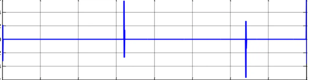
2.5 Detection in presence of noise
The presence of noise in power quality disturbances creates a new challenge for detection as it is difficult to detect the exact location of disturbance in a high noisy environment with a low SNR(signal to noise ratio).The Presence of noise also affects the classification accuracy as the feature vectors to be extracted for classification will also contain the noise contribution and the exact quantity of noise present is quite uncertain and hence de-noising of the disturbance is necessary before feature extraction and classification. In this work the white Gaussian noise is added to the pure power quality disturbances as shown in Figure 2.4, Figure 2.5 and Figure 2.6 to simulate a low SNR of 5 dB.The white Gaussian noise added to different PQ disturbances is shown in Figure 2.15.
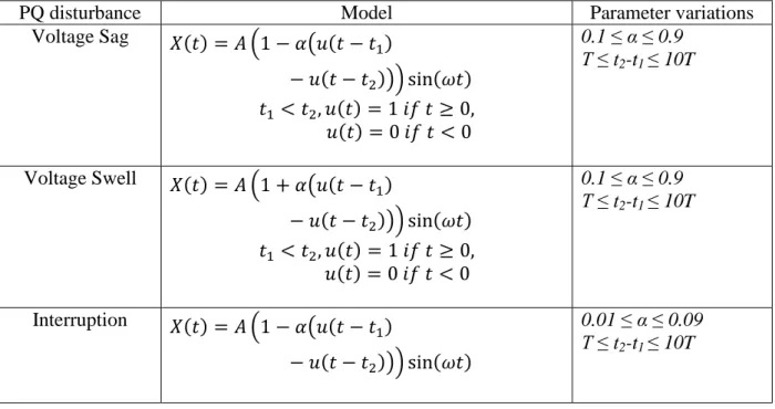
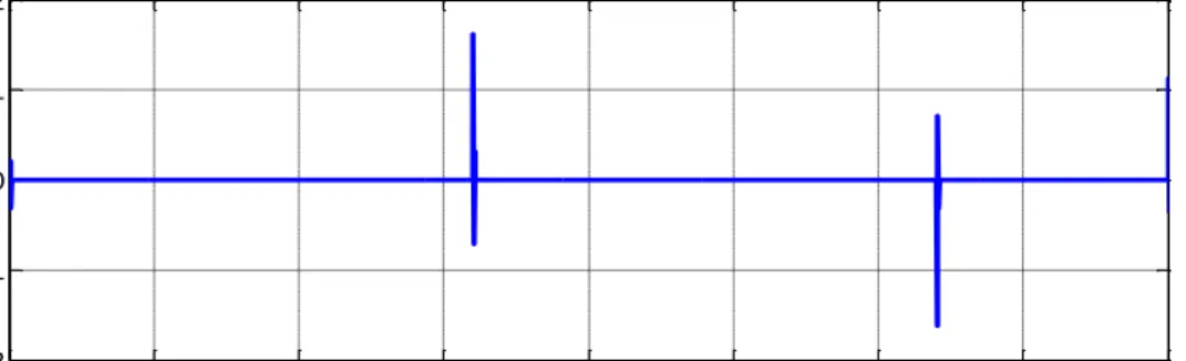
Figure 2.15 Additive white Gaussian noise
Figure 2.16 Sag polluted with noise
0 500 1000 1500 2000 2500 3000 -1.5 -1 -0.5 0 0.5 1 1.5 Samples M agn itude 0 500 1000 1500 2000 2500 3000 -2 -1 0 1 2 3 Samples M agn itude
Page 29
Figure 2.17 Swell polluted with noise
Figure 2.18 Interruption with noise 2.5.1 Difficulty in Detection in presence of noise
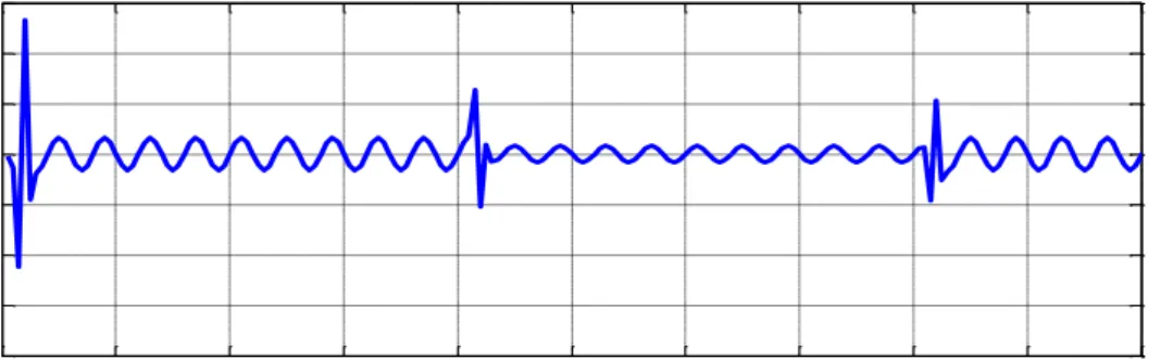
In the presence of noise, the localisation of disturbance is quite difficult which is shown below in Figure 2.19 in the case of Sag disturbance corrupted with noise. From the results obtained it is clearly observed that even after decomposing the disturbance into several levels the exact location of disturbance cannot be identified in terms of the detail coefficient of the disturbance which was easily identified in case of the disturbance without noise.
Figure 2.19 (a) Decomposed Sag with noise using WT
0 500 1000 1500 2000 2500 3000 -3 -2 -1 0 1 2 3 Samples M agn itude 0 500 1000 1500 2000 2500 3000 -2 -1 0 1 2 3 Samples M agn itude 0 500 1000 1500 2000 2500 3000 -3 -2 -1 0 1 2 3 Samples M agn itude
Page 30
Figure 2.19 (b) Approximate signal level 1
Figure 2.19 (c) Detail Signal Level 1
Figure 2.19 (d) Detail Signal Level 2
Figure 2.19 (e) Detail Signal Level 3
0 200 400 600 800 1000 1200 1400 1600 -3 -2 -1 0 1 2 3 Samples M agn itude 0 200 400 600 800 1000 1200 1400 1600 -1.5 -1 -0.5 0 0.5 1 Samples M agn itude 0 100 200 300 400 500 600 700 800 -1 -0.5 0 0.5 1 1.5 Samples M agn itude 0 50 100 150 200 250 300 350 400 -1.5 -1 -0.5 0 0.5 1 Samples M agn itude
Page 31
Figure 2.19 (f) Detail Signal Level 4
Figure 2.19 (g) Detail Signal Level 5
From the results shown in Figure 2.19 it is quite clear that in spite of decomposing the disturbance corrupted with noise into several levels accurate localisation of disturbing instant cannot be obtained in terms of detail coefficients as shown in Figure 2.19 (c),(d),(e),(f)and (g). These conditions are not ideal for the detection of the disturbances as well as for the feature extraction as it contains a high percentage of noise which may degrade the classification accuracy.
2.6 Summary
From the decomposition results obtained in this work it is quite evident that the Wavelet transform as a tool for detecting PQ disturbances works very well and can be employed effectively in designing a monitoring system for power quality events. Here different PQ disturbances like sag, swell, interruption, and some complex disturbances like sag with harmonics and swell with harmonics are decomposed into several levels and correctly located the point of disturbance. The problem occurs when the disturbances are corrupted with noise, accurate localisation of disturbing instant is difficult in terms of the detail coefficients. Hence in presence of noise direct decomposition of the disturbances with WT is not sufficient, so de-noising of disturbances is necessary before feature extraction and classification otherwise the classification accuracy is going to decrease as the feature vector to be extracted will
0 20 40 60 80 100 120 140 160 180 200 -1 -0.5 0 0.5 1 Samples M agn itude 0 10 20 30 40 50 60 70 80 90 100 -1.5 -1 -0.5 0 0.5 1 1.5 Samples M agn itude
Page 32
contain a high percentage of noise. Hence de-noising is very much necessary. A de-noising technique is discussed in the next chapter.
Page 33
3.1 Introduction
The proper detection i.e. the critical start-time and end-time of power quality (PQ) disturbances is an important aspect in monitoring and locating of the fault instances so as to extract the features and develop a classification system but the signal under investigation is often polluted by noises, rendering the extraction of features a difficult task, especially if the noises have high frequency spectrum which overlaps with the frequency of the disturbances. The performance of the classification system would be greatly degraded, due to the difficulty in distinguishing the noises and the disturbances and also the feature vector to be extracted will contain noise. Hence it is an important application of wavelet analysis in power system to de-noise power quality signals so as to detect and locate the disturbing points as the presence of noise in power quality events may degrade the classification accuracy.In this chapter a wavelet based de-noising technique is discussed based on soft thresholding so as to de-noise the PQ disturbances and improve the performance of classification system.
3.2 De-nosing using WT
3.2.1 Steps involved in De-noisingBasically there are 3 steps involved in de-noising process which is mentioned below. Decomposition: This step involves selecting a proper mother wavelet and choosing a level n up to which the signal S is decomposed using the selected mother wavelet. The mother wavelet selected in this work is “db4” as it gives good results in dealing with PQ disturbances. The level of decomposition n is selected as per the requirement and in this case it is chosen five.
Detail coefficients Thresholding: For each level from 1 to n, a threshold is selected and soft thresholding is applied to the detailed coefficients.
Reconstruction: Wavelet reconstruction is computed based on the original approximation coefficients of level n and the modified detail coefficients of levels from 1 to n.
3.2.2 Thresholding based De-noising
In the first stage, the polluted sinusoidal signal is decomposed by selected wavelet basic function “Db4” to certain level, here up to 5 levels. Coefficients at each level are compared within this level and absolute maximum coefficient will be stored to be the threshold value at this level. The maximum coefficient is selected as it represents the maximum noise characteristic. Any coefficients higher than this value are totally noise unrelated, and are thus only possibly associated with power quality disturbance. After computation, five detailed
Page 34
threshold values and one approximate threshold value will be stored for future signal de-noising. In the second stage, the power quality disturbance signals polluted by noises are recorded as before. The disturbance signal is decomposed by the same wavelet basic function to the same level to generate wavelet transform coefficients. All the coefficients at each level will be thresholded by the corresponding threshold value that is determined by the previous stage. All those threshold values represent the maximum noise characteristics. Any coefficients after the thresholding are the disturbance coefficients. Therefore after decomposition, the coefficients of the signal are greater than the coefficients of the noise, so we can find a suitable T as a threshold value. When the wavelet coefficient is smaller than the threshold, it is considered that the wavelet coefficient is mainly caused by the noise, so that the coefficient is set to 0,and then discarded; When the wavelet coefficient is larger than the threshold, it is considered that wavelet coefficient is mainly caused by the signal, so that the coefficient is remained or shrinks to zero according to a fixed value, and then the signal de-noised can be reconstructed through the new wavelet coefficients using wavelet transform. The method can be modelled as shown below in (3.1).
S(n) X(n).e(n) (3.1) Where n=0,1,2…k-1
S(n) =Noisy Signal
X(n)=Useful Power Quality disturbance without noise e(n)=The noise added to X(n)
3.2.3 Selection of Thresholding function
The thresholding on the DWT coefficients during wavelet based de-noising methods can be performed using either hard or soft Thresholding. The hard threshold method is ineffective, and Hard threshold function is not continuous, thus it is mathematically difficult to deal with, and also has some discontinuity points, while de-noising. The Soft threshold function is continuous, thus it is better to overcome the shortcomings of the Hard Thresholding but the soft threshold method transforms so smooth that transition of PQ signal is distorted and this method reduces the absolute value of the large wavelet factor, causing a certain amount of high-frequency loss of information and the result leads to edge blur of the signal. However the soft thresholding is best suited for de-noising of PQ disturbances.
Page 35 Soft Thresholding { | | | | Hard Thresholding { ( )( ) | | | |
Where Detail Coefficient at level n and scale j = Thresholding Value.
3.2.4 Selection of Thresholding rule
The selection of threshold value is crucial in wavelet based PQ signal de-noising. The careful rejection of the coefficients representing noise improves the accuracy of the de-noising results. Threshold is decisive to de-noising effect, and the common threshold selection rules present in MATLAB are: sqtwolog, rigrsure, heursure and minimaxi.
Rigrsure: 'rigrsure' uses for the soft threshold estimator, a threshold selection rule based on
Stein’s Unbiased Estimate of Risk (quadratic loss function). One gets an estimate of the risk for a particular threshold value (t). Minimizing the risks in (t) gives a selection of the threshold value.
Sqtwolog: 'sqtwolog' uses a fixed-form threshold yielding minimax performance multiplied
by a small factor proportional to log (length(X)).
Heursure: 'heursure' is a mixture of the two previous options. As a result, if the signal to
noise ratio is very small, the SURE estimate is very noisy. If such a situation is detected, the fixed form threshold is used.
Minimaxi: 'minimaxi' uses a fixed threshold chosen to yield minimax performance for mean
sqare error against an ideal procedure. The minimax principle is used in statistics in order to design estimators. Since the de-noised signal can be assimilated to the estimator of the
Page 36
unknown regression function, the minimax estimator is the one that realizes the minimum of the maximum mean square error obtained for the worst function in a given set.
All the above rules employed a common thresholding formula which is also known as automatic thresholding rule.
(√ ( )) (3.4) Where Threshold value at scale j
= Median value of Signal at scale j No of Coefficient at scale j
3.3 Results and discussion
The de-noising of Power Quality disturbances is performed using automatic Thresholding method as explained in 3.2.2 by selecting a threshold value for each level and Thresholding the detail coefficient and finally reconstructing the signal with modified detail coefficient and original approximate coefficient.
3.3.1 De-noising of sag disturbance
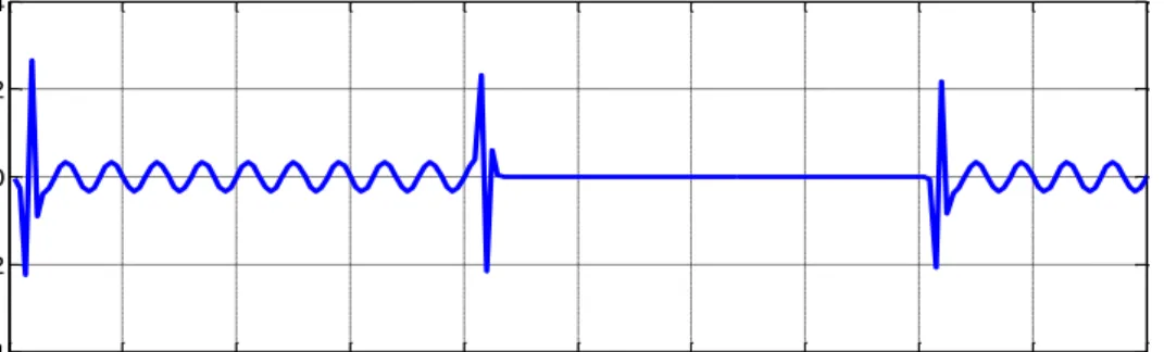
Figure 3.1 (a) De-noised sag disturbance
Figure 3.1 (b) Amount of noise cleared
0 500 1000 1500 2000 2500 3000 -1.5 -1 -0.5 0 0.5 1 1.5 Samples M agn itude 0 500 1000 1500 2000 2500 3000 -3 -2 -1 0 1 2 3 Samples M agn itude
Page 37
Figure 3.1 (c) Residue after de-noising
Figure 3.1 (a) is the noised Sag disturbance obtained after the implementation of the de-noising technique mentioned above in section 3.2.2. Figure 3.1(b) shows the amount of noise cleared which is obtained by subtracting the de-noised signal shown in Figure 3.1(a) from the noisy disturbance shown in Figure 2.16 in previous chapter.Figure 3.1(c) shows the residue after de-noising which is obtained by subtracting the de-noised signal obtained in Figure 3.1(a) from the Sag disturbance shown in Figure 2.4(b) in previous chapter.
3.3.2 De-noising of swell disturbance
Figure 3.2 (a) De-noised swell disturbance
Figure 3.2 (b) Amount of noise cleared
0 500 1000 1500 2000 2500 3000 -0.4 -0.2 0 0.2 0.4 Samples M agn itude 0 500 1000 1500 2000 2500 3000 -2 -1 0 1 2 Samples M agn itude 0 500 1000 1500 2000 2500 3000 -4 -2 0 2 4 Samples M agn itude
Page 38
Figure 3.2 (c) Residue after de-noising
Figure 3.2 (a) is the noised Sag disturbance obtained after the implementation of the de-noising technique mentioned above in section 3.2.2. Figure 3.2(b) shows the amount of noise cleared which is obtained by subtracting the de-noised signal shown in Figure 3.2(a) from the noisy disturbance shown in Figure 2.17 in previous chapter.Figure 3.2(c) shows the residue after de-noising which is obtained by subtracting the de-noised signal obtained in Figure 3.2(a) from the Swell disturbance shown in Figure 2.5(b) in previous chapter.
3.3.3 De-noising of interruption disturbance
Figure 3.3 (a) De-noised interruption disturbance
Figure 3.3 (b) Amount of noise cleared
0 500 1000 1500 2000 2500 3000 -0.6 -0.4 -0.2 0 0.2 0.4 Samples M agn itude 0 500 1000 1500 2000 2500 3000 -1.5 -1 -0.5 0 0.5 1 1.5 Samples M agn itude 0 500 1000 1500 2000 2500 3000 -3 -2 -1 0 1 2 3 Samples M agn itude
Page 39
Figure 3.3 (c) Residue after de-noising
Figure 3.3 (a) is the noised Sag disturbance obtained after the implementation of the de-noising technique mentioned above in section 3.2.2. Figure 3.3(b) shows the amount of noise cleared which is obtained by subtracting the de-noised signal shown in Figure 3.3(a) from the noisy disturbance shown in Figure 2.18 in previous chapter.Figure 3.3(c) shows the residue after de-noising which is obtained by subtracting the de-noised signal obtained in Figure 3.3(a) from the Swell disturbance shown in Figure 2.6(b) in previous chapter.
3.4 Performance indices
The Effectiveness of a denoising technique can be measured or quantified based on certain performance parameters such as MSE(mean square error) and SNR(signal to noise ratio).If the MSE is lower and SNR is higher after the noising it represents a good de-noising technique.
Mean Square Error: Effectiveness of a de-noising scheme is also evaluated by mean square error (MSE) defined as
N ii
D
i
V
N MSE 1 2))
(
)
(
(
1 (3.5)Where D(i) =De-noised Signal obtained
V(i) =Reference Power Quality Signal without Noise N=Length of the Signal
Signal to Noise Ratio: The signal to noise ratio (SNR) is defined as
N i N ii
D
i
V
V
i dB SNR 1 2 1 2 10))
(
)
(
(
log
) ( 10 ) ( (3.6) 0 500 1000 1500 2000 2500 3000 -0.4 -0.2 0 0.2 0.4 Samples M agn itudePage 40
An effective de-noising method requires low mean square error (MSE) and high SNR.Table3.1 shows the performance indices for Sag, Swell and Interruption disturbance.
Table3.1 Performance Indices
Type of Disturbance MSE SNR after De-noising(dB)
Sag 0.0033 20.3171
Swell 0.0292 14.0962
Interruption 0.0097 14.9200
3.5 Summary
The results obtained in this chapter shows that the wavelet transform can be used effectively to de-noise different power quality disturbances. In this chapter a thresholding based de-noising technique is discussed which is quite efficient in de-noise different PQ events. The efficiency of the de-noising is evident from the performance parameters. A system can never be completely noise free as it is an ideal case. But with the help of the technique discussed above adequate amount of noise can be cleared which ensures very less percentage of noise in feature vector and hence improves the classification accuracy.
Page 41
4.1 Introduction
The feature extraction is an important task in designing a monitoring system which will indicate the type of PQ disturbance occurring in the power system. A database is needed to be prepared based on some distinct parameters which will help in distinguishing different PQ disturbances with least amount of ambiguity. In this work after de-noising of PQ events, total harmonic distortion (THD) and Energy of the signal are used as the two distinctive parameters for feature extraction and preparing of the database. These databases are used as input to the fuzzy expert system for the classification purpose and also these databases are required to train the neural network so that a power quality disturbance (PQD) detection system can be modelled.
4.2 Feature vector
4.2.1 Total harmonic distortion
The distortion harmonics that included in each frequency ranges can be detected by using the approximation and the detailed coefficients which measure from sub band harmonics in terms of RMS value as (4.1)
n jn
cD
N
j RMS(
)
2 1 (4.1)Where Nj is the no of detail coefficients at scale j while THD is calculated by considering each sub-band contribution [11-12] as shown in equation (4.2).The sampling frequency selected is 6.4 kHz or 128f1. In this paper, the fundamental frequency is 50 hertz and used six
level of WT thus the output should receive the sub-band as follows: • cD1: 32f1 ~ 64f1; • cD2: 16 f1 ~ 32 f1; • cD3: 8 f1 ~ 16 f1; • cD4: 4 f1 ~ 8 f1; • cD5: 2 f1 ~ 4 f1; • cD6: 1 f1 ~ 2 f1; • cA6: 0 f1 ~ 1 f1;
Page 42