Int. J. Robust. Nonlinear Control2015;00:1–19
Published online in Wiley InterScience (www.interscience.wiley.com). DOI: 10.1002/rnc
Robust
H
∞Controller Design Using Frequency-Domain Data via
Convex Optimization
Alireza Karimi, Achille Nicoletti and Yuanming Zhu
Automatic Control Laboratory, Ecole Polytechnique F´ed´erale de Lausanne (EPFL), Lausanne, Switzerland
SUMMARY
A new robust controller design method that satisfies the H∞ criterion is developed for linear time-invariant single-input single-output (SISO) systems. A data-driven approach is implemented in order to avoid the unmodeled dynamics associated with parametric models. This data-driven method uses fixed order controllers to satisfy the H∞ criterion in the frequency domain. The necessary and sufficient conditions for the existence of such controllers are presented by a set of convex constraints. These conditions are also extended to systems with frequency-domain uncertainties in polytopic form. It is shown that the upper bound on the weighted infinity norm of the sensitivity function converges monotonically to the optimal value, when the controller order increases. Additionally, the practical issues involved in computing fixed-order rational H∞controllers in discrete- or continuous-time by convex optimization techniques are addressed. Copyright
c
2015 John Wiley & Sons, Ltd.
Received . . .
KEY WORDS: Data-driven control; robust control;H∞control
1. INTRODUCTION
Data-driven controller design is a very attractive research field within the control community (for a survey, see [1,2, 3]). In this method, a controller is designed by using either the time-domain or frequency-domain data of a system rather than by using a parametric model of the plant, where the intermediate identification procedure or first principle modeling is not required. Thus, they are expected to perform better than the model based approaches because of the absence of unmodelled dynamics and parametric errors (see [4]).
The majority of the data-driven methods use time-domain data for computing a controller that minimizes a model reference criterion (or more generally, anH2control criterion). Model Reference Adaptive Control (MRAC) [5], adaptive switching control [6,7], Iterative Feedback Tuning (IFT)
∗Correspondence to: Alireza Karimi:[email protected]
Contract/grant sponsor: The work of Yuanming Zhu is partially supported by Chinese Scholarship Council and the National Natural Science Foundation of China; contract/grant number: 61120106009
[8], Virtual Reference Feedback Tuning (VRFT) [9] and Iterative Correlation-based Tuning (ICbT) [10] are among the well-known methods using time-domain data.
There are only a few methods that use the frequency-domain data to compute robust controllers to meet some constraints on the stability margins or H∞ norm of the sensitivity functions. The frequency-domain methods assume that the frequency response of a system is available from an experiment (i.e., in applications where the parametric model is unknown or unavailable). These methods are closely related to time-domain data-driven methods because there is a linear relationship between the time-domain and frequency-domain data (through the Fourier transform). In this paper, the data-driven framework refers to a design method which uses the frequency response of a system in order to compute a robust controller.
A robust fixed-order controller design method using linear programming is proposed in [11]. In this method, the constraints on the gain margin, phase margin and crossover frequency are approximated with linear constraints by using linearly parameterized controllers. The frequency response data are used in [12] to compute the frequency response of a controller that achieves a desired closed-loop pole location. In [13], a complete set of PID controllers is computed that guarantee a gain margin, phase margin andH∞performance specification using frequency-domain data. This method is extended to design fixed-order linearly parameterized controllers in [14]. A data-driven synthesis methodology with a fixed structure controller that ensuresH∞performance is presented in [15]. This method, however, uses theQparameterization in the frequency domain and solves a non-convex optimization problem to find a local optimum. Another frequency-domain approach is presented in [16] to design reduced order controllers with a guaranteed bounded error on the difference between the desired and achieved magnitude of closed-loop sensitivity functions; this approach also uses a non-convex optimization method. A convex optimization method is used in [17] to compute robustH∞controllers for SISO systems represented by their frequency response. An interpretation of this algorithm based on convex-concave optimization for tuning PID controllers is given in [18]. This approach is extended to compute decoupling controllers for multi-input-multi-output (MIMO) systems in [19]. Based on this method, a public domain toolbox forMATLAB is developed which is available in [20].
In this paper, the necessary and sufficient conditions for the existence of robust controllers that guarantee bounded infinity norm on the sensitivity functions are developed. It is shown that these conditions depend only on the frequency response of the plant model and can be represented by convex constraints with respect to the controller parameters. By using fixed-order rational controllers, a convex optimization problem is formulated which produces a solution that ensuresH∞
performance. The results are extended to systems with frequency-domain polytopic uncertainties that are caused by measurement noise or multimodel incertitude. The developed conditions are necessary and sufficient for stable systems and only sufficient for unstable systems with polytopic uncertainties. The main contributions with respect to the work in [17] are: (1) The existence of a multiplier that convexifies the problem is proved (no linearization around a given desired open loop transfer function is performed). (2) Rational controllers are designed instead of linearly parameterized controllers. (3) The convergence of the method to the global optimal solution is proved.
This paper is organized as follows: the system structure and general preliminaries are discussed in Section2. The problem formulation and main results with regards to satisfying theH∞criterion
are addressed in Section 3. The implementation issues associated with the optimization problem are considered in Section4. The effectiveness of the proposed design scheme is demonstrated with simulation examples and experimental results in Section5. Finally, the concluding remarks are given in Section6.
2. PRELIMINARIES
LetRH∞represent the family of all stable, proper, real-rational transfer functions. It is imperative to note that RH∞ is closed under multiplication and addition (i.e., if A(s), B(s)∈RH∞, then
{A(s) +B(s), A(s)B(s)} ∈RH∞). Suppose that a SISO unity feedback control system structure is used where the plant is represented as G(s) =N(s)M−1(s)such that{N(s), M(s)} ∈RH∞. As asserted in [21] and [22], ifN(s)andM(s)are coprime, thenG(s) =N(s)M−1(s)is called a
coprime factorizationofG(s)overRH∞.
The frequency response of such a factorized SISO system is given by:
G(jω) =N(jω)M−1(jω), ω∈Ω (1) where Ω :=R∪ {∞} and N(jω), M(jω) are the frequency responses of bounded analytic functions in the right half plane. It is also assumed thatG(j∞) = 0, which implies thatN(j∞) = 0 andM(j∞)= 0. This representation includes time-delayed systems as well as unstable plants with unbounded infinity norms.
Finding the coprime factors of a given plant is a standard problem in control when the model of the plant is available ([23]). In a data-driven setting, for stable systems, a trivial choice is
N(jω) =G(jω)andM(jω) = 1. For unstable systems, a stabilizing controller is needed in order to properly formulateN(jω)andM(jω). In this case,N(jω) is the frequency response function between the reference signal and the measured output, while M(jω) is the frequency response function between the reference signal and the plant input. Given these definitions, it is evident that
N(jω)M−1(jω)represents the frequency response of the plant model. For notation purposes, the dependence onjωwill be omitted and will be reiterated when deemed necessary.
Consider the controller structure,K=XY−1, whereX andY are stable transfer functions with bounded infinity norm (X, Y ∈RH∞). These transfer functions may be discrete- or continuous-time; however, for presentation purposes, the continuous-time transfer functions will be considered. Note that the methods proposed in this work can also be used for computing discrete-time controllers. This will be shown through a simulation example in Section5.
The objective is to design a controller that meets some constraints on the infinity norm of the weighted sensitivity functions. Some of the sensitivity functions associated with the unity feedback control system structure are given by:
S = (1 +GK)−1=MY(NX+MY)−1 (2)
T = GK(1 +GK)−1=NX(NX+MY)−1 (3)
U = K(1 +GK)−1=MX(NX+MY)−1 (4)
An upper bound on the infinity-norm ofH(jω) =W1(jω)S(jω)will be considered, whereW1(jω) is the frequency function of a stable system with bounded infinity norm. Therefore, the control objective is to find a stabilizing controllerKsuch that
sup
ω∈Ω|H(jω)|< γ (6) This condition can easily be extended to the other weighted sensitivity functions asserted in equations (2-5).
3. CONVEX PARAMETERIZATION OF ROBUST CONTROLLERS
The main objective is to find a set of convex constraints (with respect toX andY) to satisfy the constraint in (6). The following lemma will be used in the proof of the main results of this paper:
Lemma 1
Suppose that H(jω) =W1MY(NX+MY)−1 is the frequency response of a bounded analytic function in the right half plane. Then, (6) is met if and only if there exists a stable proper rational transfer functionF(s)that satisfies
Re{(NX+MY −γ−1|W
1MY|)F(jω)}>0, ∀ω∈Ω
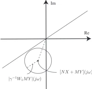
Proof : The basic idea is similar to that of the proof of Theorem 1 in [24]. From Fig.1, it is clear that (6) is satisfied if and only if the disk of radiusγ−1|W1MY|centered atNX+MY does not include the origin for all ω∈Ω, i.e. |NX+MY|> γ−1|W1MY|. This is equivalent to the existence of a line passing through origin that does not intersect the disk. Therefore, at every given frequency,ω, there exists a complex numberf(jω)that can rotate the disk such that it lays inside the right hand side of the imaginary axis. Hence, we have
Re{(NX+MY −γ−1|W
1MY|)f(jω)}>0 (7)
for allω∈Ω. In [24], it is shown that,f(jω)can be approximated arbitrarily well by the frequency response of a rational stable transfer functionF(s)if and only if
Z= (NX+MY −γ−1
0 |W1MY|)−1 (8)
is analytic in the right half plane for all γ0> γ. However, (NX+MY)−1 is stable because of the stability of H. On the other hand, by decreasingγ0 from infinity toγ, the poles of Z move continuously withγ0. Therefore,Zis not analytic in the right half plane if and only ifZ−1(jω) = 0 for a given frequency, which is not the case because the disk shown in Fig.1does not include the
[NX+MY](jω) |γ−1W
1MY|(jω)
Re Im
Figure 1. Graphical illustration of nominal performance
3.1. Nominal and robust performance
The set of all controllers that meet the nominal performance condition defined by the weighted norm of sensitivity functions is asserted in the following theorem.
Theorem 1
Given the frequency response modelGin (1) and the frequency response of a bounded weighting filterW1, the following statements are equivalent:
(a)There exists a controllerKthat stabilizesGand sup
ω∈Ω|W1(1 +GK)
−1|< γ (9)
(b)There existX, Y ∈RH∞withK=XY−1, such that
γ−1|W
1MY|(jω)< Re{[NX+MY](jω)}, ∀ω∈Ω (10)
Proof :(b⇒a) SinceNX+MY is analytic in the right half plane and its real part is positive for allω∈Ω, it will not encircle the origin whenωtravels along the Nyquist contour, so its inverse is stable and thereforeKstabilizesG. On the other hand, we have
|[NX+MY](jω)| ≥Re{[NX+MY](jω)}, ∀ω∈Ω which leads to
|W1MY|(jω)< γ|NX+MY|(jω) ∀ω∈Ω and consequently to (9) in Statement (a).
(a⇒b) Assume thatK=X0Y0−1satisfies Statement (a) but not Statement (b). Then, according to Lemma1there exists a stable proper rational transfer functionF(s), such that
Therefore, there exist X=X0F and Y =Y0F with K=XY−1=X0Y0−1, such that Statement
(b) holds.
The necessary and sufficient conditions for robust performance of closed-loop systems with disk-type frequency-domain uncertainty can be developed in a similar manner. Suppose that the frequency response of the plant model with some disk additive uncertainty is given as :
˜
N(jω) =N(jω) +|Wn(jω)|δnejθn ˜
M(jω) =M(jω) +|Wm(jω)|δmejθm
(11)
where|δn| ≤1,|δm| ≤1;θn, θm∈[0,2π];WnandWmare computed from the covariance of the estimates for a given confidence interval (see [25]). These types of models can be easily obtained by spectral analysis of measured data.
If we consider the nominal performance as defined in (6), the robust performance condition given by [22]: |W1MY˜ |< γ|MY˜ + ˜NX| ∀ω∈Ω (12) |W1M+W1|Wm|δmejθmY|< γ|MY˜ + ˜NX+|Wm|δmejθm+|Wn|δnejθn| ∀ω∈Ω (13) becomes: sup ω∈Ω |W1MY|+|W1WmY| |NX+MY| − |WnX| − |WmY| < γ (14)
Equivalently, at anyω∈Ω, a disk of radius
r(ω) =γ−1|W1MY|+γ−1|W1WmY|+|WnX|+|WmY| (15) centered at[NX+MY](jω)should not include the origin. This can be presented as a set of convex constraints with respect toX andY as follows:
r(ω)< Re{[NX+MY](jω)}, ∀ω∈Ω (16)
3.2. Multimodel and frequency-domain polytopic uncertainty
Let the frequency-domain polytopic uncertainty be defined as:
G(λ, jω) =N(λ, jω)M−1(λ, jω) (17) where N(λ, jω) = m i=1 λiNi(jω) ; M(λ, jω) = m i=1 λiMi(jω)
λi≥0,qi=1λi= 1andλis the convex hull ofλi’s. This uncertainty should not be confound with
the parametric polytopic uncertainty, which is defined in the parameter space in model-based robust control approaches.
It is clear that the following constraints
γ−1|W
are necessary and sufficient conditions for robust performance of the closed-loop system with multimodel uncertainty. However, it can be shown that there are only sufficient for frequency-domain polytopic uncertainty. It suffices to compute the convex combination of the constraints in (18) as γ−1m i=1 λi|W1MiY|< Re m i=1 λi[NiX+MiY] ,∀ω∈Ω and fori= 1, . . . , m. Noting that:
m i=1 λiW1MiY ≤ m i=1 λi|W1MiY| (19) we obtain: γ−1|W 1M(λ)Y|< Re{N(λ)X+M(λ)Y](jω)}, ∀ω∈Ω
Then, according to Theorem1, the upper bound for the weighted sensitivity function is satisfied for allλ.
Although the constraints for polytopic uncertainty are only sufficient, the necessary and sufficient conditions can be developed for some class of models and some sensitivity functions. The following theorem represents the results for systems that have polytopic uncertainty only inN.
Theorem 2
Consider the model given in (17) with N(λ, jω) =m
i=1λiNi(jω)and M(λ, jω) =M(jω). Then, the following statements are equivalent:
(a)ControllerKstabilizesG(λ) =N(λ)M−1and sup
ω∈Ω|W1(1 +G(λ)K)
−1|< γ (b)There existX, Y ∈RH∞such thatK=XY−1, and
γ−1|W
1MY(jω)|< Re{[NiX+MY](jω)}, ∀ω∈Ω, for i= 1, . . . , m (20)
Proof :(b⇒a) The convex combination of the constraints in (20) leads to
γ−1|W
1MY(jω)|< Re{[N(λ)X+MY](jω)} (21) for allω∈Ωand for allλ. So Statement (a) can be concluded using the result of Theorem1.
(a ⇒b) Suppose that (a) is satisfied with the controllerK=X0Y0−1. Therefore, all disks of the same radius,γ−1|W1MY0|, centered inside a polygon withm vertices,NiX0+MY0, do not include the origin. This represents a convex set, which is the convex hull of themdisks. Therefore, there exists a line that passes through the origin and does not intersect this convex set. As a result, similar to the proof of Lemma1, there exists a stable transfer functionF(s)such that:
Re{[NiX0+MY0−γ−1|W1MY0|]F(jω)}>0, ∀ω∈Ω, for i= 1, . . . , m
[N2X0+M2Y0](jω)
γ−1|W1M1Y0|(jω)
γ−1|W1M3Y0|(jω)
Re Im
Figure 2. Illustration of the constraints for polytopic uncertainty with 3 vertices
Remark: Theorem 2 considers only the plant model with polytopic uncertainty in N. This represents the class of stable systems that may have some fixed poles on the imaginary axis. The theorem also holds for unstable systems with no uncertainty inM. A polytopic uncertainty inM will change the radius of the disks centered atNiX0+MiY0, such that the whole set of the disks will not be necessarily convex. Figure2shows a case in which the set of the disks is not convex but is inside the convex hull of the disks. This is always true because of the constraint in (19). In the special case shown in Fig.2, we observe that the set of disks does not include the origin but the convex hull does. Similarly, Statement (b) in Theorem2is a sufficient condition for satisfying an upper bound on the weighted sensitivity functionsT orV, since the radius of the disks, at each frequency, will not be constant for the whole polygon. However, it will be necessary and sufficient for an upper bound on the weighted sensitivity functionU in (4).
3.3. Parametric uncertainty
The approach proposed in this paper requires only the frequency response of a model to design a robust controller. However, if a parametric model is available, the approach can be still used by computing the frequency response of the model. It is well known that the interval deterministic parametric uncertainty cannot be converted to the ellipsoid uncertainty in the frequency-domain. In a data-driven framework, for an identified parametric model using noisy data, the parametric uncertainties have stochastic bounds and can be transferred to the frequency-domain in a stochastic sense.
In a data-driven approach, a parametric model of the plant is identified together with its parametric uncertainty using the classical prediction error methods (see [25]). The parametric uncertainty is characterized by an ellipsoid in the parameter space and can be computed using the asymptotic covariance matrix of the parameters for a given probability level. Thanks to the invariance property
of the Maximum Likelihood Estimators, any function of the estimated parameters will converge to a normal distribution with a covariance matrix that can be computed based on the derivative of the function with respect to the parameters and its covariance matrix. In the complex plane, this parametric uncertainty is represented by an ellipse at each frequency that is well approximated with anm-side polygon (m >2) of minimum area that circumscribes each ellipse. In this manner, the parametric uncertainty can be taken into account using the frequency-domain polytopic uncertainty with almost no conservatism.
Suppose that a stable parametric model Gˆ(θ) is identified from a set of noisy data and the covariance matrix of the parameters, cov(θ), is computed. Then, the frequency response of the identified model can be computed and its real and imaginary parts put in a vector as:
ˆ
Gv(ω) =
Re{Gˆ(jω)} Im{Gˆ(jω)}T (22) This vector has a joint normal distribution with the covarianceCG(ω)that can be estimated from cov(θ)using a linear approximation as follows:
CG(ω) = ∂Gˆv(ω) ∂θ cov(θ) ∂Gˆv(ω) ∂θ T (23)
Note that θ∈Rn, cov(θ)∈Rn×n and CG(ω)∈R2×2. Then, the true frequency response will belong to the following ellipse in the complex plane with a probability of1−α:
x−Re{Gˆ} y−Im{Gˆ} T C−1 G (ω) x−Re{Gˆ} y−Im{Gˆ} ≤ X2 2(α) (24)
where X22 is the chi-square distribution with two degrees of freedom. For a confidence interval of 0.95 (α= 0.05), we have X22(0.05) = 5.99. Since the uncertainty set is an ellipse, the disk uncertainty in (11) cannot be used to model it without conservatism. However, the ellipse can be represented by annq-sided polygon with minimum area that circumscribes it, and is approximated by frequency-domain polytopic uncertainty as:
G(λ) = nq k=1 λiGˆk(jω) (25) where ˆ Gk(jω) = ˆG(jω) + [1 j]5.99CG(ω) cos(2πk/n w) cos(π/nq) sin(2πk/nw) cos(π/nq) (26) The last vector in (26) represents thek-th coordinate of a vertex of a polygon circumscribing the unit circle while the matrix5.99CG(ω)designates the size and direction of the uncertainty (for 0.95 probability).
4. FIXED-ORDER CONTROLLER DESIGN
The minimization of theH∞norm becomes an optimization problem that can be solved as follows: min
X,Y γ
subject to
|W1MY(jω)|< γRe{[NX+MY](jω)},∀ω∈Ω
(27)
In general, this optimization problem is not convex. However, by linearly parameterizing the controllersX andY, it becomes a quasi-convex optimization problem and can be solved by using a bisection algorithm to obtain the optimal solution for γ. Within a given tolerance, the bisection algorithm ensures the convergence to the global optimum solution. There are several practical and implementation issues in this optimization problem that will be addressed in this section.
4.1. Controller parameterization
A linear parameterization ofX andY keeps the constraints in (27) convex. As a result,X(s)and
Y(s)are linearly parameterized asX(s) =ρTxφ(s)andY(s) =ρTyφ(s), whereρTx = [ρx0, . . . , ρxn] andρTy = [1, ρy1, . . . , ρyn]are the vectors of the controller parameters and
φT(s) = [1, φ
1(s)· · ·, φn(s)] (28)
is a vector of stable orthogonal basis functions. A simple choice is the Laguerre basis functions given by
φi(s) = √
2ξ(s−ξ)i−1 (s+ξ)i
withξ >0andi= 1,· · ·, n. These basis functions have only one parameter to be selected (ξ). The effect of the Laguerre parameter on the control performance for low order controllers is illustrated in a simulation example in the next section.
4.2. Convergence to the optimal solution
In this sub-section, we will show that the optimal solution (γn) to the optimization problem in (27) (for a linear parameterization ofXandY by the orthogonal basis functions of ordern) will converge to the least upper bound of the infinity norm of the weighted sensitivity function whenngoes to infinity. The following Lemma is required to prove this convergence:
Lemma 2
([26]) LetXn∗(s)be the projection ofXo(s)∈RH∞into the subspace spanned by the orthogonal basis functionsφ(s)in (28). Then
lim
n→∞Xo−X ∗ n∞= 0
Theorem 3
Suppose that the controller Ko(s) achieves the optimal H∞ performance for the plant model
G=NM−1such that
γo= inf
K supω |W1(1 +GK)|= supω |W1(1 +GKo)|
Suppose also that γn is the optimal solution of the convex optimization problem in (27) when
X and Y are parameterized by an n dimensional orthogonal basis function. Thenγn converges monotonically from above toγowhenn→ ∞.
Proof : According to Theorem 1, there exist Xo(s), Yo(s)∈RH∞ such that Ko(s) =
Xo(s)Yo−1(s)and γo= sup ω∈Ω W1MYo NXo+MYo (29)
Take Xn∗ andYn∗ as the projections ofXo andYo into the subspace spanned by anndimensional orthogonal basis functions and define
γ∗ n= sup ω∈Ω W1MYn∗ NX∗ n+MYn∗ (30)
We assume thatγn∗ is bounded, i.e.,NXn∗+MYn∗has no zero on the imaginary axis. This can be proved ifnis large enough using contradiction and based on the fact thatNXo+MYo∞> >0. Assume thatjω∗is a zero ofNXn∗+MYn∗. Therefore, atω=ω∗, one has:
|NXo+MYo|=|N(Xo−Xn∗) +M(Yo−Yn∗)|> (31)
However, |N(Xo−Xn∗) +M(Yo−Yn∗)| can be made arbitrarily small by increasing n, which
shows that for large but finiten,NXn∗+MYn∗will not have a zero on the imaginary axis. Now, let us compute
|γ∗ n−γo| ≤sup ω∈Ω W1MYn∗ NX∗ n+MYn∗ − W1MYo NXo+MYo (32) ≤sup ω∈Ω W1MN[Xn∗(Yo−Yn∗)−Yn∗(Xo−Xn∗)] (NX∗ n+MYn∗)(NXo+MYo)
Moreover, according to Lemma2: lim
n→∞Xo−X ∗
n∞= 0, n→∞lim Yo−Yn∗∞= 0
Therefore, since all frequency functions in (32) are bounded and the denominator has no zero on the imaginary axis
lim n→∞|γ
∗
n−γo|= 0 (33)
On the other hand,γn is always less than or equal toγn∗ and greater than the optimal solutionγo. Thusγnconverges from above toγoand this convergence is monotonic because the basis functions
4.3. Finite number of constraints
The constraints in (27) should be satisfied for all ω∈Ω, which is an infinite set. This problem is known as semi-infinite programming (SIP) problem and there exist different methods to solve it. A very simple and practical solution to this problem is to choose a finite set of frequencies Ωp={ω1, ω2,· · ·, ωp} and satisfy the constraints for this set. In this manner, the optimization
problem is converted to a semi-definite programming (SDP) problem which can be solved efficiently with solvers that are readily available.
Another solution is to use a randomized approach where the constraints are satisfied for a finite set of randomly chosen frequencies. In this approach, a bound on the violation probability of the constraints can be derived and approaches zero when the number of samples goes to infinity (see [27] and [28]). It should be mentioned that in a data-driven framework, the frequency domain uncertainties are given by some stochastic bounds. Therefore, even if the constraints are met for all
ω, the stability, robustness and performance are guaranteed within a probability level. As a result, the use of randomized methods to solve the robust optimization problem in (27) is fully compatible with the uncertainty description of the frequency-domain model of the proposed approach.
4.4. Solution by linear programming
The convex constraints in (27) are equivalent to the following linear constraints:
Re{[NX+MY](jω)−γ−1ejθW
1MY(jω)}>0, (34)
∀ω∈Ωand∀θ∈[0,2π[. In fact,γ−1ejθW1MY(jω)represents the circle in Fig.1. Note thatejθ can be very well approximated by a polygon ofq >2vertices with least area that circumscribes it. By griddingωand bounding the circleejθ, a finite set of linear constraints can be obtained as:
Re [NX+MY](jωi)−γ−1 e j2πk/q cos(π/q)W1MY(jωi) >0 (35) fori= 1, . . . , pandk= 1, . . . , q. Therefore, the convex constraints in (27) can be replaced byp×q linear constraints.
5. CASE STUDIES
5.1. Case 1: Multimodel uncertainty
In this example, a simulation is carried out to compare the traditionalµ-synthesis method and the proposed approach for a set of unstable models. The controlled plants are taken from an example in the robust control toolbox ofMATLAB. The nominal plant model is a first-order unstable system
G0(s) = 2(s−2)−1, and the family of perturbed plants are variations ofG0(s)as follows, G1(s) =G0(s)·(0.06s+ 1)−1 G2(s) =G0(s)·e−0.04s G3(s) =G0(s)·502(s2+ 10s+ 502)−1 G5(s) = 2.4(s−2.2)−1 G4(s) =G0(s)·702(s2+ 28s+ 702)−1 G6(s) = 1.6(s−1.8)−1
Remark: It is imperative to note that these models are simply used to obtain the frequency response functions of the perturbed plants. The actual controller synthesis does not rely on these parametric models.
Compared with the nominal plant,G1has an extra lag,G2has an additional time delay,G3and
G4 have high frequency resonance mode,G5 andG6have pole and gain migrations. The control task is to design a linear controller to simultaneously stabilize this family of unstable plants and minimize the infinity norm of the weighted sensitivity functions, i.e.:
minγ W1Si∞< γ , W2Ti∞< γ , for i= 0, . . . ,6 where W1(s) = 0s.33+ 0s.+ 4008496.248 ; W2(s) = 0.1975s 2+ 0.6284s+ 1 7.901e−5s2+ 0.2514s+ 400
Theµ-synthesis method from theMATLABrobust control toolbox is used to solve this problem. The multimodel uncertainty is approximated with a fourth-order uncertainty weighting filter and a 18th-order controller is designed that achieves a performance ofγo= 1.0248. Comparable performance is achieved after reducing the controller order to 6.
Continuous-time Laguerre basis functions of order 5 withξ= 20and an integrator are used for the controller parameterization. A high frequency pole at 100 is used for constructingNi andMi for the models. For example, forG6(s) =N6(s)M6−1(s):
N6(s) = s+ 1001.6 , M6(s) =ss+ 100−1.8
The frequency response of the model is computed at N = 200logarithmically spaced frequency points between10−3and104 rad/s. The linearized constraints in (35) are used with a polygon of
q= 25vertices for over bounding ejθ. Solving the optimization problem leads to the following controller:
K(s) =0.26773(s(ss+ 7+ 1)(.759)(s+ 2348)(s2+ 27s.772+ 19s+ 556.82s.5)(+ 131s2+ 94.3)(s.52s+ 28+ 12440).5s+ 3510)
which leads to the step disturbance response depicted in Fig.3. The resulting performance obtained from the proposed optimization problem isγo= 0.8852. This is much smaller than that of theµ -synthesis method; in the proposed approach, there is no conservatism in modeling the multimodel uncertainties. It should be mentioned that in theµ-synthesis approach the time delay in G2(s)is
0 0.5 1 1.5 2 −0.5 0 0.5 1 Time (seconds) Amplitude
Figure 3. Step responses of the family of closed-loop systems
approximated with a first-order Pade function, while the time-delay is taken into account with no approximation in the proposed approach.
5.2. Case 2: Convergence to optimal performance
Consider a discrete-time SISO system as follows:
G(z) =z3−1.116zz2−+ 00.186.465z−0.093, (36) The goal is to design a controller with an integrator that minimizesW1S∞, where
W1(z) = 0.4902(z
2−1.0431z+ 0.3263)
(z−1)(z−0.282) . (37)
For discrete-time controller synthesis, the controller is parameterized by discrete-time Laguerre basis functions as follows:
K(z) =X(z)Y−1(z) ; X(z) =ρT
xφ(z), Y(z) =ρTyφ(z)
wherenis the controller order,φT(z) = [1, φ1(z), . . . , φn(z)]with
φi(z) = √ 1−a2 z−a 1−az z−a i−1
and −1< a <1. It will be shown that by increasing the controller order, the side effect of the selection of the parameter of Laguerre function,a, is reduced.
2 3 4 5 6 7 8 9 10 0.55 0.56 0.57 0.58 0.59 0.6 0.61 0.62 0.63 Controller order γ n a=0 a=0.1 a=0.2 a=0.3 a=0.4 a=0.5
Figure 4.γnversus the controller order with different Laguerre parameter
In this example, 50 equally spaced frequency points between 0 and π are chosen. In order to have an integrator in the controller and to avoid unboundedness ofW1atω= 0, the basis functions forY(z)are multiplied by(z−1)/z. Since the system is stable, we chooseN(jω) =G(jω)and
M(jω) = 1. The convex constraints are linearized by approximatingejθwith a polygon ofq= 50 vertices.
The standardH∞control method in the Robust Control toolbox ofMATLABleads to the optimal value of γo= 0.552with a 6th order controller. Fig.4shows the optimal value,γn, for different choice of the parameter a in Laguerre basis function and different controller ordern. It can be observed that the optimal solution converges monotonically and is independent of the value ofa. The best results are obtained fora= 0, which almost achievesγofor an 8th-order controller.
5.3. Case 3: Flexible Transmission System
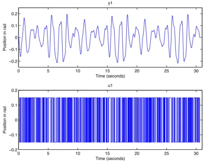
In this example, the experimental data are used to compute a robust controller with respect to frequency-domain uncertainty. An electro-mechanical flexible transmission system which consists of three disks connected by elastic belts is considered. The first disk is coupled to a servo motor which is derived by a current amplifier. The position of the third disk is measured with an incremental encoder and controlled by a proportional controller. The input of the system is the reference position for the third disk (see Fig.5). This system is excited by a PRBS signal with a sampling period of Ts= 40ms and the data length is 765. Figure6shows the experimental data that are used to identify a frequency domain model usingspacommand in Identification toolbox ofMATLAB. The Nyquist diagram of this spectral model together with the uncertainty disks of 0.95 probability are given in Fig.7. The uncertainty disks are approximated by a polygon ofm= 20 vertices and the goal is to design a stabilizing controller that minimizes γ whereW1S∞< γ,
drive disk load disk
speed reduction disk
Figure 5. Flexible transmission system
0 5 10 15 20 25 30 −0.2 −0.1 0 0.1 0.2 Time (seconds) Position in rad y1 0 5 10 15 20 25 30 −0.2 −0.1 0 0.1 0.2 u1 Time (seconds) Position in rad
Figure 6. Experimental identification data.
with
W1(z) =zz−−0.196
In the proposed method, discrete-time Laguerre basis functions of order 4 witha= 0(FIR filter) are considered forX andY. The resulting controller is
K(z) =20.3(z2−1.88z+ 0.92)(z2−1.278z+ 0.6057) (z+ 0.72)(z−1)(z2+ 0.209z+ 0.563) ,
which achieves an optimal performance of γ= 2.12. Figure8shows the magnitude of the Bode diagram of the sensitivity function for the nominal model. It can be observed that the sensitivity
−3 −2 −1 0 1 2 3 −5 −4 −3 −2 −1 0 Real axis imaginary axis
Figure 7. Nyquist diagram of the spectral model together with uncertainty disks
10−1 100 101 −30 −25 −20 −15 −10 −5 0 5 10
From: y1 To: Out(1)
Magnitude (dB)
Bode Diagram
Frequency (rad/s)
Figure 8. Magnitude Bode diagram of the sensitivity function
function is small at low frequencies and its maximum value is less than 5db which guarantees a good stability margin.
6. CONCLUSION
A robust controller design method for LTI-SISO systems based on frequency-domain data is proposed. In comparison with the classical H∞ controller design methods, the following features can be highlighted:
• The frequency response of the plant is the only requisite for controller synthesis where no parametric model is required
• Pure input/output time delay is considered with no approximation.
• Frequency-domain uncertainty is taken into account with reduced conservatism.
• Parametric uncertainty in identified models with noisy data can be considered in a stochastic sense with reduced conservatism.
• Fixed-order controllers can be designed in a convex optimization problem that considers a finite amount of constraints in the frequency domain.
It is shown that the choice of the basis functions affects the optimization results for low-order controllers. The optimal choice of the basis function and the extension to multivariable systems are considered for future research works.
REFERENCES
1. Bazanella AS, Campestrini L, Eckhard D.Data-driven Controller Design: TheH2Approach. Springer, 2012. 2. Hou ZS, Wang Z. From model-based control to data-driven control: Survey, classification and perspective.
Information Sciences2013;235:3–35.
3. Yin S, Li X, Gao H, Kaynak O. Data-based techniques focused on modern industry: an overview. Industrial Electronics, IEEE Transactions on2015;62(1):657–667.
4. Formentin S, van Heusden K, Karimi A. A comparison of model-based and data-driven controller tuning.
International Journal of Adaptive Control and Signal Processing2014;28(10):882–897.
5. Landau ID, Lozano R, M’Saad M, Karimi A.Adaptive Control: Algorithms, Analysis and Applications. Springer-Verlag: London, 2011.
6. Stefanovic M, Safonov MG.Safe adaptive control: Data-driven stability analysis and robust synthesis, vol. 405. Springer, 2011.
7. Battistelli G, Hespanha JP, Mosca E, Tesi P. Model-free adaptive switching control of time-varying plants.
Automatic Control, IEEE Transactions on2013;58(5):1208–1220.
8. Hjalmarsson H, Gevers M, Gunnarsson S, Lequin O. Iterative feedback tuning: Theory and application.IEEE Control Systems Magazine1998; :26–41.
9. Campi MC, Lecchini A, Savaresi SM. Virtual reference feedback tuning: A direct method for the design of feedback controllers.Automatica2002;38:1337–1346.
10. Karimi A, Miˇskovi´c L, Bonvin D. Iterative correlation-based controller tuning.Int. Journal of Adaptive Control and Signal Processing2004;18(8):645–664.
11. Karimi A, Kunze M, Longchamp R. Robust controller design by linear programming with application to a double-axis positioning system.Control Engineering PracticeFebruary 2007;15(2):197–208.
12. Hoogendijk R, Den Hamer AJ, Angelis G, van de Molengraft R, Steinbuch M. Frequency response data based optimal control using the data based symmetric root locus. IEEE Int. Conference on Control Applications, Yokohama, Japan, 2010; 257–262.
13. Keel LH, Bhattacharyya SP. Controller synthesis free of analytical models: Three term controllers.IEEE Trans. on Automatic ControlJuly 2008;53(6):1353–1369.
14. Parastvand H, Khosrowjerdi MJ. Controller synthesis free of analytical model: fixed-order controllers.Int. Journal of Systems Science2014; (ahead-of-print).
15. Den Hamer AJ, Weiland S, Steinbuch M. Model-free norm-based fixed structure controller synthesis.48th IEEE Conference on Decision and Control, Shanghai, China, 2009; 4030–4035.
16. Khadraoui S, Nounou H, Nounou M, Datta A, Bhattacharyya S. A measurement-based approach for designing reduced-order controllers with guaranteed bounded error.Int. Journal of Control2013;86(9):1586–1596. 17. Karimi A, Galdos G. Fixed-order H∞ controller design for nonparametric models by convex optimization.
Automatica2010;46(8):1388–1394.
18. Hast M, Astr¨om K, Bernhardsson B, Boyd S. Pid design by convex-concave optimization.Proceedings European Control Conference, Citeseer, 2013; 4460–4465.
19. Galdos G, Karimi A, Longchamp R.H∞controller design for spectral MIMO models by convex optimization.
Journal of Process Control2010;20(10):1175 – 1182.
20. Karimi A. Frequency-domain robust control toolbox.52nd IEEE Conference in Decision and Control, 2013; 3744 – 3749.
21. Zhou K, Doyle JC.Essentials of robust control. Prentice-Hall: N.Y., 1998.
22. Doyle CJ, Francis BA, Tannenbaum AR.Feedback Control Theory. Mc Millan: New York, 1992. 23. Zhou K.Essentials of Robust Control. Prentice Hall: New Jersey, 1998.
24. Rantzer A, Megretski A. Convex parameterization of robustly stabilizing controllers.IEEE Trans. on Automatic ControlSeptember 1994;39(9):1802–1808.
25. Ljung L.System Identification - Theory for the User. second edn., Prentice Hall: NJ, USA, 1999.
26. Akcay H, Ninness B. Orthonormal basis functions for continuous-time systems andlpconvergence.Mathematics of Control, Signals, and Systems1999;12:295–305.
27. Calafiore G, Campi MC. The scenario approach to robust control design.IEEE Trans. on Automatic ControlMay 2006;51(5):742–753.
28. Alamo T, Tempo R, Luque A. On the sample complexity of probabilistic analysis and design methods.Perspectives in Mathematical System Theory, Control, and Signal Processing. Springer, 2010; 39–55.