Distributed Optimal Control of Cyber Physical Systems: Controller Synthesis, Architecture Design and System Identification

(1)

Systems: Controller Synthesis, Architecture Design

and System Identification

Thesis by

Nikolai Matni

In Partial Fulfillment of the Requirements for the Degree of

Doctor of Philosophy

California Institute of Technology Pasadena, California

2016

(2)

(3)

(4)

Acknowledgments

I want to thank my advisor, John Doyle, for his generous support & encouragement during these years. He has been an incredible mentor and role model, constantly challenging me to grow as a researcher and providing me with opportunities rarely given to graduate students. He has changed the way that I view science, engineering and research, and for this I am eternally grateful. I also want to thank my unofficial co-advisor, Venkat Chandrasekaran. Venkat brings a rare elegance and sophistication to his work, and I am incredibly fortunate to have been able to collaborate with and learn from him these past few years.

I would also like to express my thanks to the remaining members of my thesis committee, Adam Wierman and Richard M. Murray, as well as to Steven Low, Joel Tropp, Babak Hassibi, Anders Rantzer and Joel Burdick. Be it through teaching, informal discussions, or collaborations, all of these amazing professors have played an instrumental role in making my time at Caltech intellectually stimulating and enjoyable. I would also like to thank Andrew Lamperski for his mentorship early in my graduate student career: without his guidance and support, this thesis would most certainly look very different. I must also thank my master’s advisor, Meeko Oishi, for introducing me to the field of control theory, and for giving me my first shot at research.

(5)

survived my time here without you.

(6)

List of Figures

1.1 A schematic diagram of norm-optimal control. The objective is to de-sign a feedback controller that minimizes the size (as measured by an appropriate signal-to-signal norm) of the system’s closed-loop response to the environment. . . 1 1.2 Schematics of centralized, decentralized and distributed control

archi-tectures. . . 3 1.3 A schematic of Witsenhausen’s counterexample [courtesy of wikipedia], a

control problem subject to non-classical information sharing constraints for which nonlinear control can arbitrarily outperform linear control. . 4 2.1 The graph depicts the communication structure of the three-player chain problem.

Edge weights (not shown) indicate the delay required to transmit information be-tween nodes. . . 13 3.1 The distributed plant considered in (3.6), shown here forD= 4. Dummy

(11)

3.2 The information graph _G = (_V,_E), and label sets _{Ls_t_}s∈V, for system (3.6), shown here for D = 4, and et = (3,2). Notice that: (i) for

each (r, s) _{∈ E}, with _|r_| < D + 1, we have that _|s_| = _|r_|+ 1, (ii) that _|s_|corresponds exactly to how delayed the information in the label set is, and (iii) that _LV_t contains all of the information at nodes s.t. |s_| > ei_t, s₃i. We also see that the graph is naturally divided into two branches, with each branch corresponding to information pertaining to a specific plant. . . 37 4.1 A diagram of the generalized plant defined in (4.2). . . 60 4.2 Examples of QI sparsity patterns generated via a) actuator, b) sensor,

and c) actuator/sensor RFD procedures without any distributed con-straints, and d) actuator RFD subject to nested information constraints. 66 4.3 Three player chain system . . . 73 4.4 Topology of system considered for RFD example. Solid lines indicate

both physical interconnections and existing communication links be-tween controllers. Dashed lines correspond to possible additional edges to be added. . . 79 4.5 A small degradation in closed loop performance allows for a significant

decrease in architectural complexity. . . 81 4.6 Resulting architecture for λ = 500: despite only using eight

(12)

5.3 The closed loop norms achieved by distributed optimal controllers imple-mented on communication graphs constructed by adding k = 1, . . . ,_|E_|

links to the base QI communication graph Γ6-chain are plotted as circles. The solid line denotes the performance achieved by distributed opti-mal controllers implemented on the communication graphs identified by the co-design procedure described in Algorithm 1. The dotted/dashed lines indicate the closed loop norm achieved by the distributed optimal controllers implemented on the base and maximal QI communication graphs, respectively. . . 129 5.4 The solid line denotes the performance achieved by distributed optimal

controllers implemented on the communication graphs identified by the co-design procedure described in Algorithm 1. The dotted and dashed lines indicate the closed loop norm achieved by the distributed optimal controllers implemented on the base and maximal QI communication graphs, respectively. . . 131 6.1 Illustrated in Figures 6.1 (a) and (b) are the full and hidden

interconnec-tion measurement cases, respectively. Dashed green lines correspond to low-order signals, and dotted/solid black/red lines correspond to mea-sured/hidden high-order interconnection signals. In the full measure-ment case, the high order dynamics of the large scale system are iso-lated from the local measurements, as the interconnection signals can simply be treated as inputs to the system. In the hidden interconnec-tion measurement setting, high order global signals “leak” into our local measurements via the hidden interconnection signal (solid red), but do so through a low-rank transfer function. . . 136 6.2 The graph depicts the physical interconnection structure of the

(13)

6.3 By examining how the values of the singular values of_H( ˆSi)vary across different values ofδ and δh, the order of the local subsystem is correctly

(14)

List of Tables

4.1 A dictionary relating various SLIP methods in structured inference and Actuator RFD problems. . . 76 4.2 Interpretation of parameters in Structured Controller Design and

Struc-tured Inference. . . 82 4.3 Summary of relevant values for the controllerU2 with actuators at nodes

(15)

Abstract

The centralized paradigm of a single controller and a single plant upon which modern control theory is built is no longer applicable to modern cyber-physical systems of interest, such as the power-grid, software defined networks or automated highways systems, as these are all large-scale and spatially distributed. Both the scale and the distributed nature of these systems has motivated the decentralization of control schemes into local sub-controllers that measure, exchange and act on locally available subsets of the globally available system information. This decentralization of con-trol logic leads to different decision makers acting on asymmetric information sets, introduces the need for coordination between them, and perhaps not surprisingly makes the resulting optimal control problem much harder to solve. In fact, shortly after such questions were posed, it was realized that seemingly simple decentralized optimal control problems are computationally intractable to solve, with the Wisten-hausen counterexample being a famous instance of this phenomenon. Spurred on by this perhaps discouraging result, a concerted 40 year effort to identify tractable classes of distributed optimal control problems culminated in the notion of quadratic invariance, which loosely states that if sub-controllers can exchange information with each other at least as quickly as the effect of their control actions propagates through the plant, then the resulting distributed optimal control problem admits a convex formulation.

(16)

with a particular focus on closing the gap between theory and practice by relaxing or removing assumptions made in the traditional distributed optimal control framework. Our contributions are to the foundational theory of distributed optimal control, and fall under three broad categories, namely controller synthesis, architecture design and system identification.

(17)

(18)

Chapter 1

ControllerkClosed Loop Systemk

Figure 1.1: A schematic diagram of norm-optimal control. The ob-jective is to design a feedback controller that minimizes the size (as measured by an appropriate signal-to-signal norm) of the sys-tem’s closed-loop response to the environment.

Robust and optimal control theory [2, 3] have been active areas of research since the 1970s: they aim to provide rigorous mathematical meth-ods for analyzing and designing complex cyber-physical systems that are composed of a cyber-physical plant coupled in feedback with a controller. The need for control theory, and robust control theory in particular, arises from the inherent uncertainty present in any model of a complex physical sys-tem – this uncertainty captures un-modeled dy-namics, measurement errors, and exogenous dis-turbances from the environment. Indeed even if we could obtain a perfect model of a given phys-ical system and its environment, it would be too complex (i.e., high-dimensional and nonlinear) to be amenable to any kind of useful analysis. The role of feedback control is thus to mitigate and

minimize undesirable behavior in a system despite our inability to exactly model the world.

(19)

a feedback controller that minimizes the size (as capture by an appropriate signal-to-signal norm) of the system’s closed-loop response to the environment (this may include model-uncertainty, exogenous disturbances or measurement errors) – see Fig. 1.1 for an illustration. When dealing with linear systems, as we do in this thesis, this formulation establishes a natural connection to mathematical optimization theory, and to convex analysis and optimization in particular. This connection will be a cornerstone of our results, and play a determining role when we move to extend classical centralized results to distributed settings.

1.1

Non-Classical Information Sharing Constraints

Robust and optimal control theory were originally formulated in the context of cen-tralized control: that is to say a single physical system coupled in feedback with a single control unit (cf. Fig 1.2a) – this was indeed a reasonable paradigm for the dominant applications of the time such as aerospace and chemical process control. However, modern cyber-physical systems such as the smart-grid, software defined networks and automated highway systems are large-scale and spatially distributed

– this shift has motivated the study of decentralized and distributed control prob-lems. In such problems, the plant is modeled as being composed of a collection of

(20)

Plant

(b) Decentralized control for a sys-tem composed of two subsyssys-tems.

Plant

(c) Distributed control for a sys-tem composed of two subsyssys-tems.

Figure 1.2: Schematics of centralized, decentralized and distributed control architec-tures.

We now provide a brief overview of the relevant aspects of the rich literature on norm optimal control subject to non-classical information sharing, and refer the interested reader to the excellent review paper [4] and the references therein for a more exhaustive and in depth exploration of these ideas. Non-classical information sharing leads to an asymmetry in the information available to each sub-controller – it was realized early on that this asymmetry can make seemingly simple optimal con-trol problems (e.g., those with linear dynamics, Gaussian disturbances and quadratic costs) have extremely complex solutions. The canonical example of such a “hard sim-ple” problem is the Witsenhausen counterexample [5], illustrated in Fig. 1.3 – this well studied problem (cf. [6, 7] and references therein) is one for which a nonlinear control policy can perform arbitrarily better than a linear control policy. Informally, Witsenhausen’s counterexample is a difficult control problem because it involves an implicit communication problem: controller C1 must attempt to communicate the

valuex0 (viax1 =x0+u1) to controllerC2 through a channel corrupted by the

(21)

Figure 1.3: A schematic of Witsenhausen’s counterexample [courtesy of wikipedia], a control problem subject to non-classical information sharing constraints for which nonlinear control can arbitrarily outperform linear control.

This observation led to a concerted effort in the control community to identify

(22)

Chapters 2, 4 and 5.

It is important to note however, that convexity is often necessary but not imme-diately sufficient to guarantee the computational tractability of an optimal control problem. This is because in general, even if a distributed optimal control problem admits a convex formulation, the resulting convex optimization problem may still be infinite dimensional. Indeed, it was a great triumph of centralized modern control the-ory to reduce the solution of infinite dimensional robust and optimal control problems to solving two finite dimensional Algebraic Riccati Equations (AREs) [11]. Likewise, a renewed enthusiasm in the controller synthesis community has led to a bevy of results that show how certain distributed optimal control problems can be reduced to solving a finite dimensional optimization problem or set of equations (e.g., [2,12–17]).

1.2

Thesis Contribution and Outline

The contributions of this thesis are to the foundational theory of distributed optimal control, and can be divided into three categories: synthesis, architecture design and system identification. Our contributions to distributed optimal controller synthesis can be found in

• Chapter 2, where we provide a characterization of distributed controllers subject to delay constraints induced by a strongly connected communication graph that achieve a prescribed closed loop _H∞ norm. Inspired by the solution to the _H2

problem subject to delays, we exploit the fact that the communication graph is strongly connected to decompose the controller into a local finite impulse response component and a global but delayed infinite impulse response component. This allows us to reduce the control synthesis problem to a linear matrix inequality feasibility test. The results of this chapter have been published in [17].

(23)

accommodate this varying delay, and show that under suitable assumptions, the optimal control actions are linear in their information, and that the resulting con-troller has piecewise linear dynamics dictated by the current effective delay regime. The results of this chapter have been published in [18, 19].

The results of Chapter 3 should be viewed as part of a broader agenda of removing or relaxing the unrealistic assumptions that are made in the distributed optimal control framework. In Chapter 3, by no longer assuming that delays are fixed, we allow for a more realistic model of communication channels in which packet drop-outs, coding, noise, and congestion are captured by the varying end-to-end delay. The rest of the contributions of this thesis are in line with the overall aim of relaxing unrealistic assumptions in the existing distributed optimal control literature so as to help close the gap between theory and practice.

The next assumption that we tackle is that of a preexisting controller architec-ture, that is to say a preexisting set of sensors, actuators and communication links connecting them. Indeed, for large-scale cyber-physical systems, the architectural aspects of the controller can no longer be taken as given, and the task of designing this architecture is now as important as the design of the control laws themselves. To that end, in

(24)

design of communication topologies that are well suited to distributed optimal control. Using this atomic norm we then show that in the context of_H2 distributed

optimal control, the communication architecture/control law co-design task can be performed through the use of finite dimensional second order cone programming. The results of this chapter have been published in [23].

Finally, an underlying assumption in all of the previous results is that the space parameters specifying the model of the distributed system are given. Such state-space parameters are most often obtained through system identification techniques. However, traditional system identification methods developed for centralized systems, such as subspace identification or prediction error, are not computationally scalable and do not preserve or identify the structure of the underlying distributed system. To that end, in

• Chapter 6 we argue that in the context of system identification, an essential building block of any scalable algorithm is the ability to estimate local dynamics within a large interconnected system. We show that in what we term the “full interconnection measurement” setting, this task is easily solved using existing sys-tem identification methods. We also propose a promising heuristic for the “hidden interconnection measurement” case, in which contributions to local measurements from both local and global dynamics need to be separated. Inspired by the machine learning literature, and in particular by convex approaches to rank minimization and matrix decomposition, we exploit the fact that the transfer function of the local dynamics is low-order, but full-rank, while the transfer function of the global dynamics is high-order, but low-rank, to formulate this separation task as a nuclear norm minimization. The results of this chapter are based on the preprint [24].

Finally, we end with concluding remarks and directions for future work in Chap-ter 7.

(25)

Chapter 2

Distributed Control subject to Delays

Satisfying an

H

∞

Norm Bound

2.1

Introduction

The identification of Quadratic Invariance1(QI) [9] as an appropriate condition for the convexification of structured model matching problems has brought a renewed enthusiasm and excitement to optimal controller synthesis. In the following discus-sion, we survey recent results in this area, and in particular comment on three classes of quadratically invariant constraints: (1) sparsity constraints, in which we assume no delay in information sharing, but rather a restriction of what measurements each controller has access to, (2) delay constraints, in which we assume that controllers communicate with each other subject to delays induced by a strongly connected com-munication graph, and hence eventually have access to global, but delayed, infor-mation, and (3) delay-sparsity constraints, in which we allow both restrictions on measurement access and communication delay between controllers.

Related work: Before proceeding into a more detailed review of QI based results, it is worth mentioning that novel approaches to distributed control, not based on the QI framework, have begun to appear in the literature. Representative examples include: sparsity inducing control [26, 27], convex relaxations of rank constrained problems [28, 29], the minimization of convex surrogates to traditional performance

(26)

metrics [30, 31], spatial truncation [32, 33], positive systems [34, 35], and localized distributed control [36–38].

Returning to QI constraint sets, in the_H2 case, explicit state-space solutions exist

for fixed and varying delay constrained [19,39] , sparsity constrained [14,40] and delay-sparsity constrained [41] state-feedback problems. For the special case of the one-step delay information sharing pattern, the general _H2 problem was solved in the 1970s

using dynamic programming ( [42–44]). When moving to the output feedback case, specific sparsity constrained problems have been solved explicitly, such as the state-space solution for the two-player problem [12] and for lower-triangular systems [45]. The delay-sparsity-constrained case has earned considerable attention, with solutions via vectorization [9] and semi-definite programming [46, 47] existing – we note that although computationally tractable, in contrast with the sparsity constrained setting, none of these methods claim to yield a controller of minimal order. In the case of delay constraints without sparsity, the aforementioned results are applicable, but an additional method based on quadratic programming and spectral factorization [16] also exists. It is worth noting that for specific systems, sufficient statistics and a generalized separation principle have been identified and successfully applied in work by [48]. Furthermore, recent work by [49, 50] provides dynamic programming decompositions for the general delayed sharing model.

(27)

computa-tionally tractable manner.

Contributions: This chapter is based on [17], and aims to provide a solution to the sub-optimal distributed _H∞ control problem subject to delay constraints – in particular, we seek a delay constrained controller that achieves a prescribed closed loop norm. Inspired by the results in [16], we exploit the fact that the controller can be written as a direct sum of a local FIR filter and a delayed, but global, infinite impulse response (IIR) element, and show that the synthesis problem can be reduced to a linear matrix inequality (LMI) feasibility test.

A caveat is that our method is based on the so-called “1984” approach to _H∞ control, and as such, suffers from the same computational burden that the centralized solution is subject to. We do not claim that our solution is computationally scalable, but provide it rather as evidence that in the case of delay constrained_H∞ synthesis, the problem admits a finite-dimensional formulation. Our hope is that this result, much as was the case for its centralized analogue, will be a stepping stone to more computationally scalable and explicit results.

Chapter organization: This chapter is organized as follows: Section 2.2 estab-lishes notation, and formalizes the distributed _H∞ model matching problem subject to delay constraints. In Section 2.3, we provide a refresher on the “1984” solution to the _H∞ problem, as described in [53]. Section 2.4 provides the main result of the chapter, and we demonstrate our algorithm on a three-player chain example in Section 2.5. We end with a discussion and conclusions in Section 2.6, and Section 2.7 contains useful formulae for computing the transfer matrix factorizations and approximations required by our method.

2.2

Problem Formulation

(28)

2.2.1

Notation and Operator Theoretic Preliminaries

Here we establish notation and remind the reader of some standard results from operator theory, taken from [53].

• H2denotes the set of stable proper transfer matrices that are norm square integrable

on the unit circle with vanishing negative Fourier coefficients; i.e. if G _{∈ H}2 then

H(z) = P∞_i₌₀Hiz−i and kHk22 =trace(

P_∞

i=0Hi∗Hi).

• H∞ denotes the set of stable proper transfer matrices. Note that G_{∈ H∞} implies

G_{∈ H}2.

• L∞denotes the frequency domain Lesbesgue space of essentially bounded functions. • The prefix _R to a set _X indicates the restriction to real-rational members of_X. • k · k∞ denotes the norm on _L∞.

• ForR _{∈ L∞}, let dist (R,_H∞) := inf_{kR₋X_k∞ : X _{∈ H∞}}. • k · kdenotes the spectral norm (maximum singular value).

• For a transfer matrix G_{∈ RL∞},G∼ denotes its conjugate, i.e. G∼(z) = G∗(z−1). • For a transfer matrix G_{∈ RL∞},G† denotes its Moore-Penrose pseudo-inverse. • ⊕, and _⊥, denote the direct sum, and orthogonality, respectively, as defined with

respect to the standard inner product on _H2.

• Decompose R _{∈ RL∞} as R = R∼₁ +R2, with R1, R2 ∈ RH∞, and R1 strictly

proper. We shall refer to (R1, R2) as an anti-stable/stable decomposition of R.

• ΓF denotes the Hankel operator with symbolF, that is to say the Hankel mapping

from_H2 toH⊥2. Note that if (F1, F2) is an anti-stable/stable decomposition of F,

then ΓF = ΓF∼

(29)

• Γ˜F denotes the adjoint Hankel operator with symbol F, that is to say the Hankel

mapping from_H⊥₂ to _H2. The following useful fact then holds:

kΓFk=kΓF∼

1 k=kΓ˜F1k. (2.1)

• ∆N denotes the N-delay operator, i.e. ∆NG= _z1NG.

2.2.2

The model-matching problem subject to delay

We provide a brief overview of the distributed optimal control problem subject to delay, and refer the reader to [16] for a much more thorough and general exposition.

Let P be a stable discrete-time plant given by

P =

    

A B1 B2

C1 0 D12

C2 D21 0

   

=



P11 P12

P21 P22



 (2.2)

with inputs of dimensionp1, p2 and outputs of dimensionq1, q2. We restrict attention

to stable plants for simplicity. These methods could also be applied to an unstable plant if a stable stabilizing nominal controller can be found, as in [9]. Future work will look to incorporate the results in [16], which are based on those in [54], into our procedure so as to have a general solution to the model matching problem.

Throughout, we assume thatDT₁₂D12>0, D21D21T >0,C1TD12= 0, andB1D21T = 0,

so as to ensure the existence of stabilizing solutions to the necessary discrete algebraic Riccati equations (DAREs).

ForN _≥1, define the space of_RH∞FIR transfer matrices by_XN =⊕Ni=0−1z1iCp2×q2.

In this paper, we are concerned with controller constraints described by delay patterns that are imposed by strongly connected communication graphs. As such, let S ⊂ RH∞ be a subspace of the form

(30)

Fig. 2. The graph depicts the the communication structure of the three-player chain problem. Players1and 3pass information to player2after a single step delay, while player2passes information to players1and3

after a single step of delay.

V. NUMERICALEXAMPLES

The results in this paper demonstrate that decentralized model matching with communication delays can be effi-ciently solved by optimization. In particular, aside from cen-tralized Riccati equations, the only numerical computation required is a quadratic program specified by Equations (26) and (27). This section demonstrates the method with a few examples.

A. The Chain Problem

The three-player chain structure, [8], is a delayed informa-tion sharing pattern specified by the graph in Figure 2. In the frequency domain, the information structure is represented

by the constraint K ∈ SCh = YCh⊕_z13Rp, where YCh is

given in Equation (4). Consider the plant specified by

A =

For comparison purposes, the optimal_H2norm was

com-puted using model matching from this paper, the LMI method of [16], [17], and the vectorization method of [15]. In all

three cases the norm was found to be2.1082. In contrast, the

centralized controller,Q0, gives a norm of2.0853, while the

delayed controller,Q2, gives a norm of2.1780. This is to be

expected, since the controller obeying the three-player chain

structure is more constrained than Q0, but less constrained

thanQ2: _z13H2⊂�SCh∩_z1H2�⊂1_zH2.

B. Increasing Delays

Consider the plant with matrices given by

A=

Fig. 3. This plot shows the closed-loop norm forQN

Tri,QNDi,QNLow, and

QN(the pure delay case). For a givenN, the controllers with fewer sparsity

constraints give rise to lower norms. As N increases, all of the norms increase monotonically since the controllers have access to less information. The dotted lines correspond to the optimal norms for sparsity structures given in Equation (28). For pure delay,QN→0asN→ ∞, and thus the

norm approaches the open-loop value.

C=

ized model matching problem, Equation (3), with the form

QNTri = UTriN +VTriN,

QNDi = UDiN+VDiN,

QNLow = ULowN +VLowN .

Here UN

Tri, UDiN, ULowN ∈ zN1+1H2 and VTriN, VDiN, VLowN are FIR transfer matrices with sparsity structure given by

VTriN =

The resulting norms are plotted in Figure (3).

AsN _{→ ∞}, the resulting controllers appear to approach

Figure 2.1: The graph depicts the communication structure of the three-player chain problem. Edge weights (not shown) indicate the delay required to transmit information between nodes.

where

Specifically, this implies that every decision-making agent has access to all mea-surements that are at leastN time-steps old.

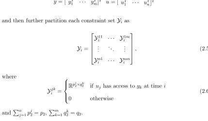
We can therefore partition the measured outputsyand control inputsuaccording to the dimension of the subsystems:

y= [ yT₁ _{· · ·} y_mT]T u= [ uT₁ _{· · ·} uT_n]T

and then further partition each constraint set _Yi as

Yi =

(31)

with communication delay τc between nodes. Then

where, for compactness, * is used to denote a space of appropriately sized real matrices.

In this setting, every decision maker then has access to all measurements that are at

least 2τc time-steps old.

The distributed control problem of interest is to design a controller K _{∈ S} so as to achieve a pre-defined closed loop_H∞ norm. Specifically, the problem is to find an internally stabilizing K _{∈ S} such that

||P₁₁+P₁₂K(I₋P₂₂K)−1P₂₁_||∞_≤γ (2.9)

for some pre-defined γ > γinf, where γinf is the optimal achievable closed loop H∞

norm.

(32)

Definition 2.1 A set _S is quadratically invariant under P22 if

KP22K ∈ S for all K ∈ S

In [9], it was shown that if _S is quadratically invariant under P22, then K ∈ S

if and only if Q = K(I ₋P22K)−1 ∈ S. In the case of delay-constraints imposed

by a communication graph, intuitive and easily verifiable conditions for QI can be stated [10]. Essentially these conditions say that in order to have QI, controllers must be able to communicate with each other faster than their control actions propagate through the plant – this is closely related to funnel causality [25], partial nestedness [8] and poset causality [14].

Thus, if quadratic invariance holds, the feasibility problem (2.9) can be reduced, via the Youla parameterization, to the following equivalent model matching problem:

Problem 2.1 Find Q_{∈ S} T_RH∞ such that

||T1− T2QT3||∞ ≤γ (2.10)

for some γ > γinf, with T1 =P11, T2 =P12 and T3 =P21.

2.3

A Review of “1984”

H

_∞

Control

As our solution is based on the so-called “1984” approach to _H∞ control, we review it in this section. The following is based on material found in chapter 8 of [53].

2.3.1

T

₃

=

I

Case

We begin with the solution to the sub-optimal model matching problem with_T3 =I

(33)

Problem 2.2 Find Q _{∈ RH∞} such that _kT1 − T2Qk∞ ≤ γ for some γ > γinf ≥ 0,

where γinf is the optimal achievable closed loop H∞ norm.

In order to state the main result, we first define the following transfer matrices: 1. LetUi, Uo be an inner-outer factorization ofT2 such that T2 =UiUo, with Ui∼Ui =

I, andUi, Uo, Uo†∈ RH∞.

2. Let Y := (I₋UiUi∼)T1.

3. For γ > _kY_k∞, let Yo be a bi-stable spectral factor of γ2I − Y∼Y such that γ2I₋Y∼Y =Y_o∼Yo, with Yo, Yo−1 ∈ RH∞.

4. Define the _RL∞ matrix R:=U_i∼_T1Yo−1.

Theorem 2.1 Let α := inf_{kT1− T2Qk∞ : Q∈ RH∞}. Then

1. α= inf_{γ : _kY_k∞< γ, dist (R,_RH∞)<1_}, and

2. For γ > α and Q, X _{∈ RH∞} such that

• kR₋X_k∞ _≤1, and

• X =UoQYo−1,

we have that _kT1− T2Qk∞≤γ.

Before proving this result, we need the following two preliminary lemmas:

Lemma 2.1 Let U be inner and E _{∈ RL∞} be given by

E :=



 U∼

I₋U U∼



.

(34)

Lemma 2.2 For F, G_{∈ RL∞} with the same number of columns, if

Lemma 2.3 (Nehari’s Theorem) For any R_{∈ RL∞}, we have that

dist (R,_RH∞) = dist (R,_H∞) =_kΓRk,

and that there exists X _{∈ RH∞} such that _kR₋X_k∞= dist (R,_RH∞).

(35)

Applying Lemma 2.2, this then implies that

kY_k∞< γ, (2.15)

and

kU_i∼T1Yo−1−UoQYo−1k∞ <1 (2.16)

By Lemma 2.3, this in turn implies that dist (R, Uo(RH∞)Yo−1) < 1, which, noting

that Uo is right invertible in RH∞ and thatYo is invertible inRH∞, is equivalent to

dist (R,_RH∞)<1 (2.17)

Then, from (2.15) and (2.17), and the definition of γinf we conclude that γinf ≤ γ,

and thus that γ < α+. Since was arbitrary, we then have that γ_inf _≤α.

To prove the reverse inequality, again choose > 0 and γ such that γinf < γ <

γ_inf +. Then (2.15) and (2.17) hold, so (2.16) holds for some Q_{∈ RH∞}. Applying the converse of Lemma 2.2, this in turn implies that



Ui∼T1−UoQ Y

 

∞

≤γ. (2.18)

Finally, reversing the above steps, this leads to _kT₁_{− T}₂Q_k∞ _≤ γ. Thus α _≤ γ < γinf +, and hence α≤γinf.

2) This follows immediately from the previous derivation.

Thus, a high level outline for computing an_H∞ controller satisfying a γ bound in closed loop is

1. Compute Y and _kY_k∞.

2. Select a trial value γ >_kY_k∞.

3. ComputeRand_kΓRk. Then kΓRk<1if and only ifα < γ, so increase or decrease γ accordingly, and return to step 2 until a sufficiently accurate upper bound for α

(36)

4. Find a matrix X _{∈ RH∞} such that_kR₋X_k∞_≤1.

5. Solve X =UoQYo−1 for aQ∈ RH∞ satisfying kT1− T2Qk∞ ≤γ.

2.3.2

General

T

₃

We now state the result for general _T3. First, define the following matrices

1. LetUi, Uo be an inner-outer factorization ofT2 such that T2 =UiUo, with Ui∼Ui = I, andUi, Uo, Uo†∈ RH∞.

2. Let Y := (I₋UiUi∼)T1.

3. For γ > _kY_k∞, let Yo be a bi-stable spectral factor of γ2I − Y∼Y such that γ2I₋Y∼Y =Y_o∼Yo, with Yo, Yo−1 ∈ RH∞.

4. Let Vco, Vci be a co-inner-outer factorization of T3Yo−1 such that T3Yo−1 = VcoVci

and V_ci, V_co, V_co† _{∈ RH∞}.

5. Let Z :=U_i∼_T1Yo−1(I−Vci∼Vci).

6. If _kZ_k∞ < 1, let Z_co be a bi-stable co-spectral factor of I ₋ZZ∼ such that I ₋ ZZ∼ =ZcoZco∼, with Zco, Zco−1 ∈ RH∞.

7. Let R:=Z_co−1U_i∼_T1Yo−1Vci∼.

Theorem 2.2 Let α := inf_{kT1− T2QT3k∞:Q∈ RH∞}. Then

1. α= inf_{γ : _kY_k∞ < γ,_kZ_k∞ <1, dist (R,_RH∞)<1_}, and

2. For γ > α and Q, X _{∈ RH∞} such that

• kR₋X_k∞ _≤1, and

• X =Z_co−1UoQVco,

(37)

Proof: Analogous from that of Theorem 2.1, and therefore omitted.

Similarly, we may outline a general high level algorithm for computing a controller using Theorem 2.2:

2. Select a trial value γ >_kY_k∞. 3. Compute Z and _kZ_k∞.

4. If _kZ_k∞ <1, continue; if not, increaseγ and return to step 3.

5. ComputeRand_kΓRk. Then kΓRk<1if and only ifα < γ, so increase or decrease γ accordingly, and return to step 3 until a sufficiently accurate upper bound for α

is obtained.

6. Find a matrix X _{∈ RH∞} such that_kR₋X_k∞_≤1.

7. Solve X =Z_co−1UoQVco for a Q∈ RH∞ satisfying kT1− T2QT3k∞≤γ.

2.4

Distributed

H

_∞

Control Subject to Delays

As in [16], we exploit the fact that the communication graph is strongly connected to decompose Q into a local distributed FIR filter V _{∈ Y} and a global, but delayed, IIR component ∆_ND_∈ _z1NRH∞, where in particular,D ∈ RH∞ is unconstrained:

Q=V + ∆D_{∈ S}, with V _{∈ Y}, D _{∈ RH∞} (2.19)

We will show that when Q admits such a decomposition, the norm bound test of Theorem 2.1 reduces to verifying the existence of a FIR filter V _{∈ Y} such that kΓ_Rˆ₍_V₎k <1, where R(Vˆ ) is a transfer matrix to be defined that depends affinely on

(38)

2.4.1

T

₃

=

I

Case

We begin with a solution to the_T3 =I case to simplify the exposition, as the general

case, much as in the centralized problem, follows from an analogous argument. Let

• Tˆ1(V) :=T1− T2V,

• Tˆ2 :=T2∆N,

• Uî :=Ui∆N,Uô =Uo ∈ RH∞be inner and outer, respectively, such thatTˆ2 = ÛiUô,

and Uˆ_o−1 _{∈ RH∞}.

• R(Vˆ ) := ∆∼_NR₋Uˆo(∆∼NV)Yo−1,

with Y_o−1 and R defined as in Section 2.3.1. We then have that

Theorem 2.3 Let α := inf_{k_Tˆ1(V)−Tˆ2Dk∞ : D∈ RH∞, V ∈ Y}. Then

1. α= inf_{γ : _kY_k∞< γ, _∃V _{∈ Y} s.t. distR(Vˆ ),_RH∞<1_}, and

2. For γ > α and D, X _{∈ RH∞} such that

• kR(Vˆ )₋X_k∞_≤1, and

• X = ˆUoDYo−1,

we have that _k_Tˆ1(V)−Tˆ2Dk∞≤γ.

Before proving this result, we will need the following lemma:

Lemma 2.4 For Yˆ(V) := (I₋UˆiUˆi∼) ˆT1(V), we have that Yˆ(V) =Y, where Y is as

defined in Section 2.3.1.

Proof: Straightforward, and thus omitted. We may now prove Theorem 2.3.

Proof: 1) Choose > 0 such that α < γ < α+, implying that there exists

(39)

We now proceed as in the proof of Theorem 2.1, and premultiply by

By Lemma 2.2 and Lemma 2.4, (2.21) is equivalent to

kY_k∞ < γ (2.22)

this is then equivalent to

kR(Vˆ )₋UˆoDYo−1k∞<1, (2.25)

which by the arguments of the proof of Theorem 2.1, is equivalent to _kΓ_Rˆ₍_V₎k<1.

The rest of the proof proceeds as that of Theorem 2.1.

Thus, for a fixed γ, we have reduced the problem to a feasibility test: does there exist a FIR filterV _{∈ Y} such that_kΓ_Rˆ₍_V₎k<1. As per identity (2.1), this is equivalent

(40)

Reduction to a LMI

LetR1 and R2 be an anti-stable/stable decomposition of∆∼NR. Now, define G(V)∈

RH∞ as

G(V) := UˆoV Yo−1 = P∞_i₌₀_z1iGi(V).

(2.26)

where the terms Gi(V) are the impulse response elements of G. It is easily verified

that these terms are affine in _{Vi}, the impulse response elements of V (i.e. V =

PN−1

i=0 z1iVi). Note that G(V)∈ RH∞ follows from Uo, V, Yo−1 ∈ RH∞. As such, let

G(V) :=



 AG BG

CG DG

 

be a minimal stable realization ofG. We then have that

ˆ

Uo∆∼NV Yo−1 = ∆∼NG

= zNP∞_i₌₀_z1iGi(V)

= PN_k₌₁zkGN−k(V) +P∞_j₌₀_z1jGj+N(V)

=: q(V)∼+NG(V).

(2.27)

with q(V) = PN_k₌₁_z1kG>_N₋_k(V)∈ RH∞ and strictly proper.

Also note that NG(V)has the following state space representation

NG(V) =



 AG BG

CGANG CGANG−1BG



, (2.28)

and is therefore also clearly in _RH∞.

The following lemma is an immediate consequence of the previous discussion.

(41)

ˆ

From our previous discussion, we have thus reduced the problem to finding an FIR filterV such that _kΓ˜_Rˆ₁₍_V₎k<1, for Rˆ1(V) given as in (2.29).

We begin by deriving a state space representation for Rˆ₁(V), and then use this representation to formulate the Hankel norm bound test as a LMI.

First note that q(V) is simply a strictly causal FIR filter, and thus has a state space representation given by

where Aq is the down-shift operator (i.e. a block matrix with appropriately

dimen-sioned Identity matrices along the first sub block diagonal, and zeros elsewhere),

Bq = [I, 0. . . , 0]>, and Cq(V) = [GN−1(V)>, . . . , G0(V)>]. Note that only Cq(V) is

a function of our design variable V.

Letting the strictly proper R1 ∈ RH∞ have a minimal stable realization

R₁ =

We emphasize again that our design variable V appears only in CR(V).

(42)

Proposition 2.1 For a system

F =



 A B

C 0



_{∈ RH∞},

we have that _kΓ˜Fk<1 if and only if there exist matrices P, Q≥ 0 and scalar λ≥0

such that _

A>QA−Q C>

C ₋λI



 _≤ 0

    

−P P B P A B>P ₋I 0 A>P 0 ₋P

   

 ≤ 0

P ₋Q _≥ 0 λ <1

(2.33)

Proof: This is the discrete-time analog of the variational formulation found in Section 6.3.1 of [55].

Substituting our realization (2.32) into (2.33), we see that this is an LMI in the variables_{Vi}iN=0−1,P,Q, andλ, and is feasible if and only if there exists an FIR filter

V _{∈ Y} such that _kΓ˜_Rˆ₁₍_V₎k<1.

Thus, a high level outline for computing a distributed controller satisfying an_H∞ norm bound of γ in closed loop is

(43)

3. ConstructRˆ1(V) and check if the LMI in variables {Vi}iN=0−1, Q, P and λ



A>RQAR−Q CR(V)> C_R(V) ₋λI



 _≤ 0

    

−P P B_R P A_R B_R>P ₋I 0 A>_RP 0 ₋P

   

 ≤ 0

P ₋Q _≥ 0 λ <1

(2.34)

is feasible forV =PN_i₌₀−1 _z1iVi ∈ Y. This LMI is feasible if and only ifkΓ˜_Rˆ₁₍_V₎k<1,

which in turn occurs if and only if α < γ, so increase or decrease γ accordingly. This feasibility test will additionally yield an FIR filter V _{∈ Y} that satisfies this bound.

4. Find a matrixX _{∈ RH∞}, implicitly dependent onV, such that_kR(Vˆ )₋X_k∞_≤1

(such a matrix is guaranteed to exist by the same arguments as those used in the centralized case).

5. Solve X = ˆUoDYo−1 forD ∈ RH∞ satisfying kTˆ1(V)−Tˆ2Dk∞≤γ.

6. Set Q=V + ∆ND∈ STRH∞

2.4.2

General

T

3

Define the following transfer matrices 1. Zˆ = ˆU_i∼_T1Yo−1(I−VciVci∼),

2. R(Vˆ ) := ∆∼_NR₋Z_co−1Uˆo(∆∼NV)Vco,

and letY_o−1, R,Vcoand Zco−1 be as defined in Section 2.3.2, andTˆ1(V), Tˆ2, Uˆi andUˆo

(44)

Theorem 2.4 Let α := inf_{k_Tˆ1(V)−Tˆ2DT3k∞:D∈ RH∞, V ∈ Y}. Then

1. α= inf_{γ : _kY_k∞< γ, _kZ_k∞ <1,_∃V _{∈ Y} s.t. dist

ˆ

R(V),_RH∞

<1_}, and

2. For γ > α and D, X _{∈ RH∞} such that

• kR(Vˆ )₋X_k∞_≤1, and

• X =Z_co−1UˆoDVco,

we have that _k_Tˆ1(V)−Tˆ2DT3k∞≤γ.

Proof: Analogous to that of Theorem 2.3, and therefore omitted.

Just as in the _T3 =I case, this problem has now been reduced to finding an FIR

filter V _{∈ Y} such that _kΓ˜_Rˆ₍_V₎k < 1. The arguments of the preceding section apply

nearly verbatim, with the exception of replacing equation (2.26) with

G(V) :=Z_co−1UˆoV Vco (2.35)

Therefore, a high level outline for computing a distributed controller satisfying an H∞ norm bound of γ in closed loop is

2. Select a trial value γ >_kY_k∞. 3. Compute Zˆ and _kZˆ_k∞.

4. If _kZˆ_k∞ <1, continue; if not, increaseγ and return to step 3.

5. ConstructRˆ1(V)according to (2.29), with G(V)defined as in (2.35), and check if

there exists V _{∈ Y} such that LMI (2.34) is feasible. This LMI is feasible if and only if _kΓ˜_Rˆ₁₍_V₎k < 1, which in turn occurs if and only if α < γ, so increase or

decrease γ accordingly. This feasibility test will additionally yield an FIR filter

(45)

6. Find a matrixX _{∈ RH∞}, implicilty dependent onV, such that_kR(Vˆ )₋X_k∞_≤1. 7. Solve X =Z_co−1UˆoDVco forD∈ RH∞ satisfying kTˆ1(V)−Tˆ2DT3k∞≤γ.

8. Set Q=V + ∆ND∈ STRH∞

2.5

Example

For the convenience of the reader, we provide explicit state-space formulae for the factorizations and approximations required to implement our algorithm in Section 2.7.

We consider a three-player chain with communication delay ofτc= 1– the sparsity

constraint _Y on the FIR filter is as given in equation (2.8). We first consider the simplified case of P21 =I – the remaining dynamics of P11, P12 and P22 are given by

Note that this is a suitably modified version of the output feedback problem considered in [16].

(46)

closed loop norm of .9772. This is a significant improvement over the delayed system (i.e.V0 andV1 constrained to be zero), for which we were only able to achieve a closed

loop norm of 1.6856.

We then considered the general output-feedback problem, with P21 given by the

parameters in (2.36) as well. The centralized and LMI computed centralized closed loop norms were both found to be 1.502, with the best distributed norm found to be 1.515. Once again, we see near identical performance from the centralized and distributed solutions, whereas the delayed controller was only able to achieve a closed loop norm of 2.213.

2.6

Conclusion

This chapter presented an LMI based characterization of the sub-optimal delay-constrained distributed _H∞ control problem. By exploiting the strongly connected nature of the communication graph, we were able to reduce the problem to a feasi-bility test in terms of the Hankel norm of a certain transfer matrix that is a function of the localized FIR component of the controller. We note that much as in the _H2

case, by reducing the control synthesis problem to one that is convex in the FIR filter, communication delay co-design [23,56] and augmentation [57] methods are applicable. However, although finite dimensional, this method is based on the “1984” approach to H∞ control – as such, the computational burden is quite high, limiting the scalability of the approach.

(47)

2.7

Factorization Formulas

In all of the following, we assume that the conditions needed for the existence of the required stabilizing solution of the corresponding Discrete Algebraic Riccati Equations (DARE) are met – the reader is referred to [2] and [58] for more details. All “co-X” factorizations, where ““co-X” may be either inner-outer or bi-stable spectral, can be obtained by transposing the “X” factorization of the transpose system.

2.7.1

Inner-Outer Factorizations

Let

G:=



 A B

C D



_{∈ RH∞}.

From [2], an inner-outer factorization G=UiUo of G, with Ui inner and Uo outer, is

given by

U_i =



 A+BF BH−1

C+DF DH−1



 (2.37)

Uo =



 A B

−HF H



 (2.38)

with H = (D>D+B>XB)12, and X the stabilizing solution of the following DARE

X = A>XA+C>C+A>XBF, F = ₋(D>D+B>XB)−1B>XA.

(2.39)

2.7.2

Bi-stable Spectral Factorizations

LetY _{∈ RH∞} be strictly proper, and let

GY =



 AY BY

CY 0

 

(48)

If AY is invertible, then it holds that

γ2I₋Y∼Y =GY +G∼Y +DY +DY>

where DY = 1₂ γ2I+BY>A−>Y CY>

.

A bi-stable spectral factorization γ2I ₋Y∼Y =M∼M, with M, M−1 _{∈ RH∞} is then given by

M =



 AY BY

H−1(CY +BY>XAY) H



 (2.40)

with H = (DY +DY>+BY>XBY)

1

2, and X the stabilizing solution of the following DARE

X = A>_YXAY + (A>YXBY +CY>)F,

F = ₋(D>_Y +DY +BY>XBY)−1(BY>XAY +CY).

(2.41)

This result follows directly from standard results on spectral factors and positive real systems [2]

2.7.3

Stable Approximations

The following is taken from [58]. Let

G:=



 A B

C D



_{∈ RH∞}

be a minimal state-space representation, and assume that ρ=_kΓ˜Gk< γ. Let X and Y be the controllability and observability Gramians of G, respectively.

Let Q_{∈ RH∞} have the state-space representation

Q:=



 AQ BQ

C_Q D_Q

 

(49)

A_Q =A₋BC_Q, B_Q =AXC>+BE>, CQ = (E>C+B>Y A)N, DQ =D>−E>,

where N = (γ2I₋XY)−1, and for any unitary matrix U,

E =₋(I +CN XC>)−1CN XA>Y B

+γ(I+CN XC>)−21U(I+B>Y N B)− 1 2.

(50)

Chapter 3

Optimal Two Player LQR State

Feedback with Varying Delay

3.1

Introduction

As described in Section 2.1, quadratic invariance has spurred on a flurry of activ-ity in distributed optimal control synthesis subject to sparsactiv-ity and delay constraints. However, an underlying assumption in the aforementioned results is that information, albeit delayed, can be transmitted perfectly across a communication network with a

fixed delay. A realistic communication network, however, is subject to data rate lim-its, quantization, noise and packet drops – all of these issues result in possibly varying delays (due to variable decoding times) and imperfect transmission (due to data rate limits/quantization). The assumption that these delays are fixed necessarily intro-duces a significant level of conservatism in the control design procedure. In particular, to ensure that the delays under which controllers exchange information do not vary, worst case delay times must be used for control design, sacrificing performance and robustness in the process.

(51)

results exist, however, that seek to combine NCS and decentralized optimal control. A notable exception is the work by [62], in which an explicit state space solution to a sparsity constrained two-player decentralized LQG state-feedback problem over a TCP erasure channel is solved.

Chapter contributions: We take a different view from these results, and sup-press the underlying details of the communication network, and instead assume that packet drops, noise, and congestion manifest themselves to the controllers as varying delays. Indeed, as shown in [63], delays play a dominant role in determining closed-loop performance relative to channel issues such as quantization. In particular, we seek to extend the distributed state-feedback results of [39, 64] and [15] to accom-modate varying delays. In addition to allowing for communication channels to be more explicitly accounted for in the control design procedure, the ability to accom-modate varying delays provides flexibility in the coding design aspect of this problem – we are currently exploring the application of deadline based coding schemes devel-oped by [65], initially designed for real-time video streaming, to optimal decentralized control.

In this chapter, we focus on a two plant system in which communication between controllers occurs across a communication link with varying delay. We extend the dynamic programming methods in [39] and [15] to accommodate this varying delay, and show that under suitable assumptions, the optimal control actions are linear in their information, and that the resulting controller has piecewise linear dynamics dictated by the current effective delay regime. The results in this chapter were first presented in [18, 19].

(52)

3.2

Problem Formulation

We begin by describing the general problem of interest, and then specialize the for-mulation to the particular case to be addressed in this paper.

Notation

For a matrix partitioned into blocks

M = process r_0:_t, we denote the conditional probability of an event _A occurring given this history by _Pr0:t(A). If Y = {y

1_{, . . . , y}M_} _{is a set of random vectors (possibly of}

different sizes), we say that z _∈lin (_Y)if there exist appropriately sized real matrices

C1, . . . , CM such that z =PM_i₌₁Ciyi.

3.2.1

The two-player problem

This paper focuses on a two plant system with physical propagation delay of D

between plants, and varying communication delaysdi_t _{∈ {}0, . . . , D_}– to ease notation, we letd_t := (d1_t, d2_t). We impose some additional assumptions on the stochastic process

dt in Section 3.3 such that the infinite horizon solution is well defined.

(53)

x

1 1 2 3

x

2

Figure 3.1: The distributed plant considered in (3.6), shown here forD= 4. Dummy nodes δ_ti, i = 1, . . . , D₋1, as defined by (3.5), are introduced to make explicit the propagation delay ofD between plants.

equation:

xi_t₊₁ = Aiixit+Aijxj_t₋₍_D₋₁₎+Biuit+wti (3.1)

with mutually independent Gaussian initial conditions and noise vectors

xi₀ _{∼ N}(µi₀,Σ₀i), wi_t_{∼ N}(0, W_ti) (3.2)

We may describe the information available to controller i at time t, denoted by Ii

t, via the following recursion:

Ii

0 = {xi0}

Ii

t+1 = Iti∪ {xit+1} ∪ {x

j

k : 1≤k ≤t+ 1−d j t+1}

(3.3)

The inputs are then constrained to be of the form

ui_t = γ_ti(_I_ti) (3.4)

for Borel measurable γ_ti.

In order to build on the results in [15], we model the two plant system as a

D+ 1 node graph, with “dummy delay” nodes introduced to explicitly enforce the propagation delay between plants. Specifically, letting

δi_t=



 x1t−i x2_t₋₍_D₋_i₎



, i= 1, . . . , D₋1 (3.5)

(54)

{1_} the information in the label set is, and (iii) that _LV_t contains all of the information at nodes s.t. _|s_| > ei_t, s ₃ i. We also see that the graph is naturally divided into two branches, with each branch corresponding to information pertaining to a specific plant.

representation for the system

xt+1 =Axt+But+wt (3.6)

where, to condense notation, we let

x=

and A and B are such that (3.6) is consistent with (3.1) and (3.5). The physical topology of the plant is illustrated in Figure 3.1.

Problem 3.1 Given the linear time invariant (LTI) system described by (3.1), (3.5) and (3.6), with disturbance statistics (3.2), minimize the infinite horizon expected cost

(55)

subject to the input constraints (3.4).

The weight matrices are assumed to be partitioned into blocks of appropriate dimension, i.e. Q = (Qij) and R = (Rij), conforming to the partitions of x and u. We assume Q to be positive semi-definite, and R to be positive definite, and in order to guarantee existence of the stabilizing solution to the corresponding Riccati equation, we assume (A, B) to be stabilizable and (Q12, A)to be detectable.

3.3

Main Result

3.3.1

Effective delay

The information constraint sets (3.3) are defined in such a way that controllers do not forget information that they have already received. This leads to the xj component of the information set_I_ti being a function of theeffective delay seen by the controller, as opposed to the current delay value of the communication channel dj_t.

Definition 3.1 Let

ej_t := min_{dj_t, dj_t₋₁ + 1, dj_t₋₂ + 2, . . . , d_tj₋₍_D₋₂₎+ (D₋2), d_tj₋₍_D₋₁₎ + (D₋1)_} (3.9)

be the effective delay in transmitting information from controller j to controller i.

Lemma 3.1 The information set available to controller i at time t may be written as

Ii

t =Iti−1∪ {xit} ∪ I j

t−ej_t (3.10)

Proof: See §3.6.

In order to ensure that the infinite horizon solution is well defined, we assume that

lim T→∞

1 T

T−1

X

t=0

Pd0:t e

i t+1 ≤d

(56)

exists for any integerd, i.e. we assume that the asymptotic distribution ofei, condi-tioned on its history, is stationary and well defined.

3.3.2

Partial Nestedness

Here we show that the information constraints (3.4) and system (3.6) are partially nested (c.f. [8]), and hence that the optimal control policies γ_ti are linear in their information set.

Definition 3.2 A system (3.6) and information structure (3.4) is partially nested if, for every admissible policy γ, whenever ui_τ affects _I_tj, then _I_τi _{⊂ I}_tj.

Lemma 3.2 (see [8]) Given a partially nested information structure, the optimal control law that minimizes a quadratic cost of the form (3.8) exists, is unique, and is

linear.

Using partial nestedness, the following lemma shows that the optimal state and input lie in the linear span of _I_ti and _Ht, where Ht is the noise history of the system

given by

Ht={x0, w0:t−1} (3.12)

Lemma 3.3 The system (3.6) and information structure (3.4) is partially nested, and for any linear controller, we have that

xi_t, ui_t _∈lin _I_ti x_t, u_t_∈lin (_H_t) (3.13)

(57)

3.3.3

Information Graph and Controller Coordinates

Lemma 3.3 indicates that each _I_ti is a subspace of _Ht: in this section, we exploit

this observation to define pairwise independent controller coordinates. An explicit characterization of these subspaces is given in Section 3.4.

We begin by defining the information graph, as in [15], associated with system (3.6) by _G = (_V,_E), with

V := _{1_},_{1, δ1_}, . . . ,1, δ1, . . . , δD−1 _∪

{2_},δD−1,2 , . . . ,δ1, . . . , δD−1,2 _∪V

E := _{(r, s)_{∈ V × V} : _|s_|=_|r_|+ 1_{} ∪ {}(V, V)_}

(3.14)

where V :=1, δ1, . . . , δD−1,2 . For the case of D = 4, the graph _G is illustrated in Figure 3.2.

Before proceeding, we define the following sets, which will help us state the main result. Let

vi,_t+ := _{s _{∈ V\}V _|i_∈s, _|s_{| ≥}ei_t_} v_ti,++ := _{s _{∈ V\}V _|i_∈s, _|s_|> ei_t_}

(3.15)

and similarly define v_ti,− and v_ti,−− as in (3.15), but with the (strict) inequality re-versed.

Theorem 3.1 Consider Problem 3.1, and let _G(_V,_E) be the associated information graph. Let

XV = Q+A>XVA+A>XVBKV KV := ₋ R+B>XVB−1B>A,

(3.16)

be the stabilizing solution to the discrete algebraic Riccati equation, and the centralized

(58)

node such that (r, s)_{∈ E}. Define the matrices

The optimal control decisions then satisfy

ζ_tV₊₁ = Aζ_tV +BϕV_t +

and the corresponding infinite horizon expected cost is

2

X

i=1

Trace X{i}Wi (3.20)

Proof: See Section 3.4.

(59)

mechanism is in place such that the et is known to both players; relaxing this

assump-tion will be the subject of future work.

Remark 3.2 The probabilities pr and qr can be computed directly if we assume the

{pi,d_t _} to be independently and identically distributed. In this case, ej_t evolves accord-ing to an irreducible and aperiodic Markov chain with transition probability matrix

computable directly from the definition of effective delay and the pmf of dt. As such,

pr and qr can be computed from the chain’s stationary distribution, which is

guaran-teed to exist. Future work will explore what additional distributions on dt will lead to

closed form expressions for pr andqr. Failing the existence of closed form expressions

for these asymptotic distributions, computing estimates via simulation should be a

feasible option for many interesting pmfs _{pi,d_t _} .

3.4

Controller Derivation

3.4.1

Controller States and Decoupled Dynamics

As mentioned previously, each _I_ti is a subspace of _Ht: in this section, we aim to

explicitly characterize these subspaces by assigning label sets _{Ls_0:_t_}s∈V to the graph G = (_V,_E)as defined by (3.14). In particular, they are defined recursively as:

Ls

0 = ∅, for |s|>1

Li

0 = {xi0}

Li

t+1 = {wit}

Ls

t+1 = Lrt, for (r, s)∈ E, 1<|s|< D+ 1

LV

t+1 = LVt ∪i∪_s_∈_vi,+

t+1L

s t

(3.21)

where we have let _∪i denote∪2i=1 to lighten notational burden. An example of these

label sets for the case of D= 4 is illustrated in Figure 3.2.

(60)

spreading. As can be seen in Figure 3.2, for each(r, s)_{∈ E}, with_|r_|< D+ 1, we have that _|s_| = _|r_|+ 1, and additionally, that _|s_| corresponds exactly to how delayed the information in the label set is. We also see that the graph is naturally divided into twodisjoint branches, with each branch corresponding to information about a specific plant. Finally, the label corresponding to the root node V can be interpreted as the information available to both controllers – this is reflected by its explicit dependence on the effective delay ei_t.

Remark 3.3 Note that in contrast to [15], the label sets as defined will in general

not be disjoint. However, as will be made explicit in Lemma 3.5, an effective delay dependent subset of the label sets will indeed form a partition (i.e. a pairwise disjoint

cover) of the noise history.

We may now characterize the subspaces of _Ht that are associated with each Iti.

This characterization will be shown to depend on the effective delay ej_t seen at node

i, and will lead to an intuitive partitioning of both the state and the control input. We begin by pointing out the following useful facts that will be used repeatedly in the derivation to come

Lemma 3.4 Let v_ti,∗, _{∗ ∈ {−},_−−}, be given as in (3.15). Then, for a fixed i, we have that

∪s∈vi,_t₊₁− L s

t+1 =∪r∈vi,_t₊₁−−L r

t ∪ Lit+1, (3.22)

and for integers a, b_{∈ {}0, . . . , D₋1_}

∪a<|s|≤b+1Lst+1 =∪a≤|r|≤bLrt (3.23)

Proof: Follows i

Distributed Optimal Control of Cyber Physical Systems: Controller Synthesis, Architecture Design and System Identification

Systems: Controller Synthesis, Architecture Design

Contents

List of Figures

List of Tables

Chapter 1

Non-Classical Information Sharing Constraints

Thesis Contribution and Outline

Chapter 2

Problem Formulation

The model-matching problem subject to delay

V. NUMERICALEXAMPLES

A Review of “1984”

General

Distributed

CGANG CGANG−1BG

General

Example

Conclusion

Inner-Outer Factorizations

Stable Approximations

Chapter 3

Problem Formulation

The two-player problem

Main Result

Partial Nestedness

Information Graph and Controller Coordinates

Controller Derivation