R E S E A R C H
Open Access
A modified regularization method for an
inverse heat conduction problem with only
boundary value
Wei Cheng
1*and Yun-Jie Ma
2*Correspondence:
1College of Science, Henan
University of Technology, Zhengzhou, 450001, P.R. China Full list of author information is available at the end of the article
Abstract
This paper aims to solve an inverse heat conduction problem with only boundary value in a bounded domain, where the boundary data is given forx= 0. The solution is sought in the interval 0 <x≤1. The problem is seriously ill posed in the Hadamard sense. Using the Hölder inequality and some inequalities, a conditional stability is proved for this problem. A modified Tikhonov regularization method is proposed to recover the stability of the solution. An order optimal error estimate between the approximate solution and the exact solution is obtained with a suitable choice of regularization parameter. Numerical results are presented to illustrate the accuracy and efficiency of the proposed method.
MSC: 65M30; 35R25; 35R30
Keywords: ill-posed problem; inverse heat conduction problem; regularization; error estimate
1 Introduction
In this paper we consider the following inverse heat conduction problem with only bound-ary value:
ut=uxx, <x< , <t< π,
u(,t) =f(t), ≤t≤π, (.)
ux(,t) =g(t), ≤t≤π,
wheref andgare given. This problem is ill posed []. We want to recover the temperature distributionu(x,·) for <x≤ from the boundary dataf andg.
The inverse heat conduction problem (IHCP) arises from many physical and engineer-ing disciplines. It is well known that the problem is severely ill posed in the Hadamard sense that the solution (if it exists) does not depend continuously on the given data,i.e., a small measurement error in the given data can cause an enormous error in the solu-tion [–]. To overcome such difficulties, some regularizasolu-tion techniques are required []. The IHCP has been considered by many authors using different methods. These methods include the wavelet and wavelet-Galerkin method [–], the Tikhonov method [], the
mollification method [–], the fundamental solution method [], the Fourier method [], and so on.
To the best of the knowledge of the authors, the results available in the literature are mainly devoted to the IHCP with known initial-boundary value. However, in practical relife problems we cannot know the initial condition because the heat process has al-ready started before we estimate the problem. A few works are developed for the IHCP without initial value [, ]. Ginsberg [] used a cutoff method for an IHCP with only boundary value and gave a Hölder type error estimate. Recently, Liu and Wei [] used a quasi-reversibility regularization method for solving an IHCP without initial data. Yang and Fu [] applied a simplified Tikhonov regularization method for determining the heat source. In this paper, we will use a modified Tikhonov regularization method to deal with the IHCP without initial value (.) and obtain an order optimal error estimate between the approximate solution and the exact solution.
The paper is organized as follows. In Section , we give the formulation of the solu-tion for problem (.) and present some preliminary results. In Secsolu-tion , we prove the conditional stability for the IHCP (.) by using the Hölder inequality. Section proposes a modified Tikhonov regularization method. An order optimal error estimate for the ap-proximate solution is obtained with a suitable choice of regularization parameter. To verify the efficiency and accuracy of the proposed method for problem (.), we give two numer-ical examples in Section . A brief conclusion is given in Section .
2 Mathematical formulation and preliminaries
Throughout this paper, we use the following formulation and lemmas. For the IHCP (.), we want to determine the temperature distributionu(x,·) for <x≤ from the Cauchy dataf andg. Since the Cauchy dataf andg are measured, there will be measurement errors, and we would actually have measured Cauchy datafδ,gδ∈L[, π], for which
f –fδ≤δ, g–gδ≤δ, (.)
where the constant δ> represents a bound on the measurement error, · and (·,·) denote the norm and inner product onL[, π], respectively.
In the following, we split the IHCP (.) into two independent IHCPs:
vt=vxx, <x< , <t< π,
v(,t) =f(t), ≤t≤π, (.)
vx(,t) = , ≤t≤π,
and
wt=wxx, <x< , <t< π,
w(,t) = , ≤t≤π, (.)
wx(,t) =g(t), ≤t≤π.
Letv(x,t) andw(x,t) be the solution of problems (.) and (.), respectively. Thenu=
By the method of separation of variables, the exact solutions of problems (.) and (.) are given by
v(x,t) = +∞
n=–∞
f(t),einteintcosh(√inx) (.)
and
w(x,t) = +∞
n=–∞
√
in
g(t),einteintsinh(√inx). (.)
Then the exact solution of problem (.) is given by
u(x,t) = +∞
n=–∞
f(t),einteintcosh(√inx) +(g(t),e
int)
√
in e
intsinh(√inx)
. (.)
We assume also that there exists ana prioricondition for problem (.):
maxv(,·)p,w(,·)p ≤E, p≥, (.)
wherev(,·)p=
+∞
n=–∞( +n)p/(v(,·),ein(·))ein(·).
In order to give an error estimate for the regularized solution, we need the following lemma whose proof is similar to that of Lemma . in [].
Lemma . Let <x≤, < α< /e √
.We have the following inequalities:
sup
s≥
exs
+αes ≤α
–x, (.)
sup
s≥
e(+x)s( +s)–p +αes ≤α
–(+x)–ln(α)–pp+
. (.)
We need also the following results.
Lemma . Let <x≤,then there holds[]:
lim
n→o
sinh(√inx) √
in =x,
sinh√(√inx)
in
≤√xe
|n|
x, n∈Z, (.)
cosh(√inx)≤e
|n|
x, sinh(√inx)≤e
|n|
x, n∈Z, (.)
cosh(√in)≥ce
|n|
, sinh(√in)≥ce
|n|
, |n| ∈N+, (.)
where c= ( –e–√)/.
3 Conditional stability
Theorem . Let the a priori bound(.)hold and v(x,t)be the solution of problem(.)
given by(.)with the exact data f(t),then for a fixed x∈(, )the following estimate holds:
v(x,·)≤c–xExf–x. (.)
Proof By the Hölder inequality and (.), we have
v(x,·)=
+∞
n=–∞
cosh(√inx)f,ein(·)ein(·)
= +∞
n=–∞
cosh(√inx)|fn|
= +∞
n=–∞
cosh(√inx)|fn|x
|fn|(–x)
≤
+∞
n=–∞
cosh(√inx)|fn|x
x
x+∞
n=–∞
|fn|(–x)
–x
–x
=
+∞
n=–∞
cosh(√inx)
x|f
n|
x +∞
n=–∞ |fn|
–x
=
+∞
n=–∞
cosh(√inx)
xcosh(√in)–v(,·),ein(·)
x
f(–x)
≤
+∞
n=–∞
cosh(√inx)xcosh(√in)– +np
v(,·),ein(·)
x
f(–x)
≤max
n∈Zcosh(
√
inx)cosh(√in)–xv(,·)pxf(–x).
Using (.) and (.), we have
cosh(√inx)cosh(√in)–x≤e√|n|/xce√|n|/–x=c–x, |n| ∈N+,
then we get
max
n∈Z
cosh(√inx)cosh(√in)–x=max
n∈Z
,max
n∈N+
|cosh(√inx)| |cosh(√in)|x
≤c–x.
Combining with thea prioribound (.), we obtain
v(x,·)≤c–xExf(–x).
The proof is completed.
Remark . Ifv(x,t) andv(x,t) are the solutions of problem (.) with the exact data
f(t) andf(t), respectively, then for a fixedx∈(, ) we have
v(x,·) –v(x,·)≤c–xExf(·) –f(·) –x
. (.)
Theorem . Suppose that w(x,t)is the solution of problem(.)given by(.)with the exact data g(t)and the a priori bound(.)is valid,then for a fixed x∈(, )the following estimate holds:
w(x,·)≤c–x(√x)–xExg–x. (.)
Proof Using the Hölder inequality and (.), we have
w(x,·)=
+∞
n=–∞
sinh(√inx) √
in
g,ein(·)ein(·)
= +∞
n=–∞
sinh√(√inx)
in
|gn|
= +∞
n=–∞
sinh(√inx)/√in|gn|x
|gn|(–x)
≤
+∞
n=–∞
sinh(√inx)/√in|gn|x
x
x+∞
n=–∞ |gn|
–x
=
+∞
n=–∞
sinh√(√inx)
in
x
sinh√(√in)
in
–w(,·),ein(·)
x
g(–x)
≤
+∞
n=–∞
sinh√(√inx)
in
x
sinh√(√in)
in
– +npw(,·),ein(·)
x
g(–x)
≤max
n∈Z
sinh√(√inx)
in
sinh√(√in)
in
–xw(,·)pxg(–x).
From (.)-(.), we get
sinh√(√inx)
in
sinh√(√in)
in
–x=sinh( √
inx) √
in
(–x)sinhsinh((√√inx)
in)
x
≤√xe√|n|/x(–x)
e√|n|/x ce√|n|/
x
=c–x(√x)(–x), |n| ∈N+,
so
max
n∈Z
sinh√(√inx)
in
sinh√(√in)
in
–x=max
n∈Z
x,max
n∈N+
|(sinh(√inx))/√in| |(sinh(√in))/√in|x
≤c–x(√x)(–x).
Combining with (.), we obtain
w(x,·)≤c–x(√x)(–x)Exg(–x).
Estimate (.) is proved.
Remark . Ifw(x,t) andw(x,t) are the solutions of problem (.) with the exact data
g(t) andg(t), respectively, then for a fixedx∈(, ) we have
w(x,·) –w(x,·)≤c–x(√x)(–x)Exg(·) –g(·) –x
From Theorems . and ., we then obtain the following theorem.
Theorem . Let the a priori bound(.)hold and u(x,t)be the solution of problem(.)
given by(.)with the exact data f(t)and g(t),then for a fixed x∈(, )we have the fol-lowing estimate:
u(x,·)≤c–xExf–x+c–x(√x)–xExg–x. (.)
Remark . Ifu(x,t) andu(x,t) are the solutions of problem (.) with the exact data
pairs [f(t),g(t)] and [f(t),g(t)], respectively, then for a fixedx∈(, ) we get
u(x,·) –u(x,·)≤c–xExf(·) –f(·) –x
+c–x(√x)(–x)Exg(·) –g(·) –x
. (.)
4 Regularization and error estimates
Since Cauchy problems (.) and (.) are all severely ill posed, we should apply a regular-ization method to solve them.
4.1 Regularization and error estimate for problem (2.2)
For problem (.), we define an operator K :v(x,·)→f(·), then problem (.) can be rewritten as the following operator equation:
Kv(x,t) =f(t), <x≤. (.)
Combining with equation (.), we have
Kv(x,t) = +∞
n=–∞
v(x,t),eintcosh(√inx)–eint. (.)
Consequently,Kis an operator with eigenvalues
kn=
cosh(√inx)–. (.)
For disturbed datafδ(t), we use the Tikhonov regularization method, which seeks a
func-tionvδ
α(x,·) from minimizing quadratic functional
Jαvδ:=Kvδ–fδ+αvδ. (.)
According to Theorem . of [], this Tikhonov functional Jα has a unique minimum
vδ
α(x,·) which is the unique solution of the normal equation
K∗Kvδα+αv δ α=K∗f
δ
, α> , (.)
hereK∗is the adjoint ofK. Using the properties of the inner product, we obtain the eigen-values of operatorK∗:
kn=
where the symbol h(·) denotes the complex conjugate of the functionh(·). Combining (.), (.), (.) with (.), we get
+∞
n=–∞
knkn+α
vδα(x,t),eint
eint= +∞
n=–∞ kn
fδ(t),einteint.
This yields
vδ α(x,t) =
+∞
n=–∞
vδ α(x,t),e
inteint=
+∞
n=–∞ kn
|kn|+α
fδ(t),einteint
= +∞
n=–∞
cosh(√inx)
+α|cosh(√inx)|
fδ(t),einteint. (.)
We callvδ
α(x,t) given by (.) the Tikhonov approximate solution of problem (.). In
or-der to or-derive the error estimate between the regularized solution and the exact solution, we replace the original filter
+α|cosh(√inx)| with another filter +α|cosh(√in)|. Thus, the
modified regularized solution of problem (.) becomes
vδα,∗(x,t) :=
+∞
n=–∞
cosh(√inx)
+α|cosh(√in)|
fδ(t),einteint. (.)
We then have an error estimate for the modified Tikhonov approximate solution of prob-lem (.).
Theorem . Let v(x,t)given by(.)and vδ,∗
α (x,t)given by(.)be the exact solution and modified Tikhonov regularization solution of problem(.),respectively.Suppose that the noisy data fδ(t)satisfies(.)and the a priori condition(.)is valid.If < α< /e√and
we select the regularization parameterαas
α= (δ/E)ln(E/δ)
p
p+, (.)
then for a fixed x∈(, ],we have the following stability estimate:
v(x,·) –vδα,∗(x,·)≤c–xExδ–x
lnE δ
–p
p+x
+c–+o(), δ→ (.)
Proof By using the triangle inequality, with (.) and (.), we have
v(x,·) –vδ,∗ α (x,·)=
+∞
n=–∞
kn–f,ein(·)– (f
δ,ein(·))
+α|cosh(√in)|
ein(·)
≤ +∞
n=–∞
kn–α|cosh(√in)| +α|cosh(√in)|
f,ein(·)ein(·)
+ +∞
n=–∞
k–
n
+α|cosh(√in)|
f–fδ,ein(·)ein(·)
≤αsup
n∈Z
|cosh(√inx)cosh(√in)|( +n)–p +α|cosh(√in)|
× +∞
n=–∞
+|n|
p
v(,·),ein(·)ein(·)
+sup
n∈Z
|cosh(√inx)| +α|cosh(√in)|
+∞
n=–∞
f –fδ,ein(·)ein(·)
=αsup
n∈Z
A(n)v(,·)p+sup
n∈Z
B(n)f –fδ,
where
A(n) =|cosh( √
inx)cosh(√in)|( +n)–p
+α|cosh(√in)| , B(n) =
|cosh(√inx)| +α|cosh(√in)|.
Lets=√|n|/. Using the inequalities (.)-(.) and (.), we can get
B(n) = |cosh( √
inx)| +α|cosh(√in)| ≤
e√|n|/x
+ (cα)e√|n| = exs
+ (cα)es≤(cα)
–x, |n| ∈N+.
Thus, we have
sup
n∈Z
B(n) =max
+α,|sup
n|∈N+
|cosh(√inx)| +α|cosh(√in)|
=max
+α, (cα)
–x
= (cα)–x. (.)
Analogously, we can estimatesupn∈ZA(n). From the inequalities (.)-(.) and (.), we get
A(n) =|cosh( √
inx)cosh(√in)|( +n)–p +α|cosh(√in)| ≤
e√|n|/(x+)( +n)–p + (cα)e√|n|
≤e(x+)s( +s)– p
+ (cα)es ≤(cα)
–(x+)
ln α
–pp+
, |n| ∈N+.
Then we have
sup
n∈ZA(n) = max
+α, (cα)
–(x+)
ln α
–pp+
= (cα)–(x+)
ln α
–pp+
. (.)
Combining with (.)-(.), conditions (.), (.) and the choice ofαgiven by (.), we obtain
v(x,·) –vδα,∗(x,·)≤c–(x+)α–x
ln α
–pp+
E+ (cα)–xδ
≤c–(x+)E
δ E lnE δ p
p+–x
ln E δ lnE δ
+
cδ
E
lnE δ
p
p+–x
δ
=c–xExδ–x
lnE δ
–p
p+x
c–
lnE δ
lnEδ–pp+ln(lnEδ)
p
p+
+
.
Note that ln(E/δ)
lnEδ–pp+ln(lnEδ)→ forδ→. The proof is completed.
4.2 Regularization and error estimate for problem (2.3)
For problem (.), the Tikhonov method involves minimizing the quadratic functional:
Twδ–gδ+αwδ, (.)
whereT:w(x,·)→g(·) is a forward operator. We know that the above Tikhonov functional has a unique minimumwδ
α(x,·) which is the unique solution of the normal equation
T∗Twδα+αw δ α=T∗g
δ
, α> . (.)
We can obtain the Tikhonov regularized solution of problem (.):
wδα(x,t) =
+∞
n=–∞
t–n
+α|sinh√(√inx)
in |
gδ(t),einteint, (.)
where tn = √
in
sinh(√inx) is the eigenvalues of operator T. Similarly, we use the filter
+α|sinh(√in)| to replace the original filter
+α|sinh√(√inx)
in |
. Therefore, we get the modified
regularized solution of problem (.):
wδ,∗ α (x,t) =
+∞
n=–∞
t–
n
+α|sinh(√in)|
gδ(t),einteint. (.)
Theorem . Suppose that w(x,t)is the exact solution given by(.),and wδ,∗
α (x,t)given by(.)is the modified Tikhonov regularization solution of problem(.).Let the noisy data gδ(t)satisfy(.)and the a priori condition(.)be valid.If < α< /e√and the
regularization parameter is given by(.).Then for a fixed x∈(, ],we have
w(x,·) –wδα,∗(x,·)≤c–xExδ–x
lnE δ
–p
p+x√
x+c–+o(), δ→. (.)
Proof By using the triangle inequality, with (.) and (.), we have
w(x,·) –wδ,∗ α (x,·)=
+∞
n=–∞
t–n g,ein(·)– (g
δ,ein(·))
+α|sinh(√in)|
ein(·)
≤αsup
n∈Z
|sinh(√inx)sinh(√in)|( +n)–p +α|sinh(√in)|
× +∞
n=–∞
+|n|
p
w(,·),ein(·)ein(·)
+sup
n∈Z
|(sinh(√inx))/√in|
+α|sinh(√in)|
+∞
n=–∞
g–gδ,ein(·)ein(·)
=:αsup
n∈ZC(n)
w(,·)p+sup
n∈ZD(n)
f–fδ.
Using the methods dealing withsupn∈ZA(n) andsupn∈ZB(n), with (.)-(.), (.), and (.), we obtain
sup
n∈Z
C(n)≤(cα)–(x+)
ln α
–pp+
, sup
n∈Z
D(n)≤√x(cα)–x. (.)
Combining with (.), conditions (.), (.), and the choice ofαgiven by (.), we get
w(x,·) –wδα,∗(x,·)≤c–(x+)α–x
ln α
–pp+
E+√x(cα)–xδ
≤c–xExδ–x
lnE δ
–p
p+x
c–
lnE δ
lnEδ–pp+ln(lnEδ)
p
p+
+√x
.
Note that ln(E/δ)
lnEδ–pp+ln(lnEδ)→ forδ→. The theorem is proved.
We give the regularized solution for problem (.):
uδα(x,t) =
+∞
n=–∞
(cosh(√inx))(fδ(t),eint)
+α|cosh(√inx)| +
sinh√(√inx)
in (g
δ(t),eint)
+α|sinh√(√inx)
in |
eint. (.)
Similarly, the modified Tikhonov regularized solution is
uδα,∗(x,t) =
+∞
n=–∞
(cosh(√inx))(fδ(t),eint)
+α|cosh(√in)| +
sinh√(√inx)
in (g
δ(t),eint)
+α|sinh(√in)|
eint. (.)
Analogously, we have the error estimate for problem (.).
Theorem . Let u(x,t)be the exact solution given by(.),and uδ,∗
α (x,t)given by(.) be the modified Tikhonov regularization solution of problem(.).Suppose that the noisy data fδ(t)and gδ(t)satisfy(.)and the a priori condition(.)is valid.If < α< /e√
and the regularization parameter is chosen as(.),then for fixed x∈(, ],we obtain
u(x,·) –uδα,∗(x,·)≤c–xExδ–x
lnE δ
–p
p+x√
x+ + c–+o(), δ→. (.)
Remark .
(i) If we choosep= , estimate (.) becomes
u(x,·) –uδ,∗
α (x,·)≤
(√x+ )c–x+ c–(x+)Exδ–x, (.) it is a Hölder type stability estimate.
5 Numerical experiments
In this section, we present two numerical examples to illustrate the effectiveness of the suggested regularization method. The grid numbers on the space and time intervals are taken to beM= ,J= , refer to []. The noisy Cauchy data are generated by
fδ(tj) =f(tj)
+ε·rand(j), gδ(tj) =g(tj)
+ε·rand(j),
wheretjis a set of discrete times on interval [, π],f(tj) andg(tj) are the exact Cauchy
data,rand(tj) is a random number uniformly distributed on [–, ], and the magnitudeε
indicates the relative noise level. In the tests, the noise levelδis computed according to
δ=maxf–fδ,g–gδ .
In order to present the performance of the modified Tikhonov method, we define the rel-ative root mean square error at fixedxas
e(u) =
J
j=(u(·,tj) –uαδ,∗(·,tj))
J
j=u(·,tj)
. (.)
Example The exact solution of problem (.) withf(t) = –costandg(t) = is given by
u(x,t) = –
e
x
√
cos
x
√ +t
+e–
x
√
cos
x
√ –t
.
As the regularized solution in (.) is an infinite series, we compute it fromn= – to
n= in both examples. If we takep= , thea prioribound can be calculated asE= . according to (.), and the regularization parameter α= ., . from (.) for ε= ., ., respectively.
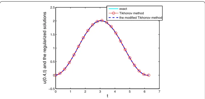
Figure compares the stability of the regularized solution computed by the classic Tikhonov method and the modified Tikhonov method at fixed pointx= . withε= .. The relative root mean square errors for them aree(u) = . ande(u) = .,
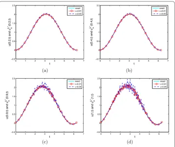
Figure 2 Comparison of the exact solution with the modified Tikhonov regularized solution. (a)x= 0.2,(b)x= 0.4,(c)x= 0.9,(d)x= 1.
Table 1 The relative root mean square errors withε= 0.01 andε= 0.05 for Example 1
x 0.2 0.4 0.6 0.8 0.9 1
e0.01(u) 0.0051 0.0059 0.0095 0.0198 0.0300 0.0460 e0.05(u) 0.0245 0.0254 0.0299 0.0457 0.0627 0.0899
spectively. For these two methods, there is almost no difference in the numerical results. However, in theoretical analysis, it is much easier to obtain the explicit error estimate for the modified Tikhonov method than to do it for the classic Tikhonov method.
Figure gives the comparison of the exact solution and its approximations with different noise. Since the exact solutionu(x,t) is a periodic function with variablet, the approxi-mate solution converges to the exact solution everywhere. We see that the approximations are acceptable for both interior and boundary temperature, and the numerical results are stable with the increase of noisy levels.
Table shows the relative root mean square errors for different x withε= . and ε= ., respectively. From this table, it is easy to see that the smaller thexthe better the computed approximation. This is consistent with the theoretical result (.).
In the next example, we will show the case in which the exact solution is not given.
Example The solution itself satisfies the following equations:
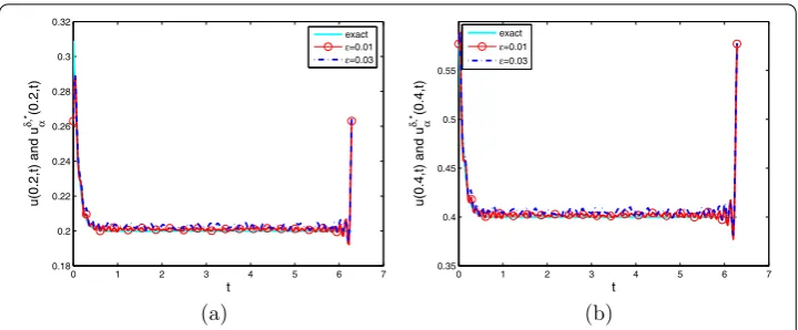
Figure 3 Comparison of the exact solution with the modified Tikhonov regularized solution. (a)x= 0.2,(b)x= 0.4.
u(,t) = , ≤t≤π, (.)
u(,t) =H(t), ≤t≤π,
whereH(t) is the Heaviside function. We use the method of the fundamental solution [] to solve the forward problem and obtaing(t) =ux(,t). The boundary datag(t) is disturbed
by a random error, and the modified Tikhonov method is used to stabilize this inverse heat conduction problem.
For this example, we can calculate by Matlab that E= ., and the regularization parameterα= ., . forε= ., ., respectively.
In Figure , we see that the regularized solution is drastically oscillatory att= π, while the numerical result is acceptable for other points. The reason for this phenomenon is that the solutionu(x,t) is not periodic to variablet, and thus the Fourier series (.) does not converge at the endpoint.
6 Conclusion
In this paper, the inverse heat conduction problem with only boundary value in a bounded domain has been investigated. The conditional stability is given. We propose a modified Tikhonov regularization method for obtaining a regularized solution. Based on ana priori
assumption for the exact solution, the order optimal error estimate is obtained with a suitable choice of regularization parameter. Numerical examples show that our proposed method is effective and stable.
Competing interests
The authors declare that they have no competing interests.
Authors’ contributions
All authors read and approved the final manuscript.
Author details
1College of Science, Henan University of Technology, Zhengzhou, 450001, P.R. China.2School of Mathematics and
Information Science, Yantai University, Yantai, Shandong 264005, P.R. China.
Acknowledgements
Received: 11 February 2016 Accepted: 6 May 2016 References
1. Dorroh, JR, Ru, XP: The application of the method of quasi-reversibility to the sideways heat equation. J. Math. Anal. Appl.236(2), 503-519 (1999)
2. Hadamard, J: Lectures on the Cauchy Problems in Linear Partial Differential Equations. Yale University Press, New Haven (1923)
3. Eldén, L: Approximations for a Cauchy problem for the heat equation. Inverse Probl.3, 263-273 (1987)
4. Hào, DN, Reinhardt, HJ, Schneider, A: Numerical solution to a sideways parabolic equation. Int. J. Numer. Methods Eng.50(5), 1253-1267 (2001)
5. Engl, HW, Hanke, M, Neubauer, A: Regularization of Inverse Problems. Kluwer Academic, Boston (1996)
6. Eldén, L, Berntsson, F, Regi ´nska, T: Wavelet and Fourier methods for solving the sideways heat equation. SIAM J. Sci. Comput.21(6), 2187-2205 (2000)
7. Regi ´nska, T, Eldén, L: Solving the sideways heat equation by a wavelet-Galerkin method. Inverse Probl.13(4), 1093-1106 (1997)
8. Regi ´nska, T, Eldén, L: Stability and convergence of wavelet-Galerkin method for the sideways heat equation. J. Inverse Ill-Posed Probl.8, 31-49 (2000)
9. Cheng, W, Fu, CL: Solving the axisymmetric inverse heat conduction problem by a wavelet dual least squares method. Bound. Value Probl.2009, Article ID 260941 (2009)
10. Carasso, A: Determining surface temperatures from interior observations. SIAM J. Appl. Math.42, 558-574 (1982) 11. Murio, DA: The Mollification Method and the Numerical Solution of Ill-Posed Problem. Wiley, New York (1993) 12. Murio, DA: Stable numerical evaluation of Grünwald-Letnikov fractional derivatives applied to a fractional IHCP.
Inverse Probl. Sci. Eng.17(2), 229-243 (2009)
13. Garshasbi, M, Dastour, H: Estimation of unknown boundary functions in an inverse heat conduction problem using a mollified marching scheme. Numer. Algorithms68(4), 769-790 (2015)
14. Hon, YC, Wei, T: The method of fundamental solutions for solving multidimensional inverse heat conduction problems. Comput. Model. Eng. Sci.7(2), 119-132 (2005)
15. Wróblewska, A, Frackowiak, A, Cialkowski, M: Regularization of the inverse heat conduction problem by the discrete Fourier transform. Inverse Probl. Sci. Eng.24(2), 195-212 (2016)
16. Wang, Y, Cheng, J, Nakagawa, J, Yamamoto, M: A numerical method for solving the inverse heat conduction problem without initial value. Inverse Probl. Sci. Eng.18(5), 655-671 (2010)
17. Ginsberg, F: On the Cauchy problem for the one-dimensional heat equation. Math. Comput.17, 257-269 (1963) 18. Liu, JC, Wei, T: A quasi-reversibility regularization method for an inverse heat conduction problem without initial data.
Appl. Math. Comput.219, 10866-10881 (2013)
19. Yang, F, Fu, CL: The method of simplified Tikhonov regularization for dealing with the inverse time-dependent heat source problem. Comput. Math. Appl.60(5), 1228-1236 (2010)
20. Cheng, W, Fu, CL, Qian, Z: A modified Tikhonov regularization method for a spherically symmetric three-dimensional inverse heat conduction problem. Math. Comput. Simul.75(3-4), 97-112 (2007)