PREDICTION OF SURFACE ROUGHNESS AND
APPLICATION OF RESPONSE SURFACE
METHODOLOGY TO DEVELOP A
MATHEMATICAL MODEL
N. Biswas
1, J. De
2, R. S. Sen
3, B. Oraon
3, G. Majumdar
3Student, Department of Mechanical Engineering, Jadavpur University, Kolkata 700032, India1 Assistant Professor, Seacom Engineering College, Howrah, India2
Professor, Department of Mechanical Engineering, Jadavpur University, Kolkata 700032, India3
Abstract: Ni-Cu-P coating was deposited on 99.99% pure Copper substrate electrolessly. The central composite design of experiment has been considered as the statistical analysis tool. The variation in surface roughness is studied by varying three parameters Ni-ion concentration, Cu-ion concentration and reducing agent concentration of the chemical bath. The surface roughness is considered as the response in student‟s t test and it has been observed that the Ni –ion source and Cu-ion source significantly influence the surface roughness at 10% level of significance. Also all the main effects (Ni-ion source, Cu-ion source, reducing ion source) and the interaction of Ni-ion and reducing agent, significantly influence the surface roughness at 20% level of significance. A mathematical model has developed considering second order response surface methodology which further considers the main effects as well as the effects of interaction and the effects of curvatures.
Keywords: Student‟s t test, Electroless Ni-Cu-P coating, RSM, CCD I. INTRODUCTION
The term “Surface Roughness” refers to the deviation or undulation of a surface from a mean level on a given length of the surface. The surface roughness of electroless Ni-Cu-P coating is a very important property, as it determines the resistance to corrosion, predicts the wear phenomenon and determines the friction properties which helps to find the micro-hardness values of the coating-substrate combinations. The electroless bath typically consists of an aqueous solution of metal ions, reducing agents, complexing agents and stabilizers operating in a special ion concentration, temperature and pH ranges [12]. The basic chemical reactions for the electroless plating are as follows [12]:
Rn+ R(n+z) + ze Mez+ + ze Me
Though copper have good mechanical properties and high thermal conductivity but oxidation and wear is a major problem in copper which can be solved by Ni-Cu-P coating without changing the bulk property of the substrate.
II. EXPERIMENTAL DETAILS
In this present work electroless Ni-Cu-P coating has been deposited on 20 × 15 × 0.1 𝑚𝑚3 99.99% pure Copper
samples by Electrolessly. The samples are cut from 99.99% pure Copper strips and first rinsed in distilled water for cleaning and then the samples are acid pickled in dilute HCL. Then again they are rinsed in distilled water. Then the samples are kept to dry. The electroless bath comprised of the following chemical as shown in table 1. The bath is alkaline.
TABLEI
DIFFERENT EXPERIMENTAL FACTORS WITH THEIR RANGES
Factors Range
NiSO4, 7H2O 23.18 – 56.82 (gm/lit) CuSO4, %H2O 0.86 – 1.54 (gm/lit) NaH2PO2, H2O 25.908 – 46.092 (gm/lit) Na3C6H5O7, 2H2O 55 (gm/lit)
CH3COONa, 3H2O 20 (gm/lit)
Temperature 85oC
After the deposition of coating for 30 mins the samples are rinsed in distilled water and then properly dried. Then The surface roughness measurements are done by TalySurf machine by Taylor Hobson Precision Instrument Surtronic 3+. Both Horizontal Magnification (around 100) and Vertical Magnification (around 10000) are done by the instrument accordingly. The surface roughness measurements are taken over a standard sample-length of 25 mm.
Fig. 1 A sample measurement of the surface profile by Talysurf instrument (without levelling)
Fig. 2 Measurement of the surface profile of the above sample by Talysurf instrument (with levelling)
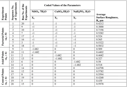
TABLEIII
AVERAGE SURFACE ROUGHESS OF THE AS-DEPOSITED SAMPLES AS FOUND IN FACTORIAL,AXIAL AND CENTRAL POINTS
III.STATISTICAL ANALYSIS
The Central Composite Design (CCD) is used for modelling a second-order response surface, A CCD consists of lk factorial or fractional factorial points, nf (usually coded ±1 rotation), 2k axial points [(±a,0,0, . . ., 0), (0,±a, 0, . . ., 0), (0, 0,±a, . . ., 0), . . ., (0, 0, . . .,±a)] and nc central points [(0, 0, 0,. . ., 0)] and central points, nc (to make CCD orthogonal or uniform precision design). The uniform precision design means that the variance of the response at origin is equal to the variance of the response at a unit distance from the origin. A uniform precision design ensures more
µm -4 -3 -2 -1 0 1 2 3 4 5
0 0.2 0.4 0.6 0.8 1 1.2 1.4 1.6 1.8 2 2.2 2.4 2.6 2.8 3 3.2 3.4 3.6 3.8 mm Length = 4 mm Pt = 3.56 µm Scale = 10 µm
µm -8 -6 -4 -2 0 2 4 6 8 10
0 0.1 0.2 0.3 0.4 0.5 0.6 0.7 0.8 0.9 1 1.1 1.2 1.3 1.4 1.5 1.6 1.7 1.8 1.9 mm Length = 2 mm Pt = 11.5 µm Scale = 20 µm
Ex p er im en t Po in ts S eq u en ce No . o f Ex p er im en ts Run No . o f th e Ex p er im en ts
Coded Values of the Parameters
Average
Surface Roughness, Ra µm
NiSO4. 7H2O CuSO4.5H2O NaH2PO2. H2O
X1 X2 X3
Fa cto ria l Po in ts (n f = 8 )
1 20 -1 -1 -1 0.4212
2 9 +1 -1 -1 0.3888
3 10 -1 +1 -1 0.7196
4 7 +1 +1 -1 0.5282
5 17 -1 -1 +1 0.524
6 16 +1 -1 +1 0.565
7 3 -1 +1 +1 0.5322
8 18 +1 +1 +1 0.5832
Ax ia l Po in ts (n a = 6 )
9 1 -1.682 0 0 0.509
10 11 +1.682 0 0 0.4402
11 2 0 -1.682 0 0.4682
12 13 0 +1.682 0 0.327
13 6 0 0 -1.682 0.58
14 4 0 0 +1.682 0.518
Ce n tr a l Po in ts (n c = 6 )
15 14 0 0 0 0.6798
16 12 0 0 0 0.5782
17 8 0 0 0 0.5594
18 19 0 0 0 0.4268
19 5 0 0 0 0.439
protection against bias in the coefficients than an orthogonal design. A CCD can be made rotatable by selecting the appropriate value of α and for a rotatable CCD, α =±4 nf.
Therefore,
0
i
=central point of the design or the basic level ith parameter =
2
m in m ax
i
i
0
i
= unit or interval of variation on the Zi axis for the ith parameter =
2
m in m ax
i
i
i
= i-th independent variable =
0 0 i i i
Zi = actual value of the i-th process parameter
Zimax = maximum actual value of the i-th process parameter
Zimin = minimum actual value of the i-th process parameter Let, k = No. of factors = 3 and l = No. of levels = 2,
nf = No. of factorial points = lk = 2 3 = 8, na = No. of axial points = 2 × k = 2 × 3 = 6 and nc = No. of central points = 6
Z = Total no. design points or total no. of observations = nf + na + nc = 8+6+6=20 Now, for Central Composite Design (CCD), the value of α = 4
48
1
.
682
f
n
In order to determine the significance of individual process parameters as well as their interactions, the following equation can be considered [14]:
Ra= β0 +β1X1 + β 2X2 + β3 X3 + β12X1X2 + β 13 X1X3 +β 23 X2X3 +β123X1X2X3 +ε Where ε represents an error component
The corresponding fitted equation can be expressed as follows [14]:
𝑅 a = E (Ra- ε) =
ˆ
0 +
ˆ
1X1 +
ˆ
2X2 +
ˆ
3X3 +
ˆ
12X1X2 +
ˆ
13 X1X3+
ˆ
23 X2X3+
ˆ
123 X1X2X3 Where β0, β1 β2, β3,. ……β123 and
ˆ
0,
ˆ
1,
ˆ
2,….,
ˆ
12,…,
ˆ
123, are the regression co-efficients.The co-efficients of the factors of the fitted equation are obtained through the Regression analysis in MINITAB Release 13.1 statistical software.
Regression Analysis equation for Ra versus X1, X2, X3, X1X2, X2X3, X3X1, X1X2X3
𝑅 = 0.519 + 0.0493𝑋𝑎 1+ 0.0274𝑋2+ 0.0492𝑋3− 0.0104𝑋1𝑋2− 0.0006𝑋2𝑋3+ 0.0284𝑋3𝑋1− 0.0170𝑋1𝑋2𝑋3
The estimated„t‟ values for particular process parameter can be obtained from the following equation:
t estimated =
ˆ
parameters
process
of
t
Coefficien
If for a particular regression coefficient, t estimated > t α, v, then the main effect or the interaction of the factors corresponding to that particular regression coefficient is significant, i.e. the factor or the interaction significantly affect the process response.
σe2 = Replication variance =
6 1 2 1 C n i c avg acti n Ra Ra= Estimate of error
Where, Raacti= Actual value of the surface roughness for the i-th central point.
Raavg= Average value of surface roughness for the central points.
n
c= No. of central points = 6 & DOF=n
c
1
= 6–1 = 5
0.51956 ) 5823 . 0 524 . 0 4268 . 0 565 . 0 597 . 0 4212 . 0 ( avg Ra Now, σe2 =
1
6
)
0039384
.
0
002025
.
0
00859329
.
0
00207025
.
0
00600625
.
0
00966289
.
0
(
= 0.006059354 Now σβ2 = σe2
/ nf Where, nf = No. of factorial points. = 8.
So, σβ2 = 0.006059354/ 8 = 0.00075741925 → σβ= 0.02752
TABLEIIIII
ESTIMATED T-VALUES OF THE PROCESS PARAMETERS AND THEIR INTERACTIONS
TABLEIVV
FONT SIZES FOR PAPERS TABULATED VALUES OF STUDENT‟S T-DISTRIBUTION
Degrees Of Freedom Level of Significance 0.1 0.2 5 t0.1;5 = 1.476 t0.2;5 = 0.92
TABLEV
FONT SIZES FOR PAPERS COMPARISON OF ESTIMATED T-VALUES OF THE COEFFICIENTS WITH THE TABULATED VALUES OF STUDENT‟S T-DISTRIBUTION
Sl No. Student’s t co-efficients Estimated t-values t0.1;5 = 1.476 t0.2;5 = 0.92
1 t1 1.7914 Significant Significant
2 t2 0.9956 Insignificant Significant
3 t3 1.7878 Significant Significant
4 t12 0.3779 Insignificant Insignificant
5 t23 0.0218 Insignificant Insignificant
6 t13 1.032 Insignificant Significant
7 t123 0.6177 Insignificant Insignificant
From the above table it can be concluded that (X1, X3) two of the main effects are significant at 10% & all the main effects (X1, X2, X3)at 20% level of significance. The interactions X13 is also significant at 20% level of significance. The other interactions are insignificant at both 10% & 20% level of significance.
IV.MATHEMATICAL MODEL FOR SECOND ORDER RESPONSE SURFACE
Response Surface Methodology (RSM) consists of statistical and mathematical techniques which are useful for developing, improving, and optimizing processes. The most extensive applications of RSM can be found in situations when several input variables potentially influence some performance measure or quality characteristic of a process. Thus performance measure or quality characteristic is called the response. This input variables are independent variables. Response Surface method develops a model that describes a continuous surface which connects the measured data taken at strategically important places in the experimental window. It also models the effects of parameters at different levels. RSM uses a least square curve-fit to develop a mathematical model tests its validity and analyze the developed model. RSM has the ability to predict, with statistical limits, the behaviour of the process at any point within the design window. The independent variables (denoted by X1, X2…Xk) are assumed to be continuous and can be controlled with negligible error. The response is postulated to be a random variable. The response is postulated to be a random variable. For three independent variables X1, X2 and X3, the response Ra can be represented as a function of X1, X2 and X3 as follows [14]:
Ra= f (X1, X2, X3) + ε If the expected response is denoted by 𝑅 a = E (Ra- ε), then the response surface is represented by
𝑅 a = f (X1, X2, X3).
A second or higher order RSM Model is necessary to approximate the surface around a curvature. In most cases, a
second order RSM model is adequate which can be represented by the following equation:
Ra=
k
i
j i j i ij k
i
k
i
k
i i i i
iX X X X
1
1 1 1
2
0
The fitted equation is represented by [14]:
𝑅 a = E (Ra- ε) =
ki
j i j i ij k
i
k
i
k
i i i i
i
X
X
X
X
1
1 1 1
2
0
ˆ
ˆ
ˆ
ˆ
=
ˆ
0 +
ˆ
1 X1 +
ˆ
2 X2 +
ˆ
3 X3+
ˆ
11X1X1+
ˆ
22 X2X2 +
ˆ
33 X3X3+
ˆ
12 X1 X2 +
ˆ
23 X2X3 +
ˆ
13 X1 X3 Where, ε = error component.Constant X1 X2 X3 X12 X23 X13 X123
σe
2 σ
β t0 t1 t2 t3 t12 t23 t13 t123
E = a mathematical expectation
The co-efficients of the fitted equations are obtained through the Response Surface Analysis in MINITAB Release 13.1 statistical software. The Second Order Response Surface Equation for Surface Roughness (Ra µm) is as follows:
R = 0.51985 + 0.04932Xa 1+ 0.02736X2+ 0.04925X3+ 0.01101X1X1− 0.00490X2X2− 0.00695X3X3
+ 0.01040X1X2+ 0.02840X1X3− 0.00055X2X3
Fig. 3 Surface Contour plots for 𝑅 = 𝑓(𝑋𝑎 1, 𝑋2)
Fig. 4 Surface Contour plots for 𝑅 = 𝑓(𝑋𝑎 2, 𝑋3)
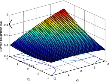
Fig. 5 Surface Contour plots for 𝑅 = 𝑓(𝑋𝑎 3, 𝑋1)
-2 -1
0 1
2
-2 -1 0 1 2 0.35 0.4 0.45 0.5 0.55 0.6 0.65
X1 X2
S
u
rf
a
c
e
R
o
u
g
h
n
e
s
s
(
R
a
)
-2 -1
0 1
2
-2 -1 0 1 2 0.35 0.4 0.45 0.5 0.55 0.6 0.65
X2 X3
S
u
rf
a
c
e
R
o
u
g
h
n
e
s
s
(
R
a
)
-2 -1
0 1
2
-2 -1 0 1 2 0.2 0.4 0.6 0.8 1
X3 X1
S
u
rf
a
c
e
R
o
u
g
h
n
e
s
s
(
R
a
The test of reliability for the predicting response surface equations has been carried out by Fisher‟s Variance Ratio known as the F-Test. The F-ratio is given by the following equation [14]:
F = σ2 res / σe2
Where, σ2
res = Residual variance =
20
1
2 N
i
esti acti
n
Z
Ra
Ra
σe2 = Replication variance =
6
1
2
1
C
n
i c
avg acti
n
Ra
Ra
n = number of coefficients in the regression equation
Raestii =estimated value of Surface Roughness for the i-th observation
The following table gives the values of σ2res , σe2 and the F-values for the for the predicting response surface equation: TABLEVV
FONT SIZES FOR PAPERS ESTIMATION OF FISHER‟S F-RATIO (FOR SURFACE ROUGHNESS)
The upper degrees of freedom (v1=Z - n) and lower degrees of freedom (v2 = nc-1) are 10 and 5 respectively. The F-value for 1% level of significance (for v1=10, v2=5) is 𝐹0.01;10,5= 10.05. The estimated F-value (1.4523) for the
prediction of response surface equation, 𝑅𝑎= f(𝑋1, 𝑋2, 𝑋3), is less than 10.05. Hence it can be concluded that the
established response surface predicting equation give a good fitting to the observed data.
V. CONCLUSION
The surface roughness is considered as the response in student‟s test and it can be concluded that the Ni –ion source and Cu-ion source significantly influence the surface roughness at 10% level of significance. Also all the main effects (Ni-ion source, Cu-ion source, reducing ion source) and the interaction of Ni-ion and reducing agent, significantly influence the surface roughness at 20% level of significance.
Fig 3-5 shows the surface plots and contour plots for𝑅 a = f(X1, X2), 𝑅 a = f(X2, X3), and 𝑅 a = f(X1, X3). From fig 3 it can be observed that, keeping X3=0, for constant values of Copper source concentration (X2), the Surface Roughness of the samples increases with the increase in Nickel source concentration (X1).For constant values of X1, the Surface Roughness of the samples increases with the increase in copper concentration (X1)
From fig 4 it can be observed that, keeping X1=0, for constant values of Copper source (X3), the Surface Roughness of the samples increases with the increase in copper concentration (X1) and then again decreases moderately. And for constant values of X2, the Surface Roughness increases upto a certain value of Copper source concentration (X2) and then again decreases moderately.
From Fig 5 it can be observed that keeping X2 = 0, for constant values of reducing agent concentration (X3), the Surface Roughness decreases moderately and then again increases moderately upto a certain value of Nickel source concentration (X1). And for constant values of X1, the Surface Roughness increases moderately upto a certain value of reducing agent concentration (X3) and then again increases.
ACKNOWLEDGMENT
The authors gratefully wish to express deep gratitude to Metrology lab, Jadavpur University, India, for providing facility to carry out the experiment.
Predicting Response
Surface Equation
Residual Variance Replication Variance Estimated F-value
Ra = f (X1, X2, X3) 0.0088
0.006059354
REFERENCES
[1] N. Parvini-Ahmadi, M. A. Khosravipour, “Electroless Deposition of Ni-Cu-P Alloy on 304 Stainless Steel by Using Thiourea and Gelatin as Additives and Investigation of Some Properties of Deposits", International Journal of ISSI, Vol.1, No. 1, pp. 29-34, 2004.
[2] Zhang Bangwei and Xie Haowen, “Effect of alloying elements on the amorphous formation and corrosion resistance of electroless Ni–P based alloys”,
Materials Science and Engineering, A281, pp. 286–291, 2000.
[3] Y. Liu and Q. Zhao, “Study of electroless Ni–Cu–P coatings and their anti-corrosion properties”, Applied Surface Science, 228, pp. 57–62, 2004.
[4] Guichang Liu, Lijun Yang, Lida Wang, Suilin Wang, Liu Chongyang and Jing Wang, “Corrosion behavior of electroless deposited Ni–Cu–P coating in flue gas condensate”, Surface & Coatings Technology, 204, pp. 3382–3386, 2010.
[5] E. Valova, J. Georgieva, S. Armyanov, I. Avramova , J. Dille, O. Kubova and M.-P. Delplancke-Ogletree, “Corrosion behavior of hybrid coatings: Electroless Ni–Cu–P and sputtered TiN”, Surface & Coatings Technology, 204, pp. 2775–2781, 2010.
[6] Q. Zhao and Y. Liu, “Electroless Ni–Cu–P–PTFE composite coatings and their anticorrosion properties”, Surface & Coatings Technology, 200, pp. 2510– 2514, 2005.
[7] Hui-Sheng Yu, Shou-Fu Luo and Yong-Rui Wang, “A comparative study on the crystallization behavior of electroless Ni–P and Ni–Cu–P deposits”, Surface and Coatings Technology, 148, pp. 143–148, 2001.
[8] E. Valovaa, J. Dilleb, S. Armyanova, J. Georgievaa, D. Tatcheva, M. Marinova, J.-L. Delplanckeb, O. Steenhautc and A. Hubinc, “Interface between electroless amorphous Ni–Cu–P coatings and Al substrate”, Surface & Coatings Technology, 190, pp. 336– 344, 2005.
[9] Q. Zhao, Y. Liu and E.W. Abel, “Effect of Cu content in electroless Ni–Cu–P–PTFE composite coatings on their anti-corrosion properties”, Materials Chemistry and Physics, 87, pp. 332–335, 2004.
[10] Liu Zhu, Laima Luo, Juan Luo, Yucheng Wu and Jian Li, “Effect of electroless plating Ni–Cu–P layer on brazability of cemented carbide to steel”, Surface & Coatings Technology, 206, pp. 2521–2524, 2012.
[11] Jen-Che Hsu and Kwang-Lung Lin, “The effect of saccharin addition on the mechanical properties and fracture behavior of electroless Ni–Cu– P deposit on Al”, Thin Solid Films, 471, pp. 186– 193, 2005.
[12] Reidel W, Electroless Ni Plating, Finishing Publications Ltd.UK, 1991.
[13] B. Oraon , G. Majumdar, B. Ghosh, “Parametric optimization and prediction of electroless Ni–B deposition”, Materials & Design, 28, pp. 2138-2147.
[14] B. Oraon, G. Majumdar, B. Ghosh, “Application of response surface method for predicting electroless nickel plating” , Materials & Design, 2006, 27, pp. 1035-1045, 2007.
[15] B. S. Choudhury, R. S. Sen, B. Oraon and G. Majumdar, “Statistical study of nickel and phosphorus contents in electroless Ni–P coatings”, Surface Engineering, 2007.
BIOGRAPHY
Dr. Rajat S. Sen is an Associate Professor in the department of Mechanical Engineering, Jadavpur University, Kolkata, India. He has vast experience in teaching and research. His current area in research includes Surface Coating, Quality Optimization, Modeling and Simulation of Production Processes. He has published a number of journal paper of national and international repute. He is presently guiding a number of research scholars in M-Tech/PhD.
Professor Buddhadeb Oraon is a Professor in the department of Mechanical Engineering, Jadavpur University, Kolkata, India. He has one year experience in reputed Industry and vast experience in teaching and research. His current area of research includes Material Science and Process Optimization.
PHOTOGRAPH
PHOTOGRAPH
Nisantka Biswas is a post graduate student in the Department of Mechanical Engineering, Jadavpur University, Kolkata, India. Her Master degree thesis is in the area of surface coating and simulation of processes.
Jhumpa De is an Assistant Professor in the Department of Mechanical Engineering, Seacom Engineering College, Howrah, India. She has four years of experience in teaching. Her current area of research includes Surface Coating, Modeling and Simulation of Processes. Jhumpa De is the corresponding author and can be contacted at :