Variable Step size LMS Algorithm Based on Discrete Cosine Transform for Voice Signal Denoising

2019 International Conference on Artificial Intelligence, Control and Automation Engineering (AICAE 2019) ISBN: 978-1-60595-643-5

Variable Step-size LMS Algorithm Based on Discrete Cosine Transform

for Voice Signal Denoising

Zhuo CHEN

Xinyang Agriculture and Forestry University, Xinyang, China

Keywords: Adaptive noise cancellation, Voice signal denoising, Discrete cosine transform, Variable step size, LMS algorithm.

Abstract. Starting from the characteristic of voice signal itself, a new variable step-size LMS algorithm based on DCT is proposed in order to improve the comprehensive performance in adaptive noise cancellation, which combines the merits of normalized DCT-LMS algorithm and variable step-size LMS algorithm, and give full play to the decorrelation capability of DCT and rapid convergence effect of variable step-size algorithm. The c simulation results show that the new algorithm has faster convergence rate and smaller steady state error compared with traditional LMS and NLMS algorithm, however, the computational complexity is comparable to NLMS algorithm at the same time.

Introduction

With the rapid development of communication technology, people's demand for quality of voice signal is growing daily, As a specific branch of adaptive signal processing, Adaptive noise cancellation technology(ANC) [1,2]can extract required signal from the loud background noise. The theoretical framework of ANC was first presented by Widrow and Hoff in 1967, now it has been applied in a great many areas such as voice signal denoising, interference cancellation in biomedical detection and echo cancellation in communication lines.

Theory of Adaptive Noise Cancellation

The original signal port receives the signals n( )from signal source which is corrupted by the noise

( )

g n from noise source at the same time, the reference input port receives the noiseX n( )which is correlated with the noiseg n( )in some way, but uncorrelated with the signals n( ). According to correlation of noise itself and independence between signals, if subtracting the filter output signal

( )

y n from the noiseg n( )and making them approaching gradually, in ideal case, the error signale n( )

can be regarded as the optimum estimation of the useful signals n( ).

Traditional LMS Algorithm

FIR filter is chosen to do the simulations, the reference input vector and the weight vector of the adaptive filter can be defined as





( ) ( ), ( 1),..., ( 1) T X n  x n x n x n m 





( ) ( ), ( ),..., _m ( )T W n  w n w n w _ n

( )

y n _{is the filter output vector,} mis the tap number, the reference input signalX n( )and the original signald n( )is real signal.

Classical LMS Algorithm

(1) Initialization: W n( )can be determined by the prior knowledge, otherwiseW(0)0

(2) If n0,1...calculate

Filter output: 1 0 ( ) ( ) ( ) ( ) ( ) ( ) ( ) m T T k k

y n w n x n k X n W n W n X n 







Error estimation: ( )e n d n( )y n( )

Update weights: W n(  1) W n( ) 2 e n X n( ) ( )

 is step-size factor for controlling convergence rate and stability, the biggeris, the shorter adaptive time becomes, but it will cause bigger misadjustment. Whenis bigger than1/_max, the system will diverge; on the contrary, the smalleris, the smaller misadjustment becomes, and the system can keep steady except for longer time. So it should be controlled in the range0  1/_max,

max

 is the largest eigenvalue of the correlation matrix.

NLMS Algorithm

(1) Initialization: W n( )can be determined by the prior knowledge, otherwiseW(0)0

(2) If n0,1...calculate

Filter output: 1 0 ( ) ( ) ( ) ( ) ( ) ( ) ( ) m T T k k

y n w n x n k X n W n W n X n 







Error estimation: ( )e n d n( )y n( )

Step-size factor: 0

0

, 0 2 ( ) ( )

T

X n X n 

  

Update weights: 2 0

( 1) ( ) ( ) ( )

( ) ( )

T

W n W n e n X n

X n X n  

  



0

 _{is a constant,}  is defined as a small value number in order to avoid the big step size when ( ) ( )

T

X n X n is very small. NLMS algorithm can reduce the dependency of convergence rate on input signal’s power estimation, so that makes it faster.

DCT-LMS Algorithm

(1) Initialization: W n( )can be determined by the prior knowledge, otherwiseW(0)0

(2) If n0,1...calculate

Discrete Cosine Transform:

1

, 0 0,1..., 1

( , )

2 (2 1)

cos , 0 1 0 j m 1

2

DCT

i j m

m

T i j

j i i m m m   _{  }      _{     } 

且

且

( ) _DCT ( ) P n T X n

2 2 2

( ) ( 1) (1 ) ( )

i i

P n P n P ni

Filter output: y n( )WT( ) ( )n P n P n W nT( ) ( )

Error estimation: ( )e n d n( )P n W nT( ) ( )

Update weights: W n(  1) W n( ) 2 e n( )2( ) ( )n P n

DCT

T is the transformation matrix of DCT,  is a small value number in the range0  0.1,

2

( )n



 is a diagonal matrix whose element values are reciprocals ofP n( )’s element power values

added on,is a contant which can keep the second part of the equation in a proper range. As for real voice signal, its energy is mainly concentrated in the low-frequency part, so DCT can be used to weaken the coefficient whose noise energy is concentrated to reduce the eigenvalue distribution of the autocorrelation matrix of the input signal to improve the convergence rate because of its good Energy compression property and decorrelation capability.

Variable Step-size LMS Algorithm Based on DCT

A normalized DCT-LMS algorithm is proposed in literature cite[5], it has good convergence rate and stable convergence performance, however, the initial mean square error is big, besides its convergence rate is worse than that of RLS algorithm. A improved variable step-size LMS algorithm based on Sigmoid function is proposed in literature cite[6], it controls the step size by using of the error correlation valuee n e n( ) ( 1),and makes it correlated with useful signal but uncorrelated with noise signal, so that reduce the sensitivity to noise and keep the computational complexity at a low level. According to the issues above, a new variable step-size LMS algorithm based on DCT(VS-DCT-LMS) is proposed which combines both of their merits.

(1) Initialization: W n( )can be determined by the prior knowledge, otherwiseW(0)0

(2) If n0,1...calculate

Discrete Cosine Transform:

1

, 0 0,1..., 1

( , )

2 (2 1)

cos , 0 1 0 j m 1

2

DCT

i j m

m

T i j

j i

i m

m m



 _{  }

  



 _{     }



且

且

( ) _DCT ( ) P n T X n

2 2 2

( ) ( 1) (1 ) ( )

i i

P n P n P ni

     i0,1,...,m1 Filter output: y n( )WT( ) ( )n P n P n W nT( ) ( )

Error estimation: ( )e n d n( )P n W nT( ) ( )

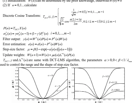
Step-size factor:   (1 exp(  e n e n( ) ( 1) ))

Update weights: W n(  1) W n( )e n( ) 2( ) ( )n P n

DCT

T , and2( )n are same with DCT-LMS algorithm, the parameters  0, 0  1/_maxare used to control the range and the shape of step-size factor.

Figure 1. Relation curve between( )n ande n( ). Figure 2. Relation curve between( )n ande n( ).

= different

 

From Figure 1 and Figure 2, it is clear to see that the absolute value ofe n( )is big in the initial stages, so is( )n _{, and the convergence rate is fast. When the algorithm reaches steady state,} e n( )

and( )n both get the minima. If keeping one parameter and changing the other on the premise of satisfying convergence requirements, the bigger the changed one is, the faster convergence rate becomes.

Simulation Results and Performance Comparison

In order to test the filtering performance of each algorithm, a Matlab simulation is performed on a 4-order FIR filter, the Gause white noise which has a zero mean is added into the useful signal

( ) sin(0.01* * )

s n  pi n , the initial signal to noise ratio(SNR) is set to 3dB, so the original signal

( )

d n is composed of sinusoidal signals n( )and the Gause white noise. Parameters of each algorithm are set as follows:

LMS algorithm: 0.005

NLMS algorithm: 0.01, 0.001

DCT-LMS algorithm: 0.5, 0.99,0.01

VS-DCT-LMS algorithm: 20, 0.25, 0.99

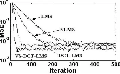
100 independent experiments are done to get an average result. The learning curves are shown in Figure 3. Obviously, the convergence rate of DCT-LMS algorithm and VS-DCT-LMS algorithm is faster than that of LMS algorithm due to the decorrelation capability of DCT. NLMS algorithm overcomes the dependency of convergence rate on input signal’s power estimation and keeps the feature of simple implementation, but its steady state error is big, there is still some room for the convergence rate to be improved. By using of new step-size factor, VS-DCT-LMS improves convergence performance and meanwhile keeps the low steady state error, so its comprehensive performance is better than the others.

Figure 3. Learning curves of 4 adaptive algorithms.

Figure 4. Waveforms and frequency spectrum of useful signal s n( ) and original signal d n( ).

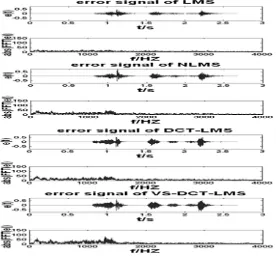
Figure 5. Waveforms and frequency spectrum of error signal e n( ).

Conclusion

The comprehensive performance of several algorithms in adaptive noise cancellation are compared with each other in this paper. A new variable step-size LMS algorithm based on DCT is proposed which combines both of their merits. Through the voice signal denoising simulation, results show that the new algorithm has the best filter effect and adaptability under low SNR.

References

[1] Hongyu Chen. Research of adaptive filtering algorithm and application in VoIP system[D]. Zhejiang University of Technology, 2017.

[2] Xinyin Yu. An adaptive multi-channel anti-noise system[J].Journal of Changchun University of Technology, 2015,(5): 552-555.

[3] Huang B, Xiao Y, Ma Y, et al. A simplified variable step-size LMS algorithm for Fourier analysis and its statistical properties[J].Signal Processing, 2015,117:69-81.

[5] Xiaoling Ning, Zhong Liu, et al.Fast convergence transform domain adaptive filter algorithm[J]. Journal of Electronic Measurement and Instrumentation, 2011, 25(3):240-245.