Feature Selection in Computational Biology

(1)

Feature Selection in Computational Biology

Dimitrios Athanasakis

A dissertation submitted in partial fulfillment of the requirements for the degree of

Doctor of Engineering of the

University of London.

Department of Computer Science University College London

(2)

I, Dimitrios Athanasakis, confirm that the work presented in this thesis is my own. Where information has been derived from other sources, I confirm that this has been indicated in the

(3)

Abstract

This thesis concerns feature selection, with a particular emphasis on the computational biology domain and the possibility of non-linear interaction between features. Towards this it establishes a two-step approach, where the first step is feature selection, followed by the learning of a kernel machine in this reduced representation.

Optimization of kernel target alignment is proposed as a model selection criterion and its properties are established for a number of feature selection algorithms, including some novel variants of stability selection. The thesis further studies greedy and stochastic approaches for optimizing alignment, propos-ing a fast stochastic method with substantial probabilistic guarantees. The proposed stochastic method compares favorably to its deterministic counterparts in terms of computational complexity and resulting accuracy.

The characteristics of this stochastic proposal in terms of computational complexity and applicabil-ity to multi-class problems make it invaluable to a deep learning architecture which we propose. Very encouraging results of this architecture in a recent challenge dataset further justify this approach, with good further results on a signal peptide cleavage prediction task.

These proposals are evaluated in terms of generalization accuracy, interpretability and numerical stability of the models, and speed on a number of real datasets arising from infectious disease bioinfor-matics, with encouraging results.

(4)

Acknowledgements

Some of the few things surpassing professor John Shawe-Taylor’s depth and breadth of knowledge on the subject of machine learning is his patience and encouragement towards students. My time working with John has been a privilege. I also need to thank my second supervisor, dr Delmiro Fernandez-Reyes for providing his support whenever it was asked for, during numerous occasions throughout my degree.

The people who have spent time reviewing my work as part of the thesis comittee have been pivotal in shaping the thesis. These include Mark Herbster, Juho Rousu, and Arthur Gretton. Their collective input has had great impact on the thesis.

The division of parasitology at the National Institute for Medical Research and the computer science department at UCL have been great places to work. They have my thanks for being excellent sources of interesting new problems and applications, and for giving me some of the smartest friends I’ve met to this day.

Finally, I would like to thank my family for always being there. This thesis is the result of my parents’ encouragement to work on whatever I find fulfilling. Thank you.

(5)

List of Figures

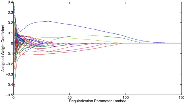
2.1 regularization path for lasso on TB dataset. The TB dataset comprises 523 features. Here, each line represents the computed weight-coefficients for each variable at varying levels of regularization. It can be seen that for increasing amounts of regularization, controlled by the parameterλ, the 1-norm of the weightwdecreases, resulting in models that rely on fewer variables. Theλparameter essentially controls the exchange between sparsity and goodness of fit for the Lasso problem. . . 25 2.2 Examples of selected features over 30 cross-validation folds for a toy 20-dimensional

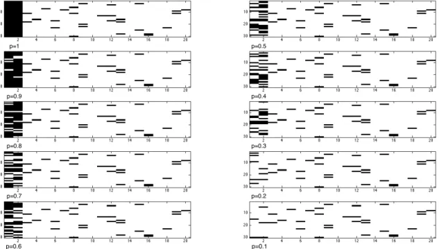
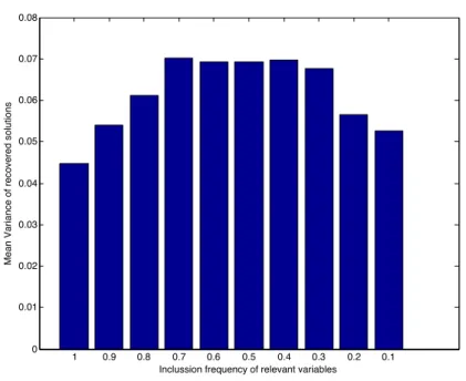
dataset. Black bars indicate that the the feature was selected for that fold(features:left-to-right, folds: top-to-bottom). We consider the first two features to be relevant, and selected with varying probability between 1 and 0.1. The remaining, features are selected uniformly at random with a probability of 0.05. . . 28 2.3 Example Mean Variance for different inclusion probabilities of the relevant features in

the scenarios of figure 2.2. This figure illustrates that only estimating the variance of a feature can be misleading. In this example, selecting the two relevant features with probability 0.9 appears to have larger mean variance than selecting them with probability 0.1. . . 29 2.4 Plot for the log likelihood corresponding to the different selection probabilities of the

relevant features. The correspondence between log likelihood and the high selection rate of the relevant components is substantially improved. For selection probabilities 0.2 and 0.1 the log likelihood is positive, as we are estimating an upper bound of the true probability. . . 29

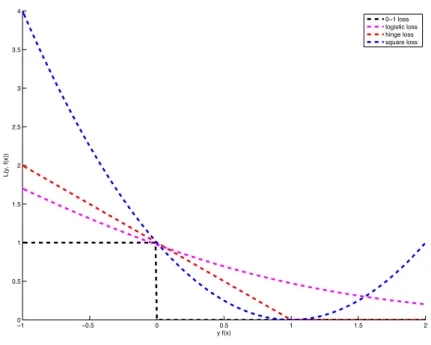
3.1 Dependence of target alignment on theσparameter of the gaussian kernel. For increasing number of irrelevant features, smaller values ofσtend to produce higher alignment. This appears to stem from increasing the effective dimensionality, and has been also observed in ([SFG+_{09], sec. 5).} _{. . . .} ₃₄ 3.2 Different loss functions for classification. The lasso minimises the square loss (blue).

The 0-1 loss function(black), which is directly related to accuracy, is NP-hard to opti-mise. Two loss functions commonly applied to classification problems are the logistic loss (magenta), and the hinge loss(red), that act as proxies for the 0-1 loss. . . 35

(8)

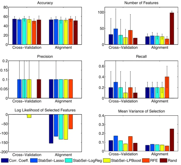
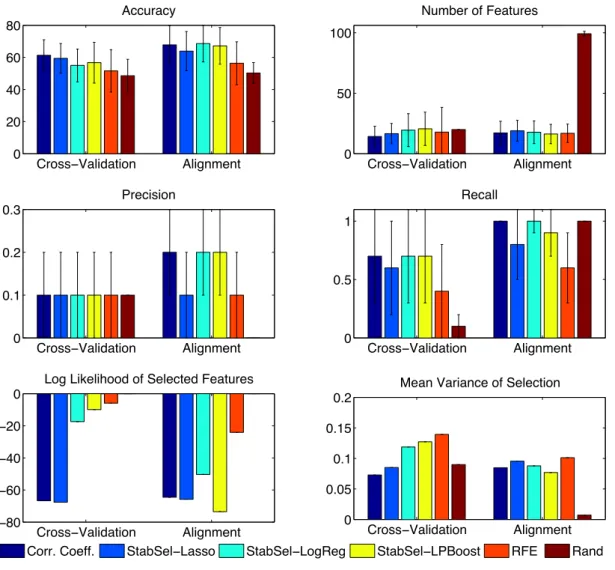
3.3 Results for the fake class dataset. Rand selects a random 10% of the variables in the cross-validation setting, or the subset of a random ordering of variables which maximises alignment in the alignment case. . . 39 3.4 Results for the Linear Zhang with Feature Noise. Rand selects a random 10% of the

variables in the cross-validation setting, or the subset of a random ordering of variables which maximises alignment in the alignment case. . . 40

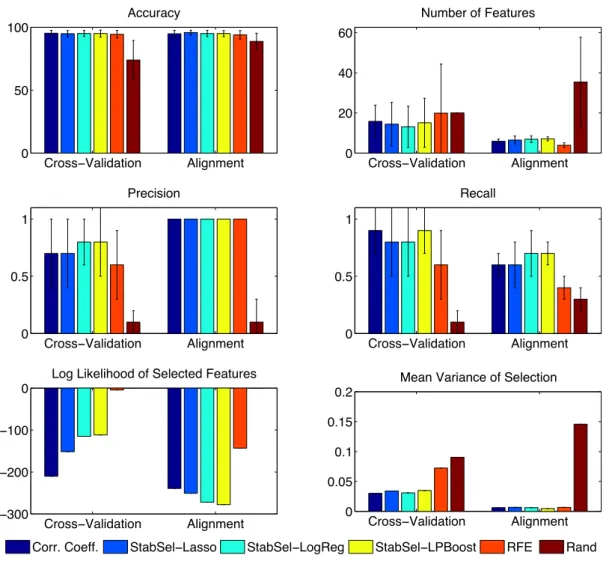
3.5 Results for the linear Zhang dataset with sample noise. Rand selects a random 10% of the variables in the cross-validation setting, or the subset of a random ordering of variables which maximises alignment in the alignment case. . . 41 3.6 Results for the linear Weston dataset. Rand selects a random 10% of the variables in the

cross-validation setting, or the subset of a random ordering of variables which maximises alignment in the alignment case. . . 42

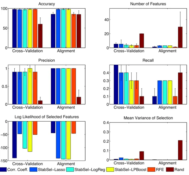
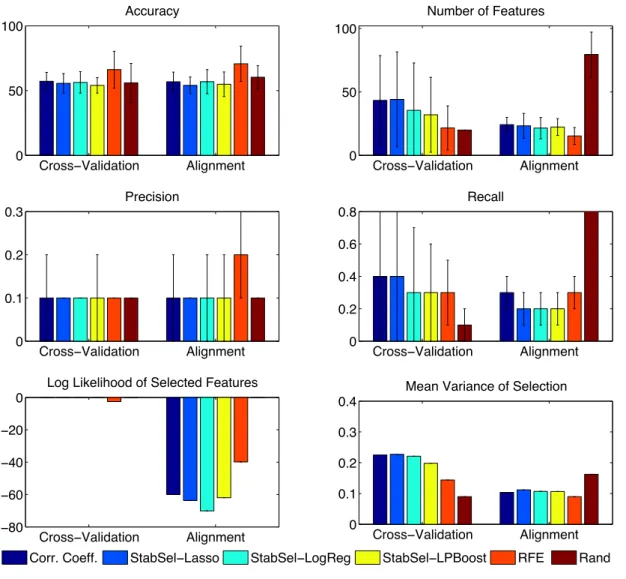
3.7 Results for the non-linear Weston dataset. Rand selects a random 10% of the variables in the cross-validation setting, or the subset of a random ordering of variables which maximises alignment in the alignment case. . . 43 3.8 Results for the XOR dataset. Rand selects a random 10% of the variables in the

cross-validation setting, or the subset of a random ordering of variables which maximises alignment in the alignment case. . . 44

3.9 Results for the first TB task. Rand selects a random 10% of the variables in the cross-validation setting, or the subset of a random ordering of variables which maximises alignment in the alignment case. . . 45

3.10 Results for the second TB task. Rand selects a random 10% of the variables in the cross-validation setting, or the subset of a random ordering of variables which maximises alignment in the alignment case. . . 46

3.11 Accuracy results for the third TB task. Rand selects a random 10% of the variables in the cross-validation setting, or the subset of a random ordering of variables which maximises alignment in the alignment case. . . 46

3.12 Results for the fourth TB task. Rand selects a random 10% of the variables in the cross-validation setting, or the subset of a random ordering of variables which maximises alignment in the alignment case. . . 47

3.13 Results for the TB micro-array task. Rand selects a random 10% of the variables in the cross-validation setting, or the subset of a random ordering of variables which maximises alignment in the alignment case. . . 48

(9)

List of Figures 9 4.1 Mean alignment as a function of sample size. For each sample size the mean alignment

is computed on 500 bootstraps of the data. Black line corresponds to a a random 25-dimensional multivariate gaussian. Red line depicts the mean alignment of 2 relevant variables generated according to the [WMC+_{00], and 23 gaussian probes. Green depicts} the alignment for only the two relevant features. The influence of self-interaction terms (the diagonal termscxiicyii) decreases for larger sample sizes, leading to the displayed

drop here. . . 52

4.2 Scatter plot of the resulting alignment over random splits of variables for an XOR dataset with the additional inclussion of a varying number of irrelevant variables (blue n=5, green n=10, red n= 15, light blue n= 20, magenta n = 25, bootstrap size = 100 samples). Over the different number of dimensions, a common pattern emerges: Samples concen-trated over the lower left corner correspond to estimates in which each random split of the variables contains a single relevant feature, resulting in lower alignment for both splits. The bottom-right and top-left corners contain cases where one split contains both of the relevant variables, resulting in a visible hike in alignment for that split. It is also particularly instructive to notice that for samples corresponding to higher signal-to-noise ratios, the variance of the resulting alignment seems to be much higher, further justifying subsampling. . . 54

4.3 200-dimensional XOR classification problem. The expected contribution of the two rel-evant features is in red. It can be seen that as more of the noise features are removed in latter iterations of the method, the expected contribution of the two relevant variables rises substantially, in contrast to the contribution of the other features. . . 57

4.4 Results for the fake class dataset. . . 62

4.5 Results for the linear Zhang with feature noise dataset. . . 63

4.6 Results for the linear Zhang with sample noise dataset . . . 64

4.7 Results for the linear Weston dataset. . . 64

4.8 Results for the non linear Weston dataset. . . 65

4.9 Results for the XOR dataset. . . 66

4.10 Results for the first TB task. . . 67

4.11 Results for the second TB task. . . 68

4.12 Results for the third TB task. . . 68

4.13 Results for the fourth TB task. . . 69

4.14 Results for the TB Micro-Array task. . . 69

5.1 Overall architecture; randSel is applied on the features learned by sparse filtering, pro-ducing a number of nonlinear combinations of learned features of increasing granularity. A number of kernels is defined on these nonlinear combinations of features, and multiple kernel learning is used for the overall prediction. . . 76

(10)

5.2 How the learned representation is generated. The amino-acid sequence is broken into smaller windows. Each amino-acid in the window is represented by its 54 distinct physic-ochemical properties. Sparse filtering is used to learn a representation for this encoding. . 80 5.3 Accuracy of different feature selection and representation approaches on the signal

pep-tide dataset. All feature selection approaches that operate on the learned representation clearly outperform the original features. Methods employing a single kernel for pre-diction result in similar accuracy. Combining randSel with MKL outperforms all other approaches. . . 82 5.4 Substantial differences in correlation between full dataset (top row) and the support

vec-tors (bottom row). This is largely due to the support vecvec-tors comprising of more atypical examples, for which the constraint of the SVM optimization problem is active. It is not visually obvious, but the two rows are very correlated, however some ordering informa-tion, which is important for feature selecinforma-tion, is lost in the active set. This means that while the ranking the features by correlation to the target output is largely similar be-tween the active set and the entire set of variables, the differences in rank are substantial enough to affect the behavior of RFE. . . 82

(11)

List of Tables

3.1 Class proportions for synthetic data. . . 38 3.2 Fold Decrease for the time requirements of different methods when using alignment

(12)

Introduction

We present a family of two-stage techniques for kernel machines. The first stage of these techniques is a feature selection method in order to reduce the number of variables while the second stage is fitting a kernel machine on this lower- dimensional dataset. Given the potential benefits of a reduced representa-tion it is not surprising that a rich variety of methods have been proposed in order to achieve this. Such algorithms are routinely used in order to alleviate problems such as the so-called curse of dimensionality and reduce generalisation error. Another common use for these methods is in reducing the storage and processing requirements for large datasets. However, the most important property as far as the field com-putational biology is concerned may be that of parsimony. Models relying on fewer variables are easier to explain and have the potential to accelerate experimental validation by providing valuable insight into the importance and role of the variables. Considering their potential applications we enumerate four highly desirable properties for the ideal feature selection algorithm:

1. Low generalization error. Feature selection should improve generalization performance, or at the very least not deteriorate the error rate as compared to learning on the full set of features.

2. Parsimony. The resulting models should use the smallest possible number of features. Models relying on fewer variables are easier to study. This can be viewed as a form of Occam’s razor whereby hypotheses that rely on fewer variables are preferred.

3. Selection Consistency. Here selection consistency means that the variables selected should not radically change for small perturbations in the data. This is a key property in computational biology wheredirtydata such as noisy outputs or labels are not uncommon.

4. Scalablility. The size of datasets is increasing at a much faster rate than speed increases in com-modity hardware can cope with. Given this simple fact, computationally efficient algorithms and methods which can be parallelized are advantageous.

1.1

Background

It is not uncommon to encounter features that exhibit a high degree of redundancy in practice. In such cases the SVM classifier tends to assign similar weights to features that exhibit a high degree of similarity between them. It is also possible however to have a large number of variables that appear to be irrelevant

(13)

1.1. Background 13 to the target concept lead to deteriorating generalization. In both of these cases it is possible for a benign collusion between feature selection mechanisms and SVMs to yield many of the benefits previously listed above. For this to occur, an effective feature selection method is expected to find a small and informative set of relevant features as well as identify features that are redundant or irrelevant to the target concept. An attempt to formalize the notions of feature relevance follows.

The following section summarizes work and definitions in [GGNZ06], where the authors attempt to produce formal mathematical definitions of the notions of feature relevance.

Making the assumption that the dependency between input patternsXand desired outputsYis gov-erned by the joint distributionP(X,Y) =P(Y|X)P(X)we introduce the following auxiliary notations. LetVbe some subset ofX,X−i bet the subset ofXexcluding featurexiandV−i be a subset ofX−i.

Those are used to make the following definitions of variable relevance or irrelevance.

1.1.0.1

Surely Irrelevant Features

A featureXiis surely irrelevant iff for all subset of featuresV−iincludingX−iwe have:

P(Xi,Y|V−i) =P(Xi|V−i)P(Y|V−i)

This definition can be extended through the use of the Kullback-Leibler divergence between P(Xi,Y|V−i)andP(Y|V−i)giving rise to the following measure of conditional mutual information,

M I(Xi,Y|V−i): M I(Xi,Y|V−i) = X {Xi,Y} P(Xi,Y|V−i) log P(Xi,Y|V−i) P(Xi|V−i)P(Y|V−i)

The above sum runs over all possible values of the random variablesXi andY. The conditional

mutual information can be used to derive a score that encapsulates the relevance of a feature Xi by

summarizing over all the values ofV−i. For the relevance of featureXi, givenY, we obtain the expected

mutual information as:

EM I(Xi,Y) =

X

V−i

P(V−i)M I(Xi,Y|V−i)

Using this quantity we can proceed to the following definitions.

1.1.0.2

Approximately Irrelevant Features

A featureXiis approximately irrelevant with level of approximation >0, iff for all subsets of features

V−iincludingX−i,

EM I(Xi,Y)≤

1.1.0.3

Surely Sufficient Feature Subsests

We have provided a definition of feature relevance. However even relevant features may be redundant. Hence, merely ranking features by their relevance is not sufficient in order to extract a minimum subset of features that produce optimal predictions. We introduce the additional notationV¯ for the subset that complements a set of featuresVinX: X= [V,V¯]. Using this we obtain that a subsetVof features is surely sufficient iff, for all assignments of values to its complementary subsetV¯

(14)

P(Y|V) =P(Y|X)

Similarly to the definition of feature relevance, we can extend this through the use of mutual infor-mation, defining a new quantity,DM I(V):

DM I(V) = X

{u,u,¯y}

P(X= [v,¯v],Y=y) logP(Y=y|X= [v,¯v])

P(Y=y|V=v)

The above quantity, which was introduced in [KS96] is the expected value over P(X) of the Kullback-Liebler divergenvence betweenP(Y|X)andP(Y|V). It can be verified that :

DM I(V) =M I(X,Y)−M I(V,Y)

1.1.0.4

Approximately sufficient feature set

Again in similarity with the previous definitions of approximate feature relevance, we have that a subset Vof features if approximately sufficient with level of approximation≥0, iff

DM I(V)≤

In the case that= 0the subsetVis calledalmost surely sufficient.

1.1.0.5

Minimal Approximately Sufficient Feature Subset

Finally a subsetVof features is minimal approximately sufficient, with level of approximation ≥ 0

iff it is-sufficient and other-sufficient subsets of smaller size do not exist. From this definition it fol-lows that a minimal approximately sufficient subset is a (possibly non-unique) solution to the following optimization problem:

minVk|V||0, s.t.DM I(V)≤

Where||V||0 is the zero norm, which equals the number of selected variables. These definitions underpin the fact that there is no one-size-fits all approach to feature selection, as objectives can vary substantially.

1.2

Approaches to feature selection

Finding the minimal approximately sufficient feature set is a NP-hard problem. Naive attempts to com-putationally identify an optimal combination of features by exhaustive search are infeasible, even for a relatively small number of variables. Practical feature selection algorithms address this limitation by using a number of proxy criteria related to the selection problem. Depending on the core criterion, three principal selection approaches can be identified:

• Filter Methods employ simple heuristics or statistical tests for evaluating the importance of a feature.

(15)

1.2. Approaches to feature selection 15 • Wrapper Methods, in contrast to filter methods tend to refine an initial solution by relying on performance bounds or empirical estimates that encapsulate the impact that removing a feature, or number of features would have to the solution of the problem.

• Embedded Methods, where feature selection is embedded as part of the learning algorithm, typi-cally by usingL1-norm minimization or similar approaches.

1.2.1

Filters

Filter methods provide a simple and fast approach to filter selection. Typically, filters rely on statistical criteria which act as a proxy for the underlying modelling problem. A typical example of this approach would be a filter that employs correlation coefficients. Making the assumption that informative features are highly correlated with the classification target, it ranks features by the magnitude of their correlation. Variables that do not exhibit a user-specified degree of correlation are filtered out of the dataset, resulting in a simple and efficient filtering method .

This simple, and efficient approach has been successfully employed in a large variety of problems. However, there are drawbacks to using correlation coefficients. First, correlation coefficients make the assumption that the underlying relation is linear. While this assumption applies to a certain degree in numerous problem domains, it is a clear limit to the scope of its application. Furthermore, correlation coefficients fail to encapsulate interactions between variables. The relief algorithm [KR92] is a multi-variate filter method which addresses some of the shortcomings of correlation coefficients. The relief method uses ak-nearest-neighbor derived criterion.At each iteration, the algorithm cycles through the samples, estimating the relevance as a function of the nearest within-class and out-of-class samples. This is achieved through comparing the distance of the ith sample to its nearest hits (closest, within class neighbors) and nearest misses (closest out-of-class neighbors), with and without the inclussion of a feature.

In recent years, information-theoretic approaches to filtering have seen substantial growth. Numer-ous methods using mutual information as an indicator of statistical dependence have been proposed, with encouraging results on real world data [ZH02]. [Bro09],[BPZL12] propose the conditional likelihood of the training labels as a unifying theme for information theoretic approaches, viewing such filters as belonging to a spectrum of approximate maximizers of the conditional likelihood and differentiated by their implicit statistical assumptions.

Another line of inquiry relies on the estimation of cross-covariance between kernels defined on the input and output data [GBSS05], which proposes the Hilbert-Schmidt Independence Criterion. This prin-cipled approach benefits from sharp concentration estimates. [SBB+_{07] illustrates procedures relying} on HSIC are fairly simple to implement, and do not require user intervention in terms of regularization. Further work utilising HSIC for feature selection is found in [SSG+_{12] where a slew of connections with} existing algorithms is presented, including its similarity to Kernel Target Alignment (KTA).

(16)

1.2.2

Wrapper Methods

Wrapper methods are strongly paired to the classification problem. One of the first wrappers, specific to support vector machines (SVMs)was introduced in [WMC+00]. The approach used gradient descent optimization on a margin bound, removing the least-weighted features after each iteration. Recursive feature elimination (RFE[GWBV02]), is similar in function, removing the least weighted feature from the actual linear predictor at the end of each iteration. In the kernelized setting, RFE is significantly more demanding. Non-linear RFE quantifies the sensitivity of the learning rule to the removal of each individual feature. This means that for non-linear, high-dimensional datasets, RFE is tractable but com-putationally prohibitive as at each iteration it needs to train a support vector machine, and then estimate the sensitivity to the individual removal of the remaining features.

1.2.3

Embedded Methods

In recent years, there has been a flurry of embedded feature selection methods. Embedded methods achieve parsimony by enforcing additional constraints to the recovered solution. Lasso,[Tib96] is one of the earliest proposals in this class of algorithms. The lasso algorithm attempts to minimise the sum of the square loss of the derived predictor and a multiple of the`1-norm of the weight vectors. Setting the regularization of the weights complicates model selection. To some degree, this complication is addressed by regularization paths. A regularization path, is a piecewise linear function that associates the regularization parameter with a corresponding recovered solution to the optimization problem. The homotopy algorithm described in [OPT00], leverages regularization paths to describe an efficient algo-rithm that computes the entire space of recovered solutions with small additional computation overhead. This is further elaborated in [EHJ+_{04] in the context of the LARS algorithm, where an algorithm that} computes the regularization path in time similar to ordinary least squares is introduced.

The Lasso objective optimizes the square loss. The square loss is applicable to a wide variety of settings, including classification and regression. In classification problems the same approach, using loss functions specific to the classification setting such as the logistic loss [LLAN06],is applied. Warm-start techniques [KKB07], use a previously computed solution as the starting point for computing the solution for an updated regularization term. For the hinge loss, commonly employed by SVMs, a regularization path approach has been proposed in the case of `2-regularized SVMs [HRTZ04]. To the best of my knowledge, there is no published work detailing a regularization path approach for`1-regularized SVMs. Boosting [FS97] can also be thought of as an embedded feature selection algorithm. Boosting at-tempts to produce a strong learning rule by combining predictions produced by weak base learners. A weak learner can be thought of as a simple prediction algorithm relying on a subset of features. By limiting the number of weak learners boosting can be effectively used as a feature selection algorithm, a procedure which is illustrated in [BY06]. The most common boosting variant, adaboost [FSA99], optimizes the exponential loss. LPBoost [DBST02] is another boosting algorithm, geared towards op-timizing the hinge loss, and in the setting where a base learner corresponds to a single feature can be thought of as an`1-regularized approach to the support vector machine.

(17)

1.3. Application to biomarker discovery 17 learning. Once more, by defining low-rank kernels on small groups of features, this approach effectively performs feature selection. Some early propositions include [LCB+04] where semi-definite program-ming was used to learn the kernel matrix. Multiple refinements to this approach have been presented, including [BLJ04], where sequential minimal optimization (SMO) techniques were utilised for greater efficiency, [SRSS06] which relies on a semi-infinite linear programming formulation and [RBCG08] which presents a simple approach which is essentially based on gradient descent. More recently an approach relying on the optimization of KTA was proposed in [CMR12] which utilises existing SVM solvers.

1.2.4

Meta-Selection Approaches

The previous sections presented the three major feature selection approaches. By meta-selection strate-gies, we refer to feature selection regimes which intelligently exploit properties of these three basic feature selection approaches. Two methods that exemplify this approach are BoLasso [Bac08] and Sta-bility Selection [MB10]. Both methods rely on bootstrapped Lasso estimates, exploiting the fact that relevant variables will enter the model with substantially higher probability than those that are irrele-vant. This property suggests that with a large number of bootstrapped lasso estimates of a given sample, intersecting their supports leads to improvements in selection consistency. This simple idea is further elaborated in [MB10], where the approach is extended to a more general framework, that combines sub-sampling with sparse selection algorithms. A significant contribution of stability selection is its ability to provide probabilistic guarantees for the false discovery rate of the selected features. Examples illustrat-ing the need for meta-selection algorithms are given in [DET06] and [CT07], where the irrepresentable condition for the Lasso and related algorithms is introduced. The irrepresentable condition is violated in scenarios where the number of variables exceeds the number of samples, and a substantial degree of between-variable correlation is present leading to inconsistent selection.

1.3

Application to biomarker discovery

Biomarkersare small, statistically validated sets of variables that strongly characterize an underlying bi-ological process. High throughput bibi-ological screening methods such as micro-arrays and time-of-flight mass spectrometry capture large numbers of variables related to biological samples. Through systematic comparison to appropriately chosen reference samples it is possible to discover, and statistically validate disease specific proteome patterns. This is a process where feature selection plays a major role. Feature selection is pivotal in shifting the focus from a very large number of variables to a substantially smaller number of of features, which at this point are considered as biomarker candidates.

Feature selection is a generic methodology that needs to effectively address the already large num-ber of extant technologies in biology as well as anticipate the advent of new technologies. In so doing, these algorithms need to retain their connection to the biological context of the problem. An example of this is [AFRP+_{06] where feature selection on mass-spectrometry data from a Tuberculosis(TB) study,} resulted in the identification of novel biomarkers. The impact of accurate algorithms is not limited to just novel diagnostics. It is often the case that biomarkers can reveal a vast amount of information on the

(18)

underlying biological process, as well as providing a target for therapeutic approaches to focus on. In terms of practical considerations, feature selection algorithms need to address a series of issues. They need to be computationally efficient in order to address the ever-increasing size of the datasets. All the other desiderata also apply, in terms of consistency, parsimony and generalization. Additionally it needs to address nuances specific to biology. Principal among these is the variance samples can exhibit. It is often the case to encounter a substantial degree of variation even for replicates of the same biological sample. A further complication comes in the form of label noise,as the classes which correspond to diagnoses on the biological samples are not always accurate. Robustness towards these factors is important.

1.4

Structure of the thesis

The rest of the thesis is structured as follows.

1. Chapter 2provides the necessary background on max-margin learning and feature selection as-sumed throughout the rest of the thesis.

2. Chapter 3examines variants of stability selection better tailored towards classification and intro-duces the greedy maximization of kernel target alignment as a model selection criterion.

3. Chapter 4presents a randomized feature selection algorithm for nonlinear feature selection and provides empirical comparisons with other non-linear feature selection variants.

4. Chapter 5studies the use of feature selection on representation learning, providing very encour-aging results.

5. Chapter 6concludes the thesis by summarizing the presentation and identifying avenues for future research.

(19)

Chapter 2

Background: Enabling Technologies

This chapter establishes the background and introduces the necessary notation for the following chapters of the thesis. We begin with the introduction of linear learning. We establish some characteristics of linear classification such as margins, as well as illustrating how kernels are utilised to address the limitations of linear learning. Going back to feature selection, algorithms that exemplify the approaches mentioned in the previous chapter are presented. Finally, we introduce metrics and the experimental pipeline for evaluation of the chapters to follow.

2.1

Linear Learning

We consider the supervised learning problem of modelling the relationship between am×ninput matrix

Xand a correspondingm×n0output matrixY. The archetypical instance of such a problem is binary classification where the objective of the learning problem is to learn a functionf :x→ymapping input vectorsxto the desired outputsy. In the binary case we are presented with am×nmatrixXand a vector of outputsy∈ {+1,−1}m_{Limiting the class of discrimination functions to linear classifiers we}

wish to find a classifier :

f(x) =X

i

wixi+b=hw, xi+b (2.1)

where the weight vectorwand biasbare parameters derived by the learning algorithm.

Beneath the simplicity of the above equation lies the most fundamental problem for most machine learning applications. The problem is that in most practical settings, learning is ill-conditioned. In simple terms this can mean that the number of samples is insufficient to guarantee the discovery of an accurate prediction rule. In the presence of noise, aiming to perfectly fit the training set often leads to overfitting, whereby the prediction function accounts for noise in the training set instead of learning a meaningful representation of the underlying problem.

Simple linear algebra guarantees that with enough variables it is possible to perfectly fit any dataset. This raises the question of how to choose from competing hypotheses that ’look good’ on the data set at hand, and how well do these competing hypotheses mirror the properties of the underlying process. Reg-ularization is an answer to the first question. RegReg-ularization places additional restrictions to the weight vector, with the most common approach being to favour solutions that have small norms. Learning the-ory attempts to answer the latter question, and SVMs combine these two insights to create an effective

(20)

algorithm.

2.2

Max margin classification and support vector machines

The signed distance of a pointx from a hyperplane(w, b)ishw,xi+b. The margin is the minimum distance between the convex hulls of the negative and positive training points. We denote asx+_,_x−_, two samples belonging to margins of the positive and negative class respectively. For a weight vectorw

realising a functional margin of 1 on the positive pointx+_{and the negative point}_x−_{we have}

hw,x+i+b= 1

hw,x−i+b=−1

To compute the geometric marginγ,wmust be normalised. The geometric marginγis the func-tional margin of the resulting classifier

γ= 1 2(h w ||w||2 x+i − h w ||w||2 x−i) = 1 ||w||2 (2.2) Equation (2.2) introduces the relation between the weight vectorw and achieved marginγ. In the linearly separable case, the SVM algorithm attempts to recover the maximal margin hyperplanew

through the following optimization problem:

minimizew,b1₂||w||2

subject to yi(hw,xii+b)≥1

i= 1, ..., m

(2.3)

Introducing slack variables to the above optimization problem we can obtain the soft-margin SVM formulation [CV95] : minimizew,b,ξ1₂||w||2+CP n i=1ξi subject to yi(hw,xii+b)≥1−ξi i= 1, ..., m ξi≥0 (2.4)

In the above formulation, the regularization parameterCcontrols the balance between goodness-of-fit and the weights of the recovered solution. Considering that the slack variablesξi are equivalent

to the hinge loss functionLhinge = max(0,1−yihw, xii), equation (2.4) exemplifies an approach

we will encounter again, namely minimising a loss function under additional weight restrictions. It is important to note that for most practical scenarios, a large number of the slack variablesξwill be zero. The discovered classification rule only depends on the few samples that lie on the margin, for which the

(21)

2.3. Non-linear maps and kernels 21 inequality constraint is active and thereforeai >0. These samples are called support vectors, lending

their name to the algorithm.

An examination of the max-margin approach would be incomplete without some mention of the wealth of learning theory relating the marginγ with generalization. Indeed, a large body of work is dedicated to establishing bounds for generalization performance of support vector machines in terms of the margin distribution. In [STBWA98], it was shown that margins and the number of support vectors can be used to estimate how well the recovered classifier relates to the underlying statistical process. A functionally tighter, more data-dependent bound in variational form was presented in [LST02]. This work was further refined in [McA03], where an explicit solution to the variational problem posed in [LST02] is provided. These results, as well as a large number of publications that followed, justify the max-margin approach, providing theoretical justifications for its generalization accuracy.

2.3

Non-linear maps and kernels

The obvious drawback of linear learning is that richer, non-linear representations are often required in practical applications. Through the use of a non-linear feature mapφ(x), the linear learning formulation can be generalized to deal with non-linear settings. This leads to the kernelized formulation:

f(x) =hw, φ(x)i=hX i aiyiφ(xi), φ(x)i= X i aiyik(xi,x) (2.5)

Whereκ(xi,x) = hφ(xi), φ(x)iis the kernel function for xi andx. The kernel formulation is

enabled by the representer theorem. The representer states that the weightsw can be expressed as a convex combination of the projections of the input vectors.

w=P

iaiyixi

or in the case of using a feature mapφ(x)

w=P

iaiyiφ(xi)

(2.6)

2.3.1

SVM Dual

Through use of the representer theorem we obtain the dual SVM problem:

maxW(a) =Pm i=1αi−1₂P m i,j=1yiyjαiαjκ(xi,xj) subject to Pm i=1yiαi= 0 αi ≥0, i= 1, ..., m

Wherek(xi,xj) =hφ(xi), φ(xj)iis the kernel between samplesxiandxj.

2.3.2

Kernel Target Alignment

Finally a key measure of interest in our work is kernel target alignment (KTA) [CMR12] which is defined as:

(22)

Definition 2.3.1. a(Cx, Cy) = hCx, CyiF kCxkFkCykF = P i,jcxijcyij P i,jkcxijk P i,jkcyijk

The matricesCxandCy correspond to centred kernels on the featuresX and outputsY and are

com-puted as: C= I−11 T m K I−11 T m

where1, in the above equation denotes the m-dimensional vector with all entries set equal to one. KTA can be seen as an extension of correlation to kernel induced feature spaces, effectively mea-suring the degree of agreement between two kernels. Centering confers a number of benefits over the use of the original, uncentered kernels. It removes the effect of having a large expected value in the input matrix and it additionally facilitates estimating the alignment of datasets with imbalanced class proportions, as the interclass ratio can affect the estimated covariance of the input kernel with the kernel defined on the labels when the kernel matrices are uncentered. This was illustrated in [CMR12](p. 20 fig 1), where it was contrasted to the uncentered definition of alignment. The denominator normalization in the alignment estimation is useful for using unbounded kernels, as scaling can affect their alignment score. It is not however necessary when dealing with bounded kernels such as the gaussian. Additional discussion of centering, as well as its necessity for convergence of alignment to the covariance operator in feature space can be found in [SSG+12].

2.4

Feature Selection For SVMs

Chapter 1 provided motivations for employing feature selection approaches and gave an overview of algorithms commonly used in practice. The following sections will cover how some representatives of the feature selection approaches can be combined with SVMs. After covering some baseline approaches we provide some criteria for their systematic evaluation and briefly describe the experimental pipeline used in their comparison.

We have already mentioned that finding the minimal approximately sufficient feature set is aN P -hard problem. Depending on the different criteria to optimize an approximate solution and the search strategies employed to achieve that objective we identify three principal approaches towards solving the feature selection problems, namelyFilter Methods,Wrappers, andEmbedded Methods.

The following sections present three methods representative of each approach. Our aim, is to pro-vide sufficient intuition as to how these broad classes of algorithms work and propro-vides a few simple benchmarks for practical comparison with the methods we will be proposing.

2.4.1

Filtering

Statistical tests are often used by filter methods. Simple statistical approaches that employ Correlation Coefficients as a measure of linear dependence between variables such as [vVDVDV+_{02] are ubiquitous} in the biological domain.

(23)

2.4. Feature Selection For SVMs 23 Definition 2.4.1. For a set of samples(x1, y1), . . . ,(xN, yN)of variablesX,Y, with an empirical

esti-mate of population meansx¯andy¯respectively the pearson correlation coefficient, denoted byris:

r=

P

i(xi−x¯)(yi−y¯)

pP

i(xi−x¯)2(yi−y¯)2

The result,r ∈ [−1,+1]denotes the signed magnitude of linear codependence between the vari-ables. This can be used effectively as a simple feature selection mechanism by ignoring variables that display a lower degree of covariance.

Assuming that we have anm×ndimensional matrix of inputsXtrainand corresponding output

patternsYtrainas well as validation and test patternsXval,YvalandXtestYtestwe would like to find the

combination of features that empirically results in the highest accuracy while relying upon the smallest number of features.

We can attempt to obtain this combination of features empirically by the following procedure: For each variableXi in the training setXtraincalculate the magnitude of its correlation with the

targetYtrainas:

ri= P j(xij−x¯i)(yj−y¯) q P j(xij−x¯i)2(yj−y¯)2

From a computational standpoint, the calculation of correlation coefficients is very efficient having a complexity ofO(nm). However using this method is effective when the decision rule is linear and does not account for colinearities or other types of variable interactions which is a limitation in terms of applicability.

2.4.2

Wrappers

A typical example of a wrapper method isRecursive Feature Elimination, [GWBV02] which is a consid-erably better fit for svms. Starting with the full set of features, RFE at each iteration greedily eliminates the variable that has the least contribution in the classification rule. In the primal case, this is equivalent to removing the variable that has been assigned the least weighting from the learning rule. When using kernels, the sensitivity to each variable is calculated as the following:

Definition 2.4.2. kwk 2_{− k}_w(i)_k2 = 1 2 X k,j a∗_ka∗_jy_ky_jκ(xk,xj)− X k,j a∗_k(i)a∗_j(i)y_ky_jκ(i)(xk,xj)

Whereκ(i)(xj,xk)is the kernel function value for samplesxjxkwhen theithfeature is removed.

The sensitivity of the learning rule to the removal of a specific variable is used in practice by removing the variable that least affects the learning rule at each iteration of the algorithm. Using this we can obtain a simple methodology that ranks variables by the sequence in which they are removed through the following method:

Having ranked the variables according to the sequence they are removed by the above procedure, an empirical estimate of the algorithm’s performance can be obtained in a similar way to the one indicated

(24)

Algorithm 1RFE

Input:input dataX, labelsY, kernel functionκ(x, x0)and regularization parameterc Initialize:X¯ =Xtrain

repeat

Train a SVM on the set of featuresX¯ fori= 1to|X¯|do

Evaluate the criterion:

ri= kwk 2_{− k}_w(i)_k2 = 1 2 X k,j a∗_ka∗_jy_ky_jκ(¯xk,¯xj)− X k,j a∗_k(i)a∗_j(i)y_ky_jκ(i)(¯xk,¯xj) end for

remove the variableX¯ifor whichriis minimum

untilX=¯ {}

Return:Sequence of removed variables

previously for the use of correlation of coefficients. In practice, RFE variants often remove more than a single variable at a time improving the running time of the algorithm at the potential cost of arriving at an inexact solution.

A number of studies have highlighted the method’s capacity to eliminate redundancy and yield substantial improvements in generalization accuracy. However, there are some important drawbacks when we consider our desiderata for an effective feature selection mechanism. First and foremost is the fact that especially in the kernelized case RFE is computationally prohibitive having a complexity of O(max(n, m)m2₎_{compared to}_O₍_nm₎_{for Pearson correlation, while it can also be prone to overfitting.} Its computational complexity has ramifications in any attempt to use RFE on a large dataset, while the possibility to overfit can affect both the generalisation ability of the resulting classification rule and the consistency of the algorithm when we consider the possibility of label noise. By label noise we mean the existence of a number of inaccurate class labels in the dataset, as a result of error in earlier parts of the experimental design.

2.4.3

Embedded Feature Selection

The Lasso algorithm [Tib96] finds a least-squares solution with additional constraints on theL1-norm of the parameter vector and can be formulated as finding the solution to the following optimisation problem: Definition 2.4.3.

minimisekXw−Yk2

2+λkwk1

This is another example of the interplay between goodness-of-fit and restrictions on the weight vectorw we previously noted with the SVM algorithm. There are important distinctions to be made however. The first one is that Lasso attempts to minimise the square lossLsquare(yi,yˆi) = (yi−yˆi)2,

which is more amenable to regression problems. Secondly, but more importantly in terms of feature selection, the L1-regularization used by the Lasso, implicitly performs feature selection. This is due

(25)

2.4. Feature Selection For SVMs 25 0 50 100 150 −0.5 −0.4 −0.3 −0.2 −0.1 0 0.1 0.2 0.3 0.4

Regularization Parameter Lambda

Assigned Weight Coefficient

Figure 2.1: regularization path for lasso on TB dataset. The TB dataset comprises 523 features. Here, each line represents the computed weight-coefficients for each variable at varying levels of regulariza-tion. It can be seen that for increasing amounts of regularization, controlled by the parameterλ, the 1-norm of the weightwdecreases, resulting in models that rely on fewer variables. Theλparameter essentially controls the exchange between sparsity and goodness of fit for the Lasso problem.

to its tendency to prefer sparser solutions, thus reducing the number of variables upon which the given solution is dependent. Still, this approach provides a transparent method of controlling the sparsity-accuracy tradeoff of the solution through tuning theλparameter. The computation of the lasso solutions can be tackled with standard convex optimisation tools, or by customised solvers such as the Least Angle Regression (LARS)[Efron,2004] algorithm. An advantage of using the LARS algorithm is the fact that it can compute the entire path of solutions for every possibleλwith time requirements that do not exceed those of obtaining a least squares estimate.

2.4.4

Meta-Selection

The selection consistency of the Lasso estimator has come into focus thanks to work examining the irrepresentability condition such as [DET06], and [CT07]. Work on the irrepresentability condition of the Lasso has illustrated that in settings where there are many highly correlated input variables, the Lasso estimator is only asymptotically identical to the true underlying pattern. In simple terms this means that when the experimental design includes large numbers of correlated variables, the Lasso estimator may exhibit inconcistency by only selecting the most correlated variable from a group of highly inter-related variables. A scenario from computational biology that illustrates this scenario comes from estimating the impact of peptide families for a feature selection problem. For example cytokines are a protein family which are often present in inflammatory reactions. When trying to estimate the dependence of the underlying biological process on cytokines, the Lasso estimator in this scenario could simply select

(26)

the cytokine that appears to have the largest correlation with the process, ignoring other, potentially informative peptides.

The following definition of the irrepresentability condition adheres to the exposition of [ZY06]. Let wdenote the recovered weight vector, with q non-zero entries,wj 6= 0, j ∈ {1, . . . , q}, wj =

0, j ∈ {q+ 1, . . . , n}. Letw(1) = (w1, . . . , wq)T and denoteX(1)andX(2) as the firstqandn−q columns ofX, and letC=m−1_XT_{X. By setting}_C11₌_m−1_XT

(1)X(1)andC21=m−1X(2)T X(1), the irrepresentable condition holds if there exists a numberθ,0< θ <1, such that

kC21C11−1sign(w(1))k∞≤θ

What we deem meta-selection approaches, typically address this problem by combining a sparse selection algorithm with bootstrapping. Such an approach is stability selection [MB10], which intro-duces a very general framework for variable selection and structure estimation. During each iteration (bootstrap) , the sparse selection algorithm is presented with a subsample of the data. By repeating this process and keeping track of the number of times each variable was used over the different iterations this framework builds an estimate for the importance of each feature.

Algorithm 2Stability Selection

Input:input dataX, labelsY, regularization parameterλ, and a number of bootstrapsnbootstraps

fori= 1tonbootstapsdo

randomly select a subsampleX(i)and corresponding output values,Y(i)of the original datasetX andY

solve the lasso problem on theith bootstrap :

minimisekX(i)w−Y(i)k2

2+λkwk1

ifwj 6= 0then

Increment the frequency counter for thejth feature by 1. end if

end for

Return:Inclusion frequencies for variables

Once this process is completed, model selection can be completed in the same way as with the other methods, using the selection frequency for each variable as a ranking criterion, or setting a threshold on the frequency of a variable’s selection. What is particularly important however, is the fact that this approach provides a bound for the expected number of falsely included variablesV. For a regularization parameterλ, the bound takes the following form [MB10]:

E(V)≤ 1 2πthr−1 q2 λ p (2.7) Where:

(27)

2.5. Evaluation 27 • E(V)is the expected number of falsely included variables.

• πthris the cutoff frequency for the included variables.

• qλis the number of selected variables with inclusion frequency at leastπthr

• pis the number of variables

2.5

Evaluation

Here, we give a simple overview of how we evaluate various feature selection algorithms. The intro-duction outlines four particular desiderata for evaluation, namely generalization accuracy, parsimony, selection consistency and scalability. In this section, we proceed to enumerate direct, or surrogate met-rics that mirror these properties.

A large number of experiments were performed on synthetic datasets to establish the empirical per-formance of various feature selection approaches. The use of synthetic datasets enables the production of more comprehensive results. Along with the accuracy on the test set and the sparsity we also record the precision and recall of the selection algorithms. Analogously to information retrieval, we define the precision as the number of the relevant features that were selected from the feature selection procedure over the total number of features selected and recall as the number of relevant features selected over the total number of relevant features.

Definition 2.5.1.

Accuracy= Number of Correctly Classified Samples

Total Number of Samples

Precision= Number of Correctly Identified Relevant Variables

Total Number of Identified Variables

Recall=Number of Correctly Identified Relevant Variables

Total Number of Relevant Variables

We include two evaluation metrics that encapsulate the consistency properties of the various algo-rithms we have tested. The first one is based on the mean variance of the selection of individual compo-nents represented as binary indicator variables.Lettingw_ij0 be a binary indicator variable that indicates that featurejwas selected during validationiwe calculate the mean variance over different variables as

var(w0_j)

n

The mean variance however is biased towards non-sparse solutions. In order to account for this bias we also compute an upper bound on the probabilities of obtaining a particular set of selected weights in the following way.

Considerk-fold cross validation and lets1, . . . , sk be the size of the sets of features identified in

each fold. Furthermore letsube the size of the union of features selected in at least one fold. For the

(28)

set is(s/n)si_{. Taking a union bound over all of the possible choices of the intersection of size s gives:} n su (su/n) P isi

Hence log probability is

log(su/n)Pisi+nlogn−sulogsu−(n−su) log(n−su)

(2.8)

Where we have used Stirling’s approximation forln(n!)≈nln(n)−n

Figure 2.2 presents a number of scenarios to illustrate the two different methods of evaluating the consistency of selected features,where the relevant features are selected with probability1,0.9, . . . ,0.1. Figure 2.3 illustrates that mean variance is a poor indicator for the consistency of the recovered features, as solutions that include the relevant features with high probability, often have higher mean variance than their low-probability counterparts(for an example of this situation see figure 2.3). Figure 2.4 illustrates how our proposed criterion has a much better correspondence to including a consistent, small number of variables. p=1 p=0.9 p=0.8 p=0.7 p=0.5 p=0.4 p=0.3 p=0.2 p=0.6 p=0.1

Figure 2.2: Examples of selected features over 30 cross-validation folds for a toy 20-dimensional dataset. Black bars indicate that the the feature was selected for that fold(features:left-to-right, folds: top-to-bottom). We consider the first two features to be relevant, and selected with varying probability between 1 and 0.1. The remaining, features are selected uniformly at random with a probability of 0.05.

(29)

2.5. Evaluation 29 1 0.9 0.8 0.7 0.6 0.5 0.4 0.3 0.2 0.1 0 0.01 0.02 0.03 0.04 0.05 0.06 0.07 0.08

Inclussion frequency of relevant variables

Mean Variance of recovered solutions

Figure 2.3: Example Mean Variance for different inclusion probabilities of the relevant features in the scenarios of figure 2.2. This figure illustrates that only estimating the variance of a feature can be misleading. In this example, selecting the two relevant features with probability 0.9 appears to have larger mean variance than selecting them with probability 0.1.

1 0.9 0.8 0.7 0.6 0.5 0.4 0.3 0.2 0.1 −10 −8 −6 −4 −2 0 2

Inclussion Frequency of Relevant Variables

Log Likelihood

Figure 2.4: Plot for the log likelihood corresponding to the different selection probabilities of the relevant features. The correspondence between log likelihood and the high selection rate of the relevant compo-nents is substantially improved. For selection probabilities 0.2 and 0.1 the log likelihood is positive, as we are estimating an upper bound of the true probability.

(30)

2.5.1

Experimental Set Up & Cross-Validation

The following chapters will entail a substantial ammount of experimentation on both artificial and real datasets. Unless otherwise stated, the results reported for these experiments will rely on 10-fold cross-validation. For the sake of completeness we will review this approach here:

1. Split the dataset into a training and testing set for the external validation loop. Typically the data are divided in 10 folds.

2. Split the inner loop’s dataset into a training and a testing set. 3. Perform feature selection on the inner-loop training set. 4. Validate model on the inner-loop validation set.

5. Repeat the inner process for 10 folds of the inner-loop data.

6. Select the model with the best accuracy. If two or more models are tied for accuracy, select the one that relies on the smaller number of variables.

7. Use the best parameters for variable selection and kernel width from the inner-loop to test on the outer loop’s validation set.

8. Repeat this process for 10 folds of the outer loop.

Summary

This chapter presents a short review of max-margin learning and some of the theoretical justifications behind it. Kernels are introduced as a method to generalize max-margin learning to problems which are inherently nonlinear, while we also examine how feature selection algorithms fit into this framework. The chapter concludes with the introduction of the experimental pipeline that is utilised in most of the experiments for the following chapters as well as the evaluation metrics used.

(31)

Chapter 3

Stability Selection

This chapter presents an initial attempt at a three-stage technique for kernel machines, relying on a linear feature selection method combined with a gaussian kernel prediction rule. A number of factors justify a careful examination of this approach. Linear variable selection algorithms constitute the most common approach in many models. The simplicity of the resulting models, coupled with the fact that linear models are often competitive in terms of generalisation explain their ubiquity.

The approach comprises three steps. Initially, a linear feature selection method is utilised in order to rank the features. The resulting ranked list is then passed to a method that determines the number of features to be used in the prediction rule. Finally, the resulting reduced dataset is used in conjuction with a gaussian kernel SVM in order to infer the final prediction rule.

Typically, selecting the number of features to use is achieved through nested cross-validation. This chapter explores an alternative approach that utilises greedy maximization of Kernel Target Alignment (KTA) for the same purpose. Selecting the number of features to use in this approach is equivalent to greedily removing features from the ranked list until the alignment of a gaussian kernel defined on the remaining features is maximised. Recent publications ([GBSS05][SSG+12] [CMR12]) have studied the theoretical properties of KTA suggesting numerous advantages. Here KTA is employed so as to avoid nesting in the validation phase, which constitutes a substantial overhead in the model selection phase, even for computationally inexpensive feature selection methods. Overall, this provides a significant advantage in terms of computational efficiency. What’s more, our experimental comparison of KTA and nested cross-validation, illustrates improved concistency of the recovered subset of relevant variables, and competitive generalization accuracy for the various feature selection approaches we examine.

Another focal point of this chapter is stability selection, a meta-selection framework that was intro-duced in the previous chapter. Previous work on stability selection, focused on its strong probabilistic guarantees for controlling the false discovery rate. We expand the scope of inquiry by examining its performance in terms of the criteria we have previously outlined. What’s more, we apply the frame-work with the use of sparse selection algorithms tailored towards classification, such as LPBoost and l1-regularized logistic regression. We provide experimental comparisons of stability selection with the use of correlation coefficients and RFE.

(32)

to real world, and potentially non-linear datasets. We provide practical comparisons for the efficacy of linear feature selection algorithms in this setting, and establish the empirical performance of using them in conjunction with KTA. We employ real world datasets from computational biology, where the properties of consistency and sparsity are pivotal.

Our findings indicate that our classification oriented stability selection variants, are competitive with their more traditional counterparts. The combination of stability selection with kernel target alignment provides encouraging results. The computational efficiency of this approach, as well as the improved sparsity and consistency of the resulting models, make this approach an attractive option for the analysis of large datasets.

3.1

Model Selection with KTA

Section2.5.1outlined the use of nested cross validation as a model selection heuristic. In practice, cross validation is used in order to select the best model parameters from a predefined range as well as provide an empirical estimate of their impact on the generalization accuracy, through a repeated process of trial and error. When using cross-validation with a feature selection, nesting is necessary. This, significantly increases the computational requirements.

Here we briefly outline an alternative model selection criterion that utilises centred KTA [CSTEK01] [GBSS05] [CMR12]. Previous work in [CMR12] shows that KTA is sharply concen-trated around its expected value, making its empirical value stable with respect to different splits of the data. This is a theoretical finding that was reproduced in practice on the datasets of this report. A significant practical advantage of using alignment instead of cross-validation is the fact that it is possible to avoid nesting through the use of KTA. We have previously defined the alignmenta(Cx, Cy)between

two centred kernel matricesCxandCyin chapter 2 as:

hCx, CyiF

kCxkFkCykF

,

wherekCxkFkCykF is a normalization term, used for matrices that do not have an upper bound on the

values of their entries. This approach to model selection is further justified by the following well-known observation that links kernel target alignment with the degree to which an input space contains a linear projection that correlates with the target.

Proposition 3.1.1. LetP be a probability distribution on the product space X ×R, where X has a

projectionφinto a Hilbert spaceFdefined by a kernelκ. We have that

q

E(x,y)∼P,(x0_,y0₎_∼_P[yy0κ(x,x0)] =

= sup

w:kwk≤1

(33)

3.1. Model Selection with KTA 33 Proof: sup w:kwk≤1E (x,y)∼P[yhw, φ(x)i] = = sup w:kwk≤1 w,_E(x,y)∼P[φ(x)y] =_E(x,y)∼P[φ(x)y] = s Z Z dP(x, y)dP(x0_{, y}0₎_h_φ_(x)_{, φ}_(x0₎_i_yy0 =q_E(x,y)∼P,(x0_,y0₎_∼_P[yy0κ(x,x0)]

This suggests alignment can be utilised in order to quantify the degree of agreement between a kernelised representation of a group of features and the target concept. The idea of alignment as a measure of statistical dependence was illustrated in [GBSS05], where the centred KTA is used as the empirical estimator for the the Hilbert Schmidt Independence Criterion.

In terms of kernel functions, the Hilbert Schmidt Independence Criterion can be expressed as

HSIC(pxy,F,G) =Ex,x0_,_y_,_y0[k(x,x0)l(y,y0)]

+_Ex,x0[k(x,x0)]_Ey_,_y0[l(y,y0)]

−2Ex,y[Ex0[k(x,x0)]_Ey0[l(y,y0)]

where, Ex,x0_,_y_,_y0 denotes expectation over independent pairs (x,y) and (x0,y0) and k(x,x0), l(y,y0)are kernel functions onxandyrespectively.

This, combined with a ranking of features resulting from a feature selection procedure, leads to the simple model selection procedure described in algorithm 3, where HSIC is used to select how many of the ranked features to use. The results of the process outlined in algorithm 3 depend strongly on the selection of an appropriate parameterσfor the gaussian kernel that is used for the computation of the alignment. In practical settings, a large range of numbers is explored for selecting the parameterσas this strongly depends on the dimensionality of the dataset under consideration. In the experimental settings the algorithms select the parameterσwhich maximizes alignment. . This is illustrated in figure 3.1.

Using KTA as a model selection criterion as outlined in the above procedure has a number of advantages. From a practical point of view, it is a very simple process, that involves optimizing for a single quantity over the entirety of the training data. This adds the substantial benefit of avoiding nesting in the cross-validation phase. Compared to the overhead of nesting, this is a significant computational advantage. From a theoretical perspective this approach affords us with a bound on the empirical quantity of alignment [GBSS05]: kHSIC(pxy,F,G)−HSIC(Z,F,Gk ≤ r log(6/δ) α2_m + C m (3.1)

In the above equation HSIC denotes the Hilbert Schmidt Independence Criterion, a covariance operator introduced in [GBSS05]. The empirical estimator for HSIC is the KTA. A similar concentration property was later reported in [CMR12].

(34)

Algorithm 3Greedy KTA Model Selection

Input: n-dimensional training setXtrain,Ytrain and a test-setXtest,Ytestand a ranked list of the

featuresr, whose elements are sorted in order of increasing assigned importance according to a feature selection algorithm.

Initialize: abest= 0,

rbest={r1, .., rn}

KY =κY(Ytrain,Ytrain)on the desired outputsYtrain

CY = h I−11T m i KY h I−11T m i fori= 1tondo

Compute the centred reduced input kernel:

¯ X=Xtrain[i:n,:] KX =κX( ¯X,X¯) CX= h I−11T m i KX h I−11T m i ai= hCx ,CyiF kCxkFkCykF ifai≥abestthen abest←ai rbest← {ri, . . . , rn} end if end for

Use the reduced setrbestto obtain a prediction onXtest

Figure 3.1: Dependence of target alignment on theσparameter of the gaussian kernel. For increasing number of irrelevant features, smaller values ofσtend to produce higher alignment. This appears to stem from increasing the effective dimensionality, and has been also observed in ([SFG+09], sec. 5).

(35)

3.2. Extending Stability Selection 35

3.2

Extending Stability Selection

This section presents some immediate extensions to the stability selection framework, which was pre-sented in section2.4.4. To reiterate, stability selection utilises bootstrapping in combination with a sparse selection algorithm and uses the inclusion frequency of the selected variables over a number of bootstraps as a feature selection criterion. In the original presentation, stability selection relies on the Lasso for sparse selection.

3.2.1

loss functions for classification

The Lasso follows the familiar pattern of minimising the sum of a loss function,kXw−Yk2

2with the addition of a constraint on the 1-norm of the recovered solutionλkwk1, whereλ is a regularization parameter. The choice of loss function should reflect the real world semantics of the problem. For example, the square loss is a sensible choice in regression problems, where the minimisation of the discrepancy between real number values and the predicted output is the target.

The target in classification is optimizing the 0-1 loss, which is equivalent to maximising the accu-racy. As direct optimization of the 0-1 loss is computationally intractable, in practice a proxy loss which is easier to optimise is used. The square loss is a valid choice of proxy for the 0-1 loss. However, as classification problems comprise a large number of the problems encountered in practice, sparse selec-tion algorithms that are better tailored towards classificaselec-tion are highly desirable. Two such examples are sparse logistic regression and LPBoost.

−1 −0.5 0 0.5 1 1.5 2 0 0.5 1 1.5 2 2.5 3 3.5 4 y f(x) L(y, f(x)) 0−1 loss logistic loss hinge loss square loss

Figure 3.2: Different loss functions for classification. The lasso minimises the square loss (blue). The 0-1 loss function(black), which is directly related to accuracy, is NP-hard to optimise. Two loss functions commonly applied to classification problems are the logistic loss (magenta), and the hinge loss(red), that act as proxies for the 0-1 loss.

(36)

l

1

regularized logistic regression

For the purposes of classification we can consider the logistic model, which has the form:

p(yi|xi) =

exp(yi(xTiw+b))

1 + exp(yi(xTiw+b))

Where:

• p(yi|xi)is the conditional probability ofyigivenxi

• wis the weight vector

• bis the intercept, or bias term

The parameters of the logistic regression function are optimised by maximising the likelihood of the training data in the model. This is equivalent to maximising the log likelihood given by the expression

1 m m X i=1 log(1 + exp(−yi(xTiw+b)))

Similarly to the approach taken for LASSO, sparsity in the case of penalised logistic regression can be enforced by adding anl1-regularization term in the objective function, thus obtaining the following problem: minimize1 m m X i=1 log(1 + exp(−yi(xTi w+b))) +λkwk1 (3.2)

LPBoost

Another approach suitable for classification problems would be trying to minimize the hinge losslhinge:

Lhinge = max(0,1−yihw,xii)

LPBoost [DBST02], is a sparse selection algorithm that minimises the hinge loss and can be used in the stability selection framework. LPBoost attempts to build a classification rule as a weighted sum of weak learnersh(x). A weak learner is a classifier that depends on a small subset of features.As an example consider the stump hypothesis on a single thresholded featurej

hj(xij) =    1 ifxij ≥θ −1 otherwise

Denoting byHthe matrix with elementshij =hj(xij)LPBoost can be expressed as the following

linear program: minimizeu,ββ subject to P i,juiyiHij≤β P ui= 1 (3.3)

By using individual features as weak predictors, LPBoost is functionally equivalent to the 1-norm, soft margin SVM.

(37)

3.3. Experiments & Results 37 minimizew,b,γ,ξ−γ+CPn_i₌₁ξi subject to yi(hw,xii+b)≥γ−ξi i= 1, ..., m ξi≥0 kwk1= 1 (3.4)

Where C a regularization parameter.

3.3