Interference alignment and power allocation for the MIMO X channels with multiple layers of relays

(1)

Abstract

In this paper, we study a system consisting of a single source, a single destination, and multiple layers of parallel relays. The system is considered as a combination of broadcast channels, multiple input multiple output (MIMO) X channels, and multiple-access channels. Interference alignment (IA) is used throughout the whole system, and perfect channel state information (CSI) is assumed available at all the transmitters and receivers. Iterative algorithms are applied to find the proper transmit and receive matrices in the broadcast channels and multiple-access channels. For the MIMO X channels, based on IA technique, we design the transmit and receive beamforming matrices. Finally, in order to maximize the total transmission rate of the whole system, we optimize the power allocation of each transmitter.

Keywords: Cooperative transmission, Interference alignment, Relay network, MIMO X channel

1 Introduction

In recent years, due to the rapid increase of mobile data traffic and the demand for ubiquitous connectivity, wire-less communication has become a hot research area. Two key problems in this area are how to increase the trans-mission rate and how to deal with the large path loss of long distance transmission.

Great attention has been put on relay networks for long distance transmission. In a relay network, a number of nodes are assigned to help the source to forward signals to the destination, in order to provide reliable long dis-tance transmission [1, 2]. Different kinds of relay networks have been studied. A single-input-single-output network is studied in [3]. In [4, 5], the authors mentioned two mod-els of single-layer relay networks, including single-antenna relays and multi-antenna relays. In [6], a multi-layer relay network was proposed, in which there is a single antenna at each relay. Motivated by these studies, we use relay net-works to solve the path loss problem in the long distance transmission.

In our work, we consider a network with multiple layers of relays, a single source, and a single destination. In order

*Correspondence: [email protected]

Part of the results have appeared in IEEE VTC 2014 Fall

Department of Information Engineering, The Chinese University of Hong Kong, Shatin, N.T., Hong Kong

to increase the overall transmission rate, we assume that in each layer, there are multiple relays (we denote the num-ber of relays can be used in layernasKn). We assume that

the relays in this network are operated in the half-duplex mode and equipped with multiple antennas.

Although applying multiple relays in each layer can improve the performance, the improvement is signifi-cantly limited by interference signals. However, since each node are equipped with multiple antennas, we can apply interference alignment (IA) ([7–9]), which is an efficient approach to degrade the effect of interferences. IA is a method to align interferences to a certain space, so that they can be distinguished from the desired signal. IA is considered in different kinds of networks to maximize interference-free dimensions remaining for the desired signal. In [10, 11], IA is used to analyze the commu-nication over multiple-input-multiple-output (MIMO) X channel. Suh et al. and Ntranos et al. studied IA in cellular networks [12, 13].

Through providing additional dimension of space for transmitting signals, multi-antenna systems are believed to be an efficient method to substantially increase the overall throughput of wireless communication [14, 15]. MIMO systems have much higher capacity than single-input-single-output (SISO) systems. Foschini and

(2)

Gans and Zheng and TSe [16, 17] stated that the mul-tiplexing gain (MG) of point-to-point MIMO systems

with M transmit antennas and N receive antennas is

min{M, N}. MIMO broadcast channel was studied in

[18]. In [19], for a two-user MIMO Gaussian interfer-ence channel with M1and M2 antennas at transmitters 1 and 2, respectively, and N1 and N2 antennas at the corresponding receivers, the degrees of freedom (DoF) is min{M1+M2,N1+N2,max{M1,N2},max{M2,N1}}, with perfect channel knowledge at all transmitters and receivers. In our work, we employ multiple antennas at each relay with interference alignment to increase the DoF, and hence to increase the data rate of our system.

In our previous work [20], we consider a two-layer relay network, where there are equal number of relays in each layer. The communication channel between the two layer of relays is MIMO interference channel, in which each first layer relay selects one distinct second layer relay to transmit signals. In this paper, we extend it to a more general case, in which there are multiple layers of relays and the numbers of relays in each layer can be different. In this case, the distinct selection will require the equal-ization of the number of relays selected in each layer. As a result, the number of relays used in each layer is min{K1,K2,. . .}, assumingKnrelays are available in layer

n. In this way, the overall throughput of the system will be reduced due to the under-utilization of the relays in some layers. Moreover, the selection process requires exhaus-tive search, which leads to a high complexity. To deal with this problem, in this work, we consider the transmission between the relays in different layers as MIMO X channel. There have been lots of researches on the X channel, which is a kind of network that each transmitter has a dis-tinct signal for each receiver. Using the X channel may reduce the complexity of exhaustive search and release the

constraint of equal relay numbers. The DoF of M× N

MIMO channel with a single antenna at each transmit-ter and receiver has been shown to be upper bounded by

MN

M+N−1 in [21]. In [22, 23], a two-user MIMO X channel was studied. In our work, we consider aK1×K2MIMO X channel withMantennas at each node. This is a commu-nication channel with K1transmitters and K2 receivers, where each transmitter has a distinct signal to each of the K2receivers. In this way, we can take full use of all the available relays in each layer and increase the overall throughput.

The main results of the paper are as follows.

1. We consider a system with multiple layers of relays, and each of the relays has multiple antennas. We apply the iterative algorithms to find the proper transmit and receive matrices in the broadcast channels and multiple-access channels under the condition of IA.

2. For theKn×Kn+1MIMO X channel, we propose a construction of an interference alignment scheme. 3. We evaluate the system with a layer level power

constraint and optimize the power allocation of all nodes.

4. We compare the performance of our system with two benchmark systems: (i) a benchmark system with interference channel as shown in our previous work [20] and (ii) a benchmark system with a single relay in each layer. The simulation results show that the performance of the system in this paper is better than the benchmark systems in terms of total transmission rate.

The remainder of this paper is organized as follows. Section 2 provides an overview of the system model. We show the analysis of the model and the process of per-fectly aligning the interferences of each part of the system in Section3. In section4, the power allocation problem is established and solved. Performance evaluation is in Section5. Finally, Section6 concludes the paper.

Notations: All boldface letters indicate matrices (upper case) or vectors (low case). AH denotes the conjugate transpose ofA, andA†is pseudo-inverse ofA. The null space of the matrix A is denoted by null(A). The sub-space spanned by columns ofAis represented by span(A). The identity matrix is represented byI. The det(A)and tr(A) are the determinant and trace of the matrix A, respectively.

2 System model

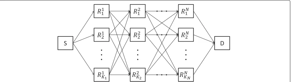
We consider a wireless network that includes a single source,Nlayers of parallel relays and a single destination. There areKnrelays available in layern. It is assumed that

every relay in our system adopts the decode-and-forward (DF) protocol and each node operates in the half-duplex mode. We denote the source as layer 0 and the destina-tion as layer(N+1). It is assumed that the nodes in the nth layer can only receive signals from the nodes in the

(n−1)th layer and transmit signals to the nodes in the

(n+1)th layer. There is no direct link from the(n−1)th layer nodes to the (n+ 1)th layer nodes, since the dis-tance between the(n−1)th layer and the(n+1)th layer is too long and there may be some obstacles between them. We denote the source asS, destination asD, and theith relay in thenth layer (n∈ {1, 2,. . .,N}) asRn_i. Besides, we assume that there areN+1 time slots for the end-to-end transmission. The system model is shown in Fig. 1.

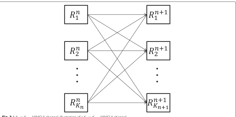
In the first time slot, the source transmits to the first layer relays using broadcasting protocol. In thenth (1 < n<N+1) time slot, the relays in the(n−1)th layer decode and forward signals to the nth layer relays. We consider aKn−1×Kn X channel in the transmission. Finally, the

(3)

Fig. 1A single-source single-destination multi-layer relay MIMO network. Illustration of a single-source single-destination multi-layer relay MIMO network

destination using multiple-accessing, and the destination could directly decode the signals. The schemes of IA and zero-forcing are used to precode and decode the signals, respectively.

We assume that there areKnrelays available in layern.

The communication channel between thenth layer relays and the(n+ 1)th layer relays is a Kn ×Kn+1 MIMO X channel where each of theKntransmitters sends a distinct

message to each of theKn+1receivers. For the cases that (i)Kn = 1 andKn+1 =1, (ii)Kn =1 andKn+1 =1, and (iii)Kn = 1 andKn+1 = 1, the communication channel between them is a broadcasting channel, multiple-access channel and point-to-point channel, respectively.

We assume each relay is equipped withMantennas. Let the number of antennas at the source and the destination to beMsandMd, respectively. We denoteHsj∈CM×Msas

the channel matrix between the source to thejth relay in the first layer. The channel matrix between theith relay in theNth layer to the destination is denoted asHid, where Hid∈CMd×M. In the middle part of the system, we denote

the channel matrix between theith relay in thenth layer to thejth relay in the(n+1)th layer asHn_ij∈CM×M. Finally, we assume that the entries ofHsj, Hn_ij, and Hid are i.i.d.

complex Gaussian random variables with zero-mean and the total power constraint of each layer isP.

3 Analysis of interference alignment

We divide the analysis of the system into three parts. In the first part, we considerKn×Kn+1MIMO X channels (for the casesKn > 1 andKn+1> 1). In the second part, we consider the broadcast channels, which are (i) from the source to the first layer relays, ifK1 >1; (ii) from thenth layer to the(n+1)th layer, ifKn = 1 andKn+1 > 1. In the third part, we consider the multiple-access channels, which are (i) from theNth layer relays to the destination, ifKN > 1; (ii) from thenth layer to the(n+1)th layer,

ifKn > 1 andKn+1 = 1. For the point-to-point MIMO channels (the caseKn = 1 andKn+1 = 1), since there is

no interference signal to be aligned, we will not consider the point-to-point MIMO channels in this section.

3.1 Kn×Kn+1MIMO X channel

3.1.1 Interference alignment scheme

Now we consider the Kn × Kn+1 MIMO X channel

between layernand layern+1 as shown in Fig. 2. We denote theith relay in layernasRn_i (i = 1, 2,. . .,Kn). If

KnorKn+1equals one, the problem reduces to a broad-casting or a multiple-accessing problem to be solved in Sections 3.2 and 3.3 In this section, we focus on the case thatKn>1 andKn+1>1.

We assume the relayRn_i is supposed to transmit mes-sagexn_ijto the relayRn_j+1, wherexn_ij ∈ CTsig×1_{is a vector}

with unit power of each component (i.e., E

xn_ijxnH_ij

= IT_sig).Tsigdenotes the degree of freedom achieved by each message.

We use V˜n_ij ∈ CM×Tsig _{to denote the transmit} beam-forming matrix, which is to map the Tsig symbols inxnij

to M antennas by the transmitter Rn_i. V˜n_ij is a full rank matrix with orthonormal columns. We rewrite the trans-mit beamforming matrix asV˜n_ij=QnVn_ij, where the matrix

Qn ∈ CM×T is also with orthonormal columns. The

matrixQnis used to (i) confine the transmit signals from each transmitter to aT-dimensional subspace; (ii) exploit the null spaces of the channel matrices to achieve higher multiplexing gain [10]. Thus, we call Qn asspace con-fining matrix. Since both V˜n_ij andQn are matrices with orthonormal columns andV˜n_ij = QnVn_ij, the columns of

Vn_ij ∈ CT×Tsig _{are also normalized and orthogonal with} each other. On the MIMO X channel, each transmitter has a distinct message for each receiver, and there are Kn+1receivers on this MIMO X channel. The signal vector transmitted by transmitterRn_i is thus:

tn_i = Kn+1

j=1 ˜

Vn_ijPn_ijxn_ij= Kn+1

j=1

(4)

Fig. 2AKn×Kn+1MIMO X channel. Illustration of aKn×Kn+1MIMO X channel

wherePn_ij ∈ CTsig×Tsig _{is the transmission power matrix.} The received signal vector for receiver Rn_j+1 can be expressed as:

Yn_j+1= Kn

i=1

Hn_ijtn_i +zn_n (1a)

= Kn

i=1

Hn_ijQnVn_ijPn_ijxn_ij+ Kn

i=1 Kn+1

m=1,m=n

(1b)

Hn_ijQnVn_imPn_imxn_im+zn_j.

The vector zn_j is a unit variance, zero mean, complex additive white Gaussian noise.

The first part of Eq. (1b) represents the desired sig-nals from allKnrelays (transmitters) in thenth layer. The

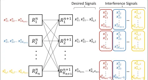
second part represents the interference signals which are supposed to be sent to the relays (receivers) other than Rn_j+1in the(n+1)th layer. For each receiverRn_j+1, there are Kndesired signals andKn(Kn+1−1)interference signals.

In this subsection, we try to find how to select trans-mit beamforming matrixV˜n_ijfor the fixed space confining matrixQn.

As shown in Fig. 3, the signals received by each receiver can be classified into two categories: desired signals and interference signals. The first part contains all the desired signals and the second part contains Kn interference

blocks, where each block includes all the interference signals coming from the same transmitter. For receiver Rn_j+1, all the interference signals should be aligned into a subspace distinct from the desired signals, such that the

interference signals can be completely canceled. There are two steps to achieve this goal.

Step I: For each receiver, we first align the interfer-ence signals coming from the same transmitter into a Tint-dimensional subspace1. In other words, according to

Fig. 3, we need to align the interference signals in the same block first.

Step II: By step I, we haveKnTint-dimensional interfer-ence subspaces for each receiver, since there areKnblocks

in a row. In this step, we let theseKnsubspaces to lie in the

sameTint-dimensional subspace. In other words, accord-ing to Fig. 3, we align the aligned blocks in a row into the same subspace. In this way, all the interference signals are aligned into the sameTint-dimensional subspace.

We know thatHn_ijQnVn_imrepresents the subspace occu-pied by the signal transmitted from the transmitterRn_i and desired by receiverRn_m+1but received by receiverRn_j+1. To realize step I, for each receiverRn_j+1, we define a series of new matricesWn_ij ∈ T×Tint _{for all}_i ∈ {_{1, 2,}. . ._,_K_n}_{, and} align all the interference signals coming from the trans-mitterRn_i (i.e.HijQnVim, ∀m∈ {1,. . .,Kn+1}, m=j) into the subspaceHn_ijQnWn_ij. The matrixWn_ijis named as inter-ference confining matrix. The selection of matrices Vn_im

should therefore satisfy the following conditions:

span(Hn_ijQnVn_im)⊂span(Hn_ijQnWn_ij),∀m ∈ {1, 2,. . .,Kn+1}, m=j.

(2)

(5)

Fig. 3Interference alignment on theKn×Kn+1MIMO X channel. Illustration of the interference alignment scheme on theKn×Kn+1MIMO X channel

After step I, for each receiver, we have aligned all the interference signals from the same transmitter into aTint -dimensional subspace. Since there areKntransmitters on

aKn×Kn+1MIMO X channel, all the interference signals for each receiver Rn_j+1 have been aligned into Kn Tint -dimensional subspaces, which areHn₁_jQnWn₁_j,Hn₂_jQnWn₂_j,

. . .,Hn_K_n_jQnWn_K_n_j. The second interference alignment step is for each receiver Rn_j+1, we let the subspaces of inter-ference signals from different transmitters lie in the same Tint-dimensional subspace2. Hence,Wnijshould satisfy the

following equation:

Hn₁_jQnWn₁_j=Hn₂_jQnWn₂_j=. . .=Hn_K_n_jQnWn_K_n_j,

∀j∈ {1, 2,. . .,Kn+1}. (3)

From Eq. (2), we know

span(Vn_im)⊂span(Wn_ij), ∀m∈ {1, 2,. . .Kn+1},m=j. (4)

Since Eq. (4) should be satisfied for all receiversRn_j+1, wherej∈ {1,. . .,Kn+1}, we can find that:

span(Vn_im)⊂span(Wn_ij), ∀j∈ {1, 2,. . .,Kn+1},j=m.

This means, for fixedVn_im, there should be some matri-cesEn_imj∈CTint×Tsig _satisfying:

Vn_im=Wn_i₁En_im₁=. . .=W_i(mn ₋₁₎En_im(m₋₁₎=Wn_i(m₊₁₎

En_im(m₊₁₎=. . .=W_iKn_n₊₁En_imK_n₊₁.

(5)

for alli∈ {1,. . .,Kn}.

We will use a 3×3 MIMO X channel as an example to illustrate how the IA scheme works in Section 3.1.2.

Since our goal is to find the matrixVn_ijwith fixed space confining matrixQnand generic channel matricesHn_ijby solving Eq. (3) and Eq. (5), we should guarantee that (i) for anyHn_ijandQn, the set of equations in (3) always have feasible solutionsWn_ijand (ii) for any series of interference confining matricesWn_ij, the set of equations in (5) always have feasible solutionsEn_imj.

By solving equations in (3) and (5), we can find thatWn_ij

is the null space ofAn_j(₋_i)(i.e.,An_j(₋_i)Wn_ij=0), where

An_j(₋_i)= ⎡ ⎢ ⎢ ⎢ ⎢ ⎢ ⎢ ⎢ ⎢ ⎢ ⎣

(I−(Hn₁_jQn)(Hn₁_jQn)†)Hn_ijQn

.. .

(I−(Hn

(i−1)jQn)(Hn(i−1)jQn)†)HnijQn (I−(Hn

(i+1)jQn)(Hn(i+1)jQn)†)HnijQn

.. .

(I−(Hn KnjQ

n_)(Hn KnjQ

n₎†_)Hn ijQn

⎤ ⎥ ⎥ ⎥ ⎥ ⎥ ⎥ ⎥ ⎥ ⎥ ⎦ ,

and En_imj (m = j) is the null space of Bn_i(₋_m_,₋_j) (i.e.,

Bn_i(₋_m_,₋_j)En_imj = 0), whereBn_i(₋_m_,₋_j)is resulted by remov-ing themth andjth sub-matrices (i.e.,(I−Wn_imWn_im†)Wn_ij

(6)

Bn_i =

Notice that in the previous notation, (·)† denotes the pseudo-inverse.

For each receiver, there are Kn desired signals andM

antennas. The number of dimensions of the whole space is therefore M. We can see the numbers of dimensions occupied by all the desired signals and interference signals areKnTsigandTint, respectively. To perfectly align all the interference signals into a subspace, which is distinct from the subspace occupied by the desired signals, the number of dimensions of the whole space should be no less than the number of dimensions occupied by all the desired sig-nals and interference sigsig-nals. Thus, we have the following condition: Bn_i(₋_m_,₋_j) correspondingly, the feasibility of equations in (3) and (5) can be always guaranteed if the size of Qn

satisfies Eq. (6) and the following conditions:

T−(Kn−1)(M−T)≥Tint, (7) Tint−(Kn+1−2)(T−Tint)≥Tsig. (8)

In following analysis and simulation, we choose the equality for Eqs. (6), (7) and (8) to maximize the degree of freedom.

Therefore, we can rewrite the received signal vector of the relayRn_j+1in Eq. (1b) as:

where the formula (9a) represents the desired signals from allKnnth layer relays. The formulas in (9b) and (9c)

repre-sents the interference signals from each transmitter. From (9b) and (9c), we can find that the interference signals from the same transmitter are aligned into the sameTint -dimensional subspace, e.g., interference signals coming from theith transmitterRn_i are aligned into the subspace

Hn_ijQnWn_ij.

We then substitute the set of equations in (3) into Eq. (9) and we can rewriteYn_j+1as:

The first part is the desired signals and the second part represents the interference signals. By now, for each receiverRn_j+1, all the interference signals are aligned into the sameTint-dimensional subspaceHn1jQnWn1j.

3.1.2 Example of the scheme: Kn=Kn+1=3

In this section, we will use a 3×3 MIMO X channel as an example to illustrate how the IA scheme introduced in Section 3.1.1 works.

In the scheme of IA, we only need to consider the subspaces occupied by the received signals, as shown in Fig. 4. For each receiver, it can receive nine signals, since Kn = Kn+1 = 3. The formulas in black are the desired signals. The formulas in the same block are the interfer-ence signals transmitted from the same transmitter, e.g., for the first receiverRn₁+1, the formulas in the red block indicate the interference signals transmitted from the first transmitterRn₁.

Recall the two steps of IA scheme introduced in Section 3.1.1. Step I: for each receiver, we need to align the interference signals in the same blocks into the subspaces pointed by corresponding arrows in Fig. 4. For example, for the first receiver Rn₁+1, we need to align the signals in the red block into the subspaceHn₁₁QnWn₁₁, align the signals in the blue block into the subspace Hn₂₁QnWn₂₁

and align the signals in the yellow block into the sub-space Hn₃₁QnWn₃₁. This step is denoted as “(i)” in Fig. 4. Step II: for each receiver, we let the interference subspaces from the first step to lie in the same subspace, e.g., for the first receiverRn₁+1, we haveHn₁₁QnWn₁₁=Hn₂₁QnWn₂₁ = Hn₃₁QnWn₃₁. This step is denoted as “(ii)” in Fig. 4.

To finish step I, from Fig. 4, we have:

(7)

Fig. 4Example of IA scheme on the 3_×3 MIMO X channel. Illustration of the two steps of IA scheme on the example of 3_×3 MIMO X channel

which means there exist a series of matricesEimjsuch that:

Vn₁₁=Wn₁₂En₁₁₂=Wn₁₃En₁₁₃, Vn₂₁=Wn₂₂En₂₁₂= Wn₂₃En₂₁₃, Vn₃₁=W₃₂n En₃₁₂=Wn₃₃En₃₁₃, (11a)

Vn₁₂=Wn₁₁En₁₂₁=Wn₁₃En₁₂₃, Vn₂₂=Wn₂₁En₂₂₁= Wn₂₃En₂₂₃, Vn₃₂=W₃₁n En₃₂₁=Wn₃₃En₃₂₃, (11b)

Vn₁₃=Wn₁₁En₁₃₁=Wn₁₂En₁₃₂, Vn₂₃=Wn₂₁En₂₃₁= Wn₂₂En₂₃₂, Vn₃₃=W₃₁n En₃₃₁=Wn₃₂En₃₃₂. (11c)

For, we need to align the interference signals from dif-ferent transmitters into the same subspace. Therefore, the selection ofWn_ijshould satisfy the following conditions:

Hn₁₁QnWn₁₁=Hn₂₁QnWn₂₁=Hn₃₁QnWn₃₁, (12a)

Hn₁₂QnWn₁₂=Hn₂₂QnWn₂₂=Hn₃₂QnWn₃₂, (12b)

Hn₁₃QnWn₁₃=Hn₂₃QnWn₂₃=Hn₃₃QnWn₃₃. (12c)

We can finally find Wn_ij by solving equations in (12). Then by solving equations in (11), we can getVn_ijfor alli andj.

3.1.3 The selection of space confining matrix:Qn

DifferentQnin the previous subsection may lead to dif-ferent results in terms of the transmission rate under a certain power constraint. Here, we propose a method to designQnin this section.

The decoding matrix used to decode the signal from the nth layer relay Rn_i to the(n+1)th layer relay Rn_j+1 is denoted byUn_ij ∈ CM×Tsig_{, which is a full rank matrix.} SinceUn_ijis the matrix used to decode signal transmitted from transmitterRn_i to receiverRn_j+1, from Eq. (10) we know that it should satisfy the conditions:

Un_ijHHn_mjQnVn_mj=0, ∀m=i, (13)

Un_ijHHn₁_jQnWn₁_j=0. (14)

With perfect IA, the transmission rate of theKn×Kn+1 MIMO X channel is represented as follows:

Kn

i=1 Kn+1

j=1

logdet(I+Un_ijHHn_ijQnVn_ijP_ijnPn_ijHVn_ijHQnHHn_ijHUn_ij).

(15)

We assume that the power is equally allocated in each layer. Then, the optimization problem corresponding to the space confining matrixQncan be formulated as fol-lows:

max

{Qn_}

Kn

i=1 Kn+1

j=1

logdet(I+Un_ijHHn_ijQnV_ijnVn_ijHQnHHn_ijHUn_ij),

s.t.

⎧ ⎪ ⎪ ⎪ ⎪ ⎪ ⎪ ⎪ ⎪ ⎪ ⎪ ⎪ ⎪ ⎪ ⎨ ⎪ ⎪ ⎪ ⎪ ⎪ ⎪ ⎪ ⎪ ⎪ ⎪ ⎪ ⎪ ⎪ ⎩

Hn_ijQnWn_ij=Hn₁_jQnWn₁_j, ∀i∈ {2,. . .,Kn};

j∈ {1,. . .,Kn+1}

span(Vn_ij)⊂span(Wn_im),∀m=j; m,j∈ {1,. . .,Kn+1};

i∈{1,. . .,Kn}

Un_ijHHn_mjQnVn_mj=0, ∀m=i; m,i∈ {1,. . .,Kn};

j∈ {1,. . .,Kn+1}

Un_ijHHn₁_jQnWn₁_j=0, ∀i∈ {1,. . .,Kn}; j∈ {1,. . .,Kn+1}.

(16)

Due to the non-convexity of the problem (16), we pro-pose sub-optimal solutions. We apply genetic algorithms [24] to find a sub-optimalQn, which provides good per-formance as shown in our simulation results.

We designed Algorithm 1 (on page 17) to solve our problem. In this algorithm, there are five steps: Initializa-tion, SelecInitializa-tion, Crossover, MutaInitializa-tion, and Termination.

(8)

sample asFn_g, whereg∈ {1, 2,. . .,G}. For each g∈ {1, 2,. . .,G}, we getQn_gas the orthonormal basis for the null space ofFn_g. Therefore, the size ofQn_gis M×T.

• Selection: we use this group ofQn_gto get the fitness value, which is the objective function in optimization problem (16):

FIT(g)= Kn

i=1 Kn+1

j=1

logdetI+U_ijnHHn_ijQn_gV_ijnVn_ijHQn_gHHn_ijHUn_ij,

(17)

and select(G−1)samples by applyingRoulette Wheel Selection and denote them as

Sn_g,g∈ {1, 2,. . .,G−1}. In this way, the one that leads to a larger fitness value is more likely to be selected. In the last step of this part, we select theFn_g that leads to the largest fitness value and denote it asSn_G. • Crossover: sinceG is an odd number, for

g∈ {1, 2,. . .,G−1}, we divideSn_g intoG−₂1pairs. In each pair, we randomly swap some parts of them. For Sn_G, we keep it unchanged.

• Mutation: for eachg∈ {1, 2,. . .,G−1}, we randomly change part ofSn_g. ForSn_G, we keep it unchanged. Let Fn_g =Sn_g, for allg∈ {1, 2,. . .,G}.

• Termination: we repeatedly run the algorithm until a fixed number of generationsσ is reached.

In Selection, we generate Sn_G with the largest fitness value and keep it unchanged in Crossover and Mutation. We do this in order to guarantee that in each generation, the largest fitness value will not decrease.

Finally, we get the space confining matrix Qn as the orthonormal basis for the null space of theFn_Gand hence can getVn_ijby solving Eqs. (3) and (5) andUn_ij by solving Eqs. (13) and (14).

Recall that our goal is to maximize the data rate of the Kn × Kn+1 MIMO X channel, which is written as Eq. (15). To maximize it,Un_ijandVn_ijshould be multiplied by the matrix whose columns are left singular vectors and the matrix whose columns are right singular vectors of

Un_ijHHn_ijQnVn_ij, respectively.

3.2 Broadcast channel

For the 1× ¯K broadcast channel, the channel gain from the transmitter to thejth receiver is denoted asHbj.Hbjis

anM×Mtmatrix, whereMandMtare the numbers of

antennas at each receiver and the transmitter, respectively.

Ubjis the decoding matrix at receiverjwith rankTsig, and Vbjis the encoding matrix used to encode the signalxbj

from the transmitter to receiverj. The received signal of receiverjis:

Yj=Hbj ¯ K

m=1

VbmPbmxbm+zbj,

Algorithm 1Genetic algorithm to find proper space con-fining matrixQn

1: INITIALIZATION

2: Initialize an odd number G and for each g ∈

{1, 2,. . .,G}randomly generate an(M−T)×Mmatrix

Fn_g. Set GENERATION=0.

3: repeat

4: SELECTION

5: forg=1;g≤G;g+ +do 6: Qn_g =null(Fn

g).

7: For alli ∈ {1, 2,. . .,Kn}andj∈ {1, 2,. . .,Kn+1}, getWn_ijfrom Eq. (3), getVn_ijfrom Eq. (5) and get

Un_ijfrom Eq. (13) and Eq. (14).

8: Get Fitness Value FIT(g).

9: end for

10: Get the Select Function:

RATE(0)=0,

RATE(g)= g

m=1FIT(m) _G

m=1FIT(m)

, ∀g∈ {1, 2,. . .,G}.

11: forg1=1;g1≤(G−1);g1+ + do

12: Randomly generate a real numbert∈[ 0, 1). 13: forg2=1;g2≤G;g2+ + do

14: ifRATE(g2−1)≤t<RATE(g2)then

15: LetSn_g₁ =Fn_g₂.

16: end if

17: end for

18: end for

19: Find theFn_g that gives the largest FIT(g). LetSn_G = Fn_g.

20: CROSSOVER

21: We randomly divide Sn₁,S₂n,. . .,Sn_G₋₁ into

G−1

2 pairs. For each pair, we randomly

gen-erate (M − T) numbers tj ∈ {1, 2,. . .,M}

(j=1,. . .,M−T) and swap the entities at positions {(1,t1),(2,t2),. . .,(M−T,tM−T)}of them.

22: MUTATION

23: forg=1;g≤G−1;g+ +do

24: Randomly generate (M − T) numbers tj ∈

{1, 2,. . .,M} (j = 1,. . .,M − T). Replace the entities at positions{(1,t1),(2,t2),. . .,(M− T,tM−T)}ofSngwith(M−T)randomly generated

Gaussian complex numbers with zero-mean.

25: end for

26: For allg∈ {1, 2,. . .,G}, letFn_g =Sn_g.

27: GENERATION=GENERATION+1.

28: untilGENERATION=σ.

wherePbmis the power allocation matrix.

Since there are M antennas at each receiver,zbj is an

(9)

= ˜

coordinate transformation under the basisV˜bj. For each

receiver, to maximize the received signal UH_bjHbjVbjPbj,

which is equivalent toUH_bjHbjV˜bjTbjPbj, the decoderUbj

and the coordinate transformation matrixTbjshould be

the left and right singular matrix ofHbjV˜bj.

Then we can achieve the optimal solution by rewrit-ing the iterative algorithm given in [25] as shown in Algorithm 2.

The convergence of the algorithm has been proved in [25].

The data rate received by thejth receiver of the broad-casting part is

log(det(I+UH_bjHbjVbjPbjPHbjVHbjHHbjUbj))=

log(det(I+bjPbjPHbjHbj)),

(18)

wherebjis a diagonal matrix:

bjUH_bjHbjV˜bjTbj.

3.3 Multiple-access channel

Similar to the broadcast channel, for theK¯ ×1 multiple-access channel, the channel gain from theith transmitter to the receiver is denoted as Him. Him is an Mr × M

matrix, where Mr and M are the numbers of antennas

at the receiver and each transmitter respectively. Theith transmitter transmitsxim with the precoding matrixVim

and the power allocation matrixPimto the receiver. Then, the destination decodes the received signalYm by using the decoding matrixUim, where

Ym= ¯ K

i=1

HimVimPimxim.

Same as the broadcast channel, the following condition should be satisfied to perfectly align the interference:

span(Uim)=nullSH_im,

whereSimis defined as follows:

Sim

H1mV1m,. . .,H(i−1)mV(i−1)m,H(i+1)mV(i+1)m, . . .,H_{K m}¯ V_{K m}¯ .

⎢

⎣ b(j+1) :

UH bK¯(n)HbK¯

⎥ ⎦

and obtainV˜bjas the orthonormal basis for the

null space ofSbj. Calculate SVD ofHbjV˜bjto get

the updatedUbj(n+1)andTbj.

5: end for

6: n=n+1.

7: untilK_j¯₌₁Ubj(n+1)−Ubj(n) ≤.

LetU˜im be the orthonormal basis for the null space of SH_im. We have an equation as follows:

Uim= ˜UimRim,

whereRim denotes the span matrix ofUim˜ . We can find the optimal solution ofUimandVimby using the previous algorithm. The transmission rate of theith transmitter of this channel is

logdetI+UH_imHimVimPimPHimVHimHHimUim

= log(det(I+imPimPHimHim)),

(19)

where the diagonal matriximis

im=RH_imU˜H_imHimVim.

4 Power allocation

In this section, we first find space confining matrixQnby using Algorithm 1 in Section 3.1.3 under the condition of equal power allocation and then try to optimize the power allocation without changingQn.

(10)

there areKnrelays in thenth layer andKn+1relays in the

According to the number of relays in each layer, there are four kinds of channels in the whole system: point-to-point MIMO channel, broadcast MIMO chan-nel, multiple-access MIMO chanchan-nel, and Kn × Kn+1 MIMO X channel. In the following, we discuss them one by one.

4.1 Point-to-point MIMO channel

In this subsection, we consider a point-to-point MIMO channel with channel matrix H. The optimal decoding matrixUand encoding matrixVshould be the singular value decomposition (SVD) ofH. Then, the transmission rate of this channel is

log(det(I+UHHVPPHVHHHU)),

where

tr(PPH)≤P.

Water-filling algorithm can be used to achieve the opti-mal power allocation.

4.2 Broadcast and multiple-access MIMO channel

Since the optimization of power allocation in multiple-access channel is similar to that in the broadcast channel, in this section, we only talk about the optimization of the 1× ¯Kbroadcast MIMO channel.

For broadcast MIMO channel, we use the method shown in Section 3.2 to select precoding matrices and decoding matrices. The data rate received by the jth receiver is

log(det(I+UH_bjHbjVbjPbjPHbjVHbjHHbjUbj)), (22)

where Pbj is the power allocation matrix for signals desired by receiverj.

With the assumption of equal receiving rate of each receiver in the same layer and the objective to maxi-mize the transmission rate of this broadcast channel, the

optimization problem can be formulated as follows

maximize

entity ofPbjaspbji. The objective function of Eq. (23) can

be rewritten as

Total power used in this channel is

¯

The optimization problem can be rewritten as follows

maximize

which is a geometric programming problem. The geo-metric programming problem can be transferred into a convex problem [26], and the optimal solution can be obtained by numerical method, e.g., the Matlab software CVX [27].

4.3 Kn×Kn+1MIMO X channel

(11)

m=1

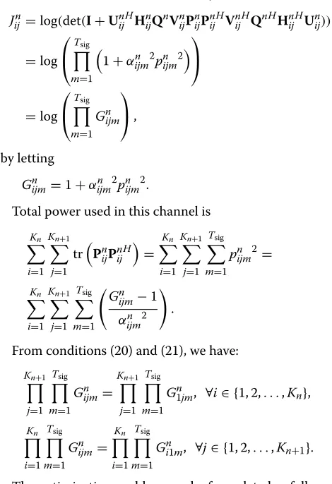
by letting

Gn_ijm=1+α_ijmn 2pn_ijm2.

Total power used in this channel is

Kn

From conditions (20) and (21), we have:

Kn+1

The optimization problem can be formulated as follows

maximize

which is also a geometric programming problem.

5 Performance evaluation

We divide this section into three parts. Firstly, we evaluate the performance of Algorithm 1, which is a genetic algo-rithm used to find proper space confining matrixQnin the IA scheme of MIMO X channel. Secondly, we show the

gains, i.e., modeling the entries ofHn_ijas independent and identical (i.i.d.) complex Gaussian random variables with zero mean.

5.1 Performance of Algorithm 1

For theKn×Kn+1MIMO X channel, we use Algorithm 1 to select the space confining matrixQn. We evaluate the performance of Algorithm 1 with difference number of generationsσ and different sizes of groupsG.

Several MIMO X channels with different channel sizes are studied. With fixed size of groupG=11, Fig. 5 shows the transmission rates versus number of generations σ. Figure 6 shows the transmission rates versus group size Gwith fixed number of generationsσ = 15. The trans-mission powerPused in both figures are 40 dB. From the figures, we can see that (i) the transmission rate is increas-ing with both the number of generations and the group size and (ii) when the number of generations reaches 15 or the group size reaches 11, there is no significant change in the transmission rate. Therefore, in Sections 5.1 and 5.3, we set the number of generationsσas 15 and set the group sizeGas 11.

Number of Generations σ

Transmission Rate in bits per use

2x3 MIMO X channel 3x4 MIMO X channel 4x5 MIMO X channel 5x6 MIMO X channel

(12)

0 20 40 60 80 100 20

30 40 50 60 70 80 90 100 110

Group Size G

2x3 MIMO X channel 3x4 MIMO X channel 4x5 MIMO X channel 5x6 MIMO X channel

Fig. 6Evaluation of Algorithm 1 with different sizes of groupsG. Results for evaluation of Algorithm 1 with different sizes of groupsG

5.2 Comparison between MIMO X channel and MIMO

interference channel

In this subsection, we will first compare the performance

of the IA scheme for the Kn × Kn+1 MIMO X

chan-nel with that of the IA scheme presented in [28] for the Kn × Kn+1 MIMO interference channels in our corre-sponding conference paper [20]. Secondly, we analyze the computational complexity of these two IA schemes in the corresponding wireless channels.

5.2.1 Performance of MIMO X channel and MIMO interference channel

The interference channel is a kind of channel with mul-tiple transmitter-receiver pairs, where each transmitter only wants to send message to its corresponding receiver. For the benchmark of theKn×Kn+1MIMO interference channel, we assume each transmitter selects one distinct relay as its receiver. We compare the transmission rate of theKn×Kn+1MIMO interference channel with ourKn×

Kn+1 MIMO X channel. Since each transmitter selects one distinct receiver on the MIMO interference channel, in our simulation, we show two ways for the transmitters to choose receivers: (i) for each transmitter, it randomly select a distinct receiver and (ii) throughout all the pos-sible selection combinations, we select the one that gives the largest transmission rate of the channel. We call the case “(i)” as interference channel without selection and the case “(ii)” as interference channel with selection.

The overall transmission rate of the system is limited by the bottleneck, which is the layer with the minimum transmission rate. The system we investigate is a multiple-layer-multiple-relay system, in reality, it is rarely possible that the numbers of available relays in all layers are equal. Comparing with our MIMO X channel, the shortcoming of the MIMO interference channel is the transmission rate

of adjacent layers with different numbers of transmission relays and receiving relays. Since each transmitter should select one distinct receiver for the MIMO interference channel, there will be an under-utilization of relays in the layer with more relays.

In Figs. 7 and 8, two MIMO channels with different sizes, 2×3 and 3×4, are studied. From both the figures, we can see that the transmission rate of the MIMO X channel is around 40 % higher than the interference chan-nel with relay selection and around 55 % higher than the interference channel without relay selection.

5.2.2 Complexity analysis

On MIMO X channel, the computation of the IA scheme mainly lies in the selection of space confining matrixQn. In the part of selection of Qn, we introduced a genetic algorithm (i.e., Algorithm 1). For each Qn in Algorithm 1, we need to find its fitness value as defined in Eq. (17). The complexity of finding the fitness value is dominated by finding the matricesWn_ijand matricesEn_im₁4, which are the null space ofAn_j(₋_i)andBn_i(₋_m_,₋₁₎, respectively.

To find the complexity of getting An_j(₋_i), we firstly need to find the complexity of calculating the matrix

I− (H1jQn)(H1jQn)†

HijQn, which is a sub-matrix in

the matrix An_j(₋_i). For an m × n matrix A, an n × p matrixBand anm×mmatrixC, the complexity of cal-culating the multiplication of A and B is O(mnp) [29] and the complexity of calculating the inverse of matrix

C is O(m3) [30]. Thus, the complexity of getting I− (H1jQn)(H1jQn)†

HijQnisO(5M2T+M3). SinceT ≤M, we can writeO(5M2_T ₊_M3₎_as_O₍_M3₎_{. The complexity} of calculating the matrixAn_j(₋_i)is thereforeO(M3_K_n)_{. By} the same analysis, the complexity of calculating the matrix

Bn_i(₋_m_,₋₁₎isO(M3Kn+1). Hence, the complexity of getting

0 5 10 15 20 25 30 35 40 45

0 5 10 15 20 25 30

Transmission Power in dB

MIMO X channel

MIMO interference channel with selection MIMO interference channel withoutselection

(13)

0 5 10 15 20 25 30 35 40 45 0

10

Fig. 8Comparison between 3×4 MIMO X channel and 3×4 interference channel. Results for comparison between 3×4 MIMO X channel and 3×4 interference channel

matricesW_ijnfor alli ∈ {1,. . .Kn}andj∈ {1,. . .Kn+1}is O(M3Kn2Kn+1)and the complexity of getting the matri-ces Eim1 for all i ∈ {1,. . .Kn} and m ∈ {1,. . .Kn+1} isO(M3KnKn+12). The complexity of finding the fitness value is thenO(max{Kn,Kn+1}M3KnKn+1). The number of calculations of the fitness value is determined by the number of generations multiplied by the size of group in Algorithm 1. By setting size of the group to 11, from the simulation results in Figs. 5 and 6, we can find that the number of generations is a relatively small value, i.e., less than 20.

For theKn×Kn+1MIMO interference channel, a dis-tributed algorithm is introduced to realize the interference alignment. However, the complexity of the distributed algorithm is unknown, since as the channel size increases, the rate of convergence is still an open problem [28].

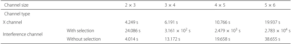
Nevertheless, we can compare the complexity of MIMO X channel and MIMO interference channel through numerical results (i.e., running time). Table 1 demon-strates the comparison of the running time for the two wireless channels.

From the table, we can find that the running time of the MIMO X channel is almost in the same order of mag-nitude with the running time of the MIMO interference

5.3 Evaluation of the whole system

We evaluate the performance of our system in data rate with two benchmark systems: (i) multiple layers of par-allel relays system with only one relay in each layer and (ii) the system built by replacing the MIMO X channels in our proposed system with MIMO interference channls and uses the IA algorithm presented in [28] to design transceivers.

In Figs. 9 and 10, we plot the transmission rates versus the transmission power of one layer. There are three lay-ers of relays, and the numblay-ers of relays in the laylay-ers are 3−2−3. The comparison between our system and sys-tem “(i)”, where only one relay can be used in each layer, is shown in Fig. 9. We can see that the transmission rate of our system, which uses all available relays in each layer, is around 40 % higher than that of system “(i)”. The insight is, by using multiple relays in each layer, we can increase the DoF of the middle part of system, and hence increase the transmission rate of the whole system.

In Fig. 10, we compare our system with system “(ii),” which is built by replacing the MIMO X channels in our proposed system with MIMO interference channels. We have shown the MIMO interference channel of system “(ii)” in our corresponding conference paper [20], where each first layer relay should select a distinct second layer relay. In that system, there are two cases: interference channel without selection and interference channel with selection.

From Fig. 10, we can see that due to the inequality of the relays in each layer, the transmission rate of our system with MIMO X channels is 52 and 66 % higher than the sys-tem with MIMO interference channels with and without selection, respectively.

Table 1Comparison in running time between the MIMO X channel and interference channel

Channel size 2×3 3×4 4×5 5×6

Channel type

X channel 4.249 s 6.191 s 10.766 s 19.937 s

Interference channel With selection 24.086 s 3.161×10

2_s _2.479_×₁₀3_s _2.783_×₁₀4_s

(14)

0 5 10 15 20 25 30 35 40 45 0

5 10 15 20 25 30

Use all available relays in each layer Select 1 relay per layer

Fig. 9Comparison between our system and the system selecting one relay in each layer. Results for comparison between our system and the system selecting one relay in each layer

6 Conclusions

In this paper, we studied the relay network consisting of multiple layers of relays with multiple antennas. We divided the system into three parts, consisting of broad-cast channels, multiple-access channels, and MIMO X channels. For the broadcast and multiple-access chan-nels, we optimized the precoder and decoder of each transmitter and receiver under the condition of interfer-ence alignment. For the MIMO X channels, we designed transmit and receive beamforming matrices based on IA technique. Furthermore, we generalized the power con-straint from node level to layer level in system evaluation and determined the power allocation of all nodes. Finally, we evaluated the performance of our system and two

0 5 10 15 20 25 30 35 40 45

0 5 10 15 20 25 30

MIMO X channel

MIMO interference channel with selection MIMO interference channel withoutselection

Fig. 10Comparison between our system and the system with MIMO interference channel. Results for comparison between our system and the system with MIMO interference channel

benchmark systems and showed that our system could achieve around 40 % higher transmission rate.

Endnotes

1_{In the following of this paper, we call it as a} _T int -dimensionalinterference subspace.

2_Hn

ijQnWnijis the subspace of interference signals from

transmitterRn_i received by receiverRn_j+1 3_{The conditions} ₍_K

n−1)(M−T) < T and(Kn+1− 2)(T −Tint) < Tintshould be satisfied to guarantee the existences ofWn_ijandEn_jmn, sinceWn_ijandEn_imj are in the null space ofAn_j(₋_i)andBn_i(₋_m_,₋_j), respectively.

4_{According to Eq. (5), we can find that}_Vn

im=Wni1Enim1. In order to getVn_im, we only need to calculateEn_im₁rather thanEimjfor allj∈ {1, 2,. . .Kn+1}.

Received: 29 February 2016 Accepted: 5 September 2016

References

1. A Ibrahim, A Sadek, W Su, K Liu, Cooperative communications with relay-selection: when to cooperate and whom to cooperate with? IEEE Trans.Wireless Commun.7(7), 2814–2827 (2008)

2. X Liang, S Jin, X Gao, K-K Wong, Outage performance for

decode-and-forward two-way relay network with multiple interferers and noisy relay. IEEE Trans. Commun.61(2), 521–531 (2013)

3. Y Sagar, J Yang, H Kwon, inProc. of IEEE Vehicular Technology Conference (VTC). Capacity of a modulo-sum arbitrary SISO relay network (IEEE, Yokohama, 2012), pp. 1–5

4. W Tam, T Lok, T Wong, Flow optimization in parallel relay networks with cooperative relaying. IEEE Trans. Wireless Commun.8(1), 278–287 (2009) 5. A Behbahani, R Merched, A Eltawil, Optimizations of a MIMO relay

network. IEEE Trans. Signal Process.56(10), 5062–5073 (2008) 6. S Borade, L Zheng, R Gallager, Amplify-and-forward in wireless relay

networks: rate, diversity, and network size. IEEE Trans. Inf. Theory.53(10), 3302–3318 (2007)

7. O Popescu, C Rose, D Popescu, inProc. of IEEE GLOBECOM. Signal space partitioning versus simultaneous water filling for mutually interfering systems, vol. 5 (IEEE, Dallas, 2004), pp. 3128–3132

8. R Menon, A MacKenzie, J Hicks, R Buehrer, J Reed, A game-theoretic framework for interference avoidance. IEEE Trans. Commun.57(4), 1087–1098 (2009)

9. V Cadambe, S Jafar, Interference alignment and degrees of freedom of the K-user interference channel. IEEE Trans. Inf. Theory.54(8), 3425–3441 (2008)

10. M Maddah-Ali, A Motahari, A Khandani, Communication over MIMO X channels: interference alignment, decomposition, and performance analysis. IEEE Trans. Inf. Theory.54(8), 3457–3470 (2008)

11. S Jung, J Lee, inProc. of International Symposium on Personal Indoor and Mobile Radio Communications (PIMRC)). Interference alignment and cancellation for the two-user X channels with a relay (IEEE, London, 2013), pp. 202–206

12. C Suh, D Tse, inProc. of 46th Ann. Allerton Conf. Commun., Control and Computing. Interference alignment for cellular networks (IEEE, Monticello, 2008), pp. 1037–1044

13. V Ntranos, M Maddah-Ali, G Caire, Cellular interference alignment. IEEE Trans. Inf. Theory.61(3), 1194–1217 (2015)

14. N Chiurtu, B Rimoldi, I Telatar, inProc. of IEEE Int. Symp. Inf. Theory (ISIT). On the capacity of multi-antenna Gaussian channels, vol. 53 (IEEE, Washington, 2001)

(15)

of wireless X networks. IEEE Trans. Inf. Theory.55(9), 3893–3908 (2009) 22. C Huang, V Cadambe, S Jafar, Interference alignment and the generalized

degrees of freedom of the X channel. IEEE Transa. Inf. Theory.58(8), 5130–5150 (2012)

23. A Agustin, J Vidal, inProc. of IEEE Inf. Theory Workshop (ITW). Degrees of freedom of the rank-deficient MIMO X channel (IEEE, Seville, 2013), pp. 1–5 24. L Davis,Handbook of genetic algorithms. (Van Nostrand Reinhold, New

York, 1991)

25. Z Pan, K-K Wong, T-S Ng, inIEEE Trans. Wireless Commun. Generalized multiuser orthogonal space-division multiplexing, vol. 3, (2004), pp. 1969–1973

26. S Boy, L Vandenberghe,Convex optimization. (Cambridge University Press, Cambridge, 2004)

27. M Grant, S Boyd, CVX: Matlab software for disciplined convex programming [Online]. Available: http://stanford.edu/~boyd/cvx Dec. 2008

28. K Gomadam, V Cadambe, S Jafar, A distributed numerical approach to interference alignment and applications to wireless interference networks. IEEE Trans. Inf. Theory.57(6), 3309–3322 (2011)

29. C Sun, Y Yang, Y Yuan, Low complexity interference alignment algorithms for desired signal power maximization problem of MIMO channels. EURASIP J. Adv. Signal Process.2012(1), 1–13 (2012)

30. GH Golub, CF Van Loan,Matrix computations, vol. 3. (JHU Press, Baltimore, 2012)

Submit your manuscript to a

journal and beneﬁ t from:

7Convenient online submission 7Rigorous peer review

7Immediate publication on acceptance 7Open access: articles freely available online 7High visibility within the ﬁ eld

7Retaining the copyright to your article