Experimental evaluation of interference alignment for broadband WLAN systems

R E S E A R C H

Open Access

Experimental evaluation of interference

alignment for broadband WLAN systems

Christian Lameiro

, Óscar González

, José A. García-Naya

, Ignacio Santamaría

and Luis Castedo

Abstract

In this paper, we present an experimental study on the performance of spatial interference alignment (IA) in indoor wireless local area network scenarios that use orthogonal frequency division multiplexing (OFDM) according to the physical-layer specifications of the IEEE 802.11a standard. Experiments have been carried out using a wireless network testbed capable of implementing a 3-user MIMO interference channel. We have implemented IA decoding schemes that can be designed according to distinct criteria (e.g., zero-forcing or MaxSINR). The measurement methodology has been validated considering practical issues like the number of OFDM training symbols used for channel estimation or feedback time. In case of asynchronous users, a time-domain IA decoding filter is also compared to its frequency-domain counterpart. We also evaluated the performance of IA from bit error ratio measurement-based results in comparison to different time-division multiple access transmission schemes. The comparison includes single- and multiple-antenna systems transmitting over the dominant mode of the MIMO channel. Our results indicate that spatial IA is suitable for practical indoor scenarios in which wireless channels often exhibit relatively large coherence times.

Keywords: Interference alignment; WLAN systems; OFDM; Interference channel; Testbed

1 Introduction

Interference management is a key issue in the design of wireless systems. When several users transmit over the same wireless resources, orthogonal access tech-niques such as frequency-division or time-division mul-tiple access (FDMA and TDMA, respectively) are tra-ditionally applied to avoid interference among them. In orthogonal multiple access schemes, the system band-width and/or time resources are divided among users and the individual data rates decrease with the network size. Interference alignment (IA) has been recently proposed as an alternative interference management method that con-fines interference signals within half of the signal space at each receiver, hence allowing each user to transmit over the interference-free subspace [1].

Although a large number of theoretical results have shown IA to be a very promising technique, there is still lack of experimental over-the-air (OTA) results evaluat-ing its actual performance in real wireless scenarios. This scarcity of experimental results is mainly due to the high

*Correspondence: [email protected]

1Department of Communications Engineering, University of Cantabria, Santander, Spain

Full list of author information is available at the end of the article

costs and effort required to conduct OTA measurements in IA scenarios. For example, to evaluate the practical performance of spatial IA methods, at least six nodes (three transmitters and three receivers) with two antennas each are needed to implement the simplest multiple-input multiple-output (MIMO) interference channel.

1.1 Previous experimental work on IA

The first work that tackled a real-world implementation of IA was presented in [2]. This work considered the implementation of IA techniques combined with cancel-lation methods over a wireless network testbed comprised of 20 Universal Software Radio Peripheral (USRP) nodes equipped with two antennas each. The implemented tech-nique does not correspond to pure IA because it requires a certain amount of cooperation among access points in such a way that all the network interferences can be nulled out. Several practical issues were addressed in this work, showing that IA is unaffected by frequency off-sets or by the use of different modulations. Imperfect time synchronization, however, affects IA but this issue can be overcome by performing IA at the sample level, i.e., before demodulation and synchronization takes place. Finally, this work posed the interesting question of how to

perform sample level alignment in orthogonal frequency division multiplexing (OFDM) systems over frequency-selective channels.

IA was further evaluated in [3], where the authors con-ducted an experimental study over measured indoor and outdoor MIMO-OFDM channels. By modifying the dis-tance among network nodes and antennas, they character-ized the effect of spatial correlation and subspace distance and showed that IA is able to achieve the maximum available degrees of freedom (DoF) over realistic chan-nels. However, although the channels were obtained from measurements, no OTA transmissions of aligned signals were actually measured. Therefore, many practical issues such as time/frequency synchronization, imperfect chan-nel state information (CSI), and dirty radio-frequency (RF) effects such as phase noise, non-linearities, IQ imbal-ance, or clipping and quantization in the digital-to-analog and analog-to-digital converter (DAC/ADC) were not taken into account. In [4], different IA schemes are eval-uated in the 3-user single-input single-output (SISO) interference channel using frequency extensions. As in [3], the results in [4] were obtained using urban macro-cell measured channels but without transmitting aligned signals.

In [5–7], the first aligned real transmissions were con-ducted to evaluate spatial-domain IA in a 3-user interfer-ence channel, thus providing more precise results about the actual performance of IA in realistic scenarios. In [5], the feasibility of spatial IA over indoor channels and single-carrier transmissions was studied, identifying also some practical issues that affect IA performance already pointed out in [2] and [3]. In addition, the CSI estima-tion error was also described as an important issue that was further analyzed in [6]. The 3-user MIMO interfer-ence channel with OFDM transmissions is also studied in [7], along with coordinated multi-point transmission methods. In this work, RF impairments are identified as an important source of mismatch between practical and theoretical performance of IA. However, the work in [7] focuses on verifying simulation models and no analysis of the inherent limitations of IA is performed.

The work in [8] described two real-time implementa-tions of IA in a 3-user MIMO-OFDM scenario showing that the computational power of current embedded plat-forms makes software-defined implementations of IA fea-sible. Another approach was followed by the authors of [9], where blind IA was implemented with the aim of avoiding the intense global CSI requirements of spatial-domain IA.

Recent experimental evaluations of spatial interference alignment analyze the main performance limiting fac-tors found in real-world scenarios [10], study the impact of outdated channel state information [11], consider its combination with antenna selection techniques [12],

or consider analog feedback in a distributed real-time implementation [13].

1.2 Summary of key practical issues arising when implementing IA techniques

Despite the promising theoretical results on IA, several practical impairments come up in real scenarios that might degrade the overall system performance. In the fol-lowing, we detail the main issues affecting practical IA transmissions.

1.2.1 Imperfect CSI

IA is usually studied assuming perfect CSI is available at every node of the network, a premise that never occurs in practice. Moreover, since the computation of the pre-coders and depre-coders involves all the pairwise interference channels, even a slight time variation of a single channel would ideally result in a change of all IA precoders and decoders. In practice, this causes two problems. First, the presence of channel estimation errors or time variations makes it impossible to perfectly suppress interference [5, 6]. Second, nodes must exchange its local CSI to com-pute the IA solution, and this introduces additional over-head and delay between channel estimation and data transmission. During this elapsed time, the channel may vary, hence out-dating the CSI estimates especially when there are moving scatterers in the surroundings. Besides CSI estimation errors, dirty RF effects [14] are also res-ponsible for a great portion of the gap between ideal and practical setups. Major contributors to distortion in OFDM systems are nonlinear amplifiers, clipping, ADC effects, and phase noise. Some of these effects have been modeled in [7].

1.2.2 Signal collinearity

Even under the unrealistic assumption that perfect CSI is available, the received signal is projected into the sub-space orthogonal to the interference in order to null the interferences once they are aligned. In this process, part of the desired signal energy is lost due to spatial collinearity between signal and interference subspaces. In the pres-ence of high spatial collinearity, the desired signal power is severely reduced. To overcome this problem, many algo-rithms have been proposed to reach a trade-off between signal and interference power, such as the MaxSINR algo-rithm [15] considered in this work. Recent works have also suggested the use of antenna switching strategies [12, 16, 17].

1.2.3 Synchronization

802.11a waveform — with a bandwidth of 20 MHz — for the three users. Assuming that the same wave-form (including training and/or preamble sequences) is employed at the three transmitters, we then distinguish two different cases with respect to synchronization:

I) All users are perfectly synchronized in time and frequency. This means that the three transmitters transmit exactly at the same time instants, while the three receivers are able to perfectly acquire the time and frequency references of its corresponding transmitter before processing the received signals. Another possibility would consist in assigning orthogonal training sequences to all users. Given that the transmitters operate synchronously, each receiver acquires the time reference with respect to its desired transmitter without being affected by interferences. II) All users operate asynchronously in an

uncoordinated way, leading to symbol timing offsets between the desired and the interfering OFDM symbols. Consequently, each receiver has to acquire the time and frequency reference from the received signal, which consists of the desired signal plus the interference from two of the three transmitters. Therefore, the signal-to-interference noise ratio (SINR) at the input of the receiver decreases with respect to case I. Notice that assigning orthogonal training sequences to the users does not alleviate the problem because now the transmission of those orthogonal sequences is not synchronous. Consequently, it cannot be guaranteed that the observed training sequence at the receiver is not affected by interferences from the other users.

With respect to spatial interference alignment, pre-coding at the transmitter and depre-coding at the receiver can be performed in the frequency domain (the usual approach in the literature) or in the time domain, lead-ing to a set of four different possibilities to apply spatial interference alignment precoding and decoding. Notice that, as shown in [18], interference leakage at the OFDM receiver is completely independent of the delays between the transmitters and the receivers only if spatial interfer-ence alignment precoding and decoding operations are carried out in the time domain. Otherwise, the magnitude of the interference leakage will depend on to the delays between transmitters and receivers. Even if those delays are apparently small (e.g., 2 samples at 40 MHz sampling frequency yielding 50 ns due to an imperfect synchro-nization among the three transmitters), they may produce interference leakage after decoding at the receiver. The imperfect cancelation occurs when some samples of the undesired users adjacent OFDM symbols interfere the current one due to an insufficient cyclic prefix (CP) length

or time misalignments. This is because the frequency-domain IA scheme is designed to cancel the interference when the system can be equivalently decomposed into a set of non-overlapping channels. If this is not the case, there will be inter-symbol and inter-carrier interference (ISI and ICI, respectively) components in the interfering signals that cannot be eliminated.

Spatial interference alignment decoding in the time domain consists in filtering the received signal in the time domain. On the other hand, time-domain decoding can-not effectively suppress all the interference because of the resulting filter length. The length of this filter can easily introduce inter-symbol interference as it may exceed the CP length minus the channel delay spread [18].

Therefore, interference can be completely suppressed at the receiver only when interference alignment precoders and decoders are applied at the frequency domain on a per-subcarrier basis, hence demanding for a synchronous scenario.

Contrarily, if a fully synchronous scenario is not fea-sible, the SINR at the input of the receiver decreases due to the high level of interference. On the other hand, it is well known that the performance of syn-chronization tasks depends on the SINR at the receiver input, and therefore their performance will improve if the SINR is increased by reducing the level of inter-ference. This can be achieved by applying interference alignment decoding in the time domain at the receiver input, before the synchronization tasks. However, there is a trade-off between the level of symbol inter-ference introduced by the time-domain filtering and the multiuser interference-suppression capacity. The longer the interference-suppression filter in the time domain, the higher the inter-symbol interference and the lower the interference leakage.

1.3 Contributions

In this paper, we extend our work in [5, 6] to broad-band OFDM wireless transmissions. Specifically, we use the IEEE 802.11a wireless local area network (WLAN) physical-layer standard [19] as a benchmark to evaluate the performance of spatial IA in an illustrative indoor sce-nario. The measurement setup can be thought of as an indoor WLAN system in which three access points — with two antennas each — communicate simultaneously over the same frequency (channel resource) with three static devices (e.g. laptops), also equipped with two anten-nas each. This is opposed to conventional WLAN systems that would assign different channels to each communi-cation link (i.e., FDMA). The goal of this paper is to evaluate experimentally several spatial IA schemes in indoor WLAN applications, identifying and analyzing the main issues that degrade their performance in broadband OFDM transmissions, and comparing their end-to-end measurements with those of TDMA-based schemes. In this work, we only consider systems in which each user transmits a single stream of data to its intended receiver. More specifically, the main contributions of this work are the following:

• With respect to our previous work in [5] and [6], in which only single-carrier transmissions over flat-fading channels were considered, here the experimental work focuses on OFDM transmissions based on the 802.11a standard and with a 20-MHz bandwidth. Broadband transmissions pose new difficulties but also permit the implementation of more complex IA schemes. Additionally, we have improved our measurement methodology and we have also reduced the time elapsed between channel estimation and IA transmission from 5 s in [5] and [6] to a second.

• As discussed previously, we consider and compare the performance of spatial IA decoding schemes that operate either in time domain [18, 20] or in a more conventional per-subcarrier basis in frequency domain. Furthermore, we have assessed the actual performance of IA and MaxSINR schemes [15]. • Additionally, we analyze the main issues that might

affect our measurement methodology (see Section 5) and consequently our results, such as the number of training symbols used for channel estimation or the feedback time elapsed between training and transmissions of aligned frames.

• Finally, we present error vector magnitude (EVM) and bit error ratio (BER) measurement-based results for different data rates. We also compare them to those obtained when TDMA-based transmissions are employed. The comparison includes SISO and MIMO systems transmitting over the dominant

mode of the MIMO channel (referred to as dominant eigenmode transmission or DET [21]).

Taking into account all pros and cons outlined in Section 1.2.3, we always apply the spatial interference alignment precoders at the transmitters in the frequency domain on a per-subcarrier basis, while the three trans-mitters and receivers are synchronized between them in time (up to 2 samples at 40-MHz sampling frequency) and in frequency due to the following reasons:

1. to keep the feedback time short (and with low variability) during the measurements;

2. to employ the same transmit waveform for the three users (i.e., training signals do not depend on the number of users);

3. to reuse (without a significant performance degradation) conventional time and frequency synchronization algorithms valid for OFDM-based wireless systems in single-user interference-free scenarios;

4. to be able to compare the performance of spatial interference alignment decoding at the receiver applied in time with respect to when it is applied in frequency under the following conditions:

(a) the same set of spatial interference alignment precoder and decoder vectors (i.e., the same interference alignment solution) is employed; (b) the aforementioned interference alignment

solution was computed from the same channel realization;

(c) the same set of acquired frames experiencing the same channel realizations is used to estimate the considered figures of merit (EVM, BER) when interference alignment decoding is applied in time domain or in frequency domain;

(d) time synchronization is performed when interference alignment is applied in time domain and reused for the frequency-domain case, hence the performance of the frequency-domain interference alignment decoding is not degraded because of the interference.

for the application of the spatial interference alignment problem (high SNR at the receiver and interference lev-els compared to those of the desired signals, see Fig. 11). Finally, the validity of the above-mentioned measurement methodology is also analyzed to ensure that our compari-son is not affected by insufficient training (see Fig. 14) or by excessive feedback time (see Fig. 15).

The rest of the paper is organized as follows. Section 2 describes spatial IA in a 3-user 2×2 MIMO-OFDM chan-nel considering both post-FFT and pre-FFT IA decod-ing schemes. In Section 3, the wireless network testbed utilized for the measurements is briefly described. Mea-surement setup and methodology are both explained in Sections 4 and 5, respectively. The obtained results are discussed in Section 6. Finally, Section 7 concludes the paper.

2 Spatial interference alignment

IA is able to exploit the multiple time, frequency, and spa-tial dimensions available in a wireless system. However, when aligning over the frequency or time domain, the number of required dimensions to arbitrarily approach to the maximum DoF promised by IA grows exponentially with the number of users [22]. The number of required dimensions, on the contrary, is considerably less when aligning interference over the spatial dimension [23, 24]; which facilitates its practical implementation. For instance, for a 3-user channel, 3n+1 symbols can be trans-mitted using 2n+ 1 extensions, where n is an integer, yielding a total of(3n+1)/(2n+1)DoF [1]. This would require a theoretically infinite number of frequency domain extensions to achieve the maximum number of 3/2 DoF in the 3-user SISO interference channel, while spatial domain IA is able to achieve the maximum number of 3 DoF with constant channels and two anten-nas. Furthermore, IA by means of symbol extensions requires significant multipath [25, 26], whereas a suffi-cient antenna separation ensures no DoF loss when IA is performed in the spatial domain. Another advantage of spatial IA is that it can be readily applied while being compliant with any OFDM signaling format such as the 802.11a WLAN standard, as shown in this paper. On the contrary, any alignment scheme over time or frequency would require major changes on the physical layer format. Further, we focus on the 2×2 MIMO 3-user interference channel because it can be easily implemented with the multiuser MIMO testbed described in Section 3.

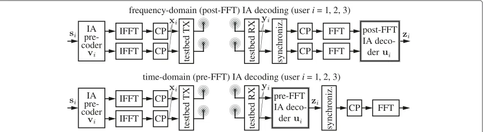
This section reviews the concept of IA in the spatial domain and discusses the application and design of IA decoders in the time and in the frequency domain. How-ever, as commented in Section 1.3, in all experimental evaluations, the IA precoders were always applied at the transmitters before the IFFT on a per-subcarrier basis in the frequency domain, whereas at the receivers, the

decoders are applied either in the time domain (pre-FFT decoding) or in the frequency domain (post-(pre-FFT decoding).

2.1 Interference alignment with post-FFT decoding

Let us consider a 3-user MIMO interference channel comprised of three transmitter-receiver pairs (links) that interfere with each other as shown in Fig. 1. Each user is equipped with two antennas at both sides of the link and sends a single stream of data. Following the convention introduced in [27], this interference network is denoted as (2×2, 1)3. Assuming a fully coordinated scenario in which all users transmit their OFDM symbols exactly at the same time instants or when the possible delays among users can be accommodated by the CP minus the channel delay spread, each receiver can use a conventional synchronizer and, consequently, the IA decoder can be applied after the FFT block on a carrier-by-carrier basis (see top of Fig. 2).

Assuming that the CP is sufficiently long to accommo-date the channel delay spread, the discrete-time signalyi at theith receiver for a given subcarrier (to not overload the notation unnecessarily, the index denoting the subcar-rier is omitted in this section) is the superposition of the signals transmitted by the three users, weighted by their respective channel matrices and affected by noise, i.e.,

yi =Hiixi+

j=i

Hijxj+ni, (1)

wherexi ∈C2×1is the signal transmitted by theith user,

Hijis the 2×2 flat-fading MIMO channel from transmit-terjto receiveri, andni ∈ C2×1is the additive noise at receiveri.

2.1.1 Closed-form interference alignment solution

Spatial IA uses a set of beamforming vectors (pre-coders){vi ∈C2×1}and interference-suppression vectors (decoders) {ui ∈ C2×1} that must satisfy the following zero-forcing conditions for all transmitter-receiver pairs

i=1, 2, 3:

uH_i Hiivi =0

uH_i Hijvj=0,∀j=i. (2)

There is an analytical procedure to obtain precoders and decoders for the(2×2, 1)3case [1]:

1. The precoder for user 1,v1, is any eigenvector of the following2×2matrixE(each eigenvector yields a different IA solution):

E=(H31)−1H32(H12)−1H13(H23)−1H21. (3) 2. The precoders for users 2 and 3,v2andv3, are

respectively obtained as

Fig. 1Scheme of the₍2_×2, 1₎3_{interference network. Direct channel links are shown inblack solid lineswhereas interference channels are plotted in} gray dashed lines

v3=(H23)−1H21v1. (5) SinceEis a full-rank2×2matrix with probability one for generic MIMO channels, in which each entry of the channel matrix is an independent and

identically distributed random variable drawn from a continuous distribution, it has two eigenvectors that can be chosen as the precoder for the first user, hence yielding two distinct IA solutions. An interesting fact of the 3-user interference channel is that it induces a permutation structure and, consequently, the procedure described above leads to exactly the same set of IA solutions regardless of the user employed for starting the procedure. In summary, there are only two different IA solutions per subcarrier. 3. Finally, the interference-suppression filters

(decoders) are designed to lie in the orthogonal subspace of the received interference signal, i.e., the decoder of user 1 is the eigenvector of

[H12v2, H13v3]associated with the zero eigenvalue. The decoders for users 2 and 3 are obtained in an analogous way.

When zero-forcing IA linear precoders and decoders are applied at both sides of the link, the signal received by theith user is given by

zi = uHi Hiivisi+

j=i

uH_i Hijvjsj+uHi ni

= uH_i Hiivisi+uHi ni, (6)

wheresiis the transmitted symbol corresponding to the

ith user. Notice that the signal from theith transmitter to theith receiver travels over the equivalent SISO chan-neluH_i Hiivi. The interference terms are totally suppressed when projecting the received signal onto the subspace whose basis isui.

Similarly to forcing channel equalization, zero-forcing IA suffers from noise amplification when MIMO channels are close to singular. Other approaches can be used to mitigate this limitation and perform better in the medium and low signal-to-noise ratio (SNR) regimes. One such example is the MaxSINR algorithm [15] which has

also been adopted in the measurements of this work for comparison purposes.

2.1.2 MaxSINR algorithm

The MaxSINR algorithm aims at maximizing the SINR at each receiver by a proper design of the precoding and decoding vectors. As a result, it usually outperforms pure IA for medium and low SNR values, whereas it approaches IA as the SNR increases. To compute such precoders and decoders, an alternating optimization algorithm must be applied. Thereby, the decoders (precoders) are optimized at each iteration while the precoders (decoders) are kept fixed. This results in a closed-form solution at each step of the algorithm. The MaxSINR algorithm can then be summarized as follows.

1. While the precoders are kept fixed, choose the decoder of each user as the one that maximizes the SINR: eigenvector of the matrix pencil(A,B)with

maximum generalized eigenvalue, andIis an identity matrix with the appropriate dimensions.

2. Keeping the decoders fixed and changing the roles of transmitters and receivers, the precoders are obtained as those maximizing the SINR of the reversed communication, i.e.,

3. Steps 1 and 2 are repeated until convergence or until a prescribed number of iterations has been reached.

For further details, we refer the reader to [15].

2.2 Interference alignment with pre-FFT decoding

As mentioned in Section 1.2.3, the existence of symbol timing offsets between the desired and the interfering OFDM symbols impairs the synchronization procedure. Therefore, interference must be eliminated (or at least suf-ficiently reduced) in asynchronous scenarios before the synchronization step. To this end, pre-FFT IA decoders must be applied at the receiver side. Let us first con-sider a general time-domain spatial interference align-ment approach in which both precoders and decoders are applied in time domain,vj[n]∈C2×1, n=0,. . .,L−1, is the impulse response of the linear precoder with lengthL

for the transmitterj, andui[n]∈ C2×1, n=0,. . .,L−1, is the impulse response of the pre-FFT linear decoder for receiveri, also with lengthL. The output signal at receiver

i,zi, is given by

where n is the discrete-time sample index, xj[n] is the discrete-time OFDM signal transmitted by userj,Hij[n] is the matrix impulse response of the frequency-selective MIMO channel between transmitterjand receiveri,μij denotes the delay between transmitter j and receiver i, and∗denotes convolution. The received signal at useriis also affected by an additive, spatially, and temporally white Gaussian noiseni[n]∼N(0,σ2I). Notice that we are now considering an asynchronous wireless system and, for this reason, a delay μij is explicitly introduced in the signal model given by Eq. (9).

As we already showed in [18], the interference leakage when precoding and decoding that are both applied in the time domain is given by the sum of the energies of the equivalent interference channels,uH_i [−n]∗Hij[n]∗vj[n] with i = j. In other words, the interference leakage is independent of the specific delays between users,μij, and hence this approach can work properly in the presence of symbol timing offsets. Note that for the interference to be mitigated before time synchronization, only time-domain decoders are strictly necessary, while precoders could be applied either in the time or in the frequency domain. Clearly, by precoding in the frequency domain, the interference leakage will depend on the delays between transmitters and receivers, and hence there will be some residual interference when the interfering symbols are not aligned in time with the receiver window. Nevertheless, this simple scheme makes time synchronization possi-ble in the presence of asynchronous interferences and allows us to assess the performance degradation of time-domain decoding with respect to its frequency-time-domain counterpart.

in [18, 20], would outperform the adopted approach but at the cost of an increased computation time for calculating the set of interference alignment precoders and decoders, thus impacting the feedback time. In any case, the design and evaluation of such approaches is beyond the scope of this paper.

A schematic of the pre-FFT IA decoding scheme is shown in Fig. 2 (bottom). Assuming again perfect CSI knowledge, we propose the following method for comput-ing the pre-FFT IA decoders:

• First, the IA precoders and decoders are computed on a per-subcarrier basis applying the closed-form solution described in Section 2.1.1.

• Next, aNFFT-point IFFT is applied to the set of

post-FFT decoders in order to obtain their impulse response.

• Finally, the pre-FFT filters are truncated to a given length,L, so as to reduce the ISI and ICI.

Note that the shorter the impulse response of the equiv-alent channel — consisting of the actual wireless channel convolved with the pre-FFT filters — the lower the ISI/ICI but the higher the residual multiuser interference (MUI) and vice versa. Thus, pre-FFT filtering involves a trade-off between both sources of interference [18].

It is important to notice that the OFDM (2 × 2, 1)3

interference channel is being interpreted as NFFT

paral-lel single-carrier(2×2, 1)3interference channels and that there exist two IA solutions per subcarrier. Thus, there is a total of 2NFFT _{solutions in the OFDM case,}1_{as each}

of theNFFTsubcarriers can use a different solution

with-out altering the alignment conditions. However, as we are interested in pre-FFT filters with an impulse response as short as possible (and, consequently, pre-FFT filters with a frequency response as smooth as possible in the frequency domain), it is important to select those solutions that pro-vide the smoothest frequency response for the equivalent channel. Simulations have shown that there are only two sets of smooth solutions out of 2NFFT_{. Figure 3 plots the}

magnitude of the frequency responses of one of the SISO equivalent channels obtained after calculating the IA pre-coders and depre-coders using one of these sets (empty circles) and the other one (full circles), respectively. Note that any other combination of these two sets leads to more abrupt changes in the frequency response.

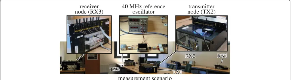
3 Multiuser MIMO testbed

This section describes the MIMO wireless network testbed that has been used to assess, in a realistic sce-nario, the IA techniques presented in the previous section. Both transmit and receive testbed nodes (see Fig. 4) have a quad dual-band front-end from Lyrtech, Inc. [28]. This RF front-end can use up to eight antennas that are connected to four direct-conversion transceivers by

means of an antenna switch. Each transceiver is based on Maxim [29] MAX2829 chip, which supports both up and down conversion operations from either 2.4–2.5 GHz or 4.9–5.875 GHz. The front-end also incorporates a pro-grammable variable attenuator to control the transmit power value. The attenuation ranges from 0 to 31 dB in 1 dB steps, while the maximum transmit power declared by Lyrtech is 25 dBm per transceiver.

The baseband hardware is also from Lyrtech. More specifically, each node is equipped with a VHS-DAC mod-ule and a VHS-ADC modmod-ule, respectively, containing eight DACs and eight ADCs. Each pair of DAC/ADC is connected to a single transceiver of the RF front-end and the signals are passed in I/Q format.

Both transmit and receive nodes employ buffers that are dedicated to store the signals to be sent to the DACs as well as the signals acquired by the ADCs. The utilization of such buffers allows for the transmission and acquisi-tion of signals in real-time, while the signal generaacquisi-tion and processing is carried out offline. Both baseband hardware and RF front-ends of the transmit nodes are synchronized in time and in frequency by means of two mechanisms:

• Transmit nodes implement a hardware trigger attached to the real-time buffers and to the DACs and ADCs. When one of the nodes fires the trigger (usually the node corresponding to user 1) for all buffers, DACs and ADCs receive the signal and start transmission and acquisition simultaneously (the timing between nodes is precise up to 2 samples, hence resulting in an error upper bound of±50 ns). • The sampling frequency of DACs and ADCs is set to

40 MHz, while the RF front-ends support a reference frequency of 40 MHz. In order to synchronize all nodes in frequency, the same common external 40 MHz reference oscillator is distributed to the DACs, ADCs and RF front-ends of all nodes, hence guaranteeing high-quality frequency synchronization.

Fig. 3Example of the set of equivalent channels obtained with each solution in the frequency domain from simulated wireless channels. Notice that there are only two smooth sets out of 2NFFT

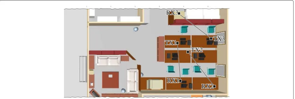
4 Measurement setup

Figure 5 shows the measurement scenario setup at the University of Cantabria to recreate a typical 3-user indoor interference channel. The access to the room was care-fully controlled during the measurements to ensure that there were no moving objects in the surroundings. Addi-tionally, we also checked that no other wireless system was operating in the 5-GHz frequency band. All nodes were equipped with monopole antennas at both transmit-ter and receiver sides [31, 32], while the antenna spacing was set to approximately 7 cm (forced by the separation of the antenna ports at the RF front-end).

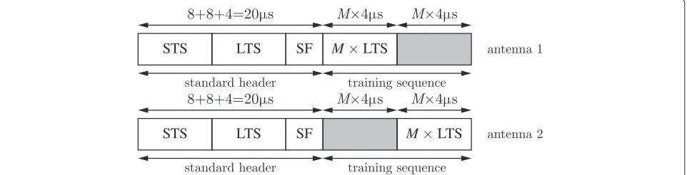
We followed the IEEE 802.11a WLAN standard with the conventional frame structure and synchronization head-ers. Figure 6 shows the 802.11a physical-layer frame. The header comprises the short training sequence (STS), the

long training sequence (LTS), and the signal field (SF). The STS is used for frame detection, while the LTS is utilized for frequency offset correction and channel equal-ization. The SF contains information about the data rate and the frame length. During our experiments, the frame length remained constant and there was no rate adap-tation. Therefore, we made no use of the information conveyed by the SF.

Each OFDM symbol contains 48 data symbols and 4 pilots, which were OFDM-modulated using a 64-point IFFT. The CP length is 16 samples (800 ns).

Figure 7 shows the general block diagram of a transmit-ter chain which differs from that of a conventional 802.11a in the IA precoding block and in the utilization of two transmit antennas. Both software and hardware elements perform the following steps:

Fig. 5Plan of the measured scenario. The distances between users 1, 2, and 3 are approximately 3, 3.4, and 3.2 m, respectively. Notice that the line-of-sight of the link between TX3 and RX3 is blocked by shelves

• The source bits are encoded (convolutional code, scrambling, and interleaving) and mapped to a BPSK, QPSK, 16-QAM, or 64-QAM constellation (see “FEC” and “symbol mapper” blocks in Fig. 7) depending on the transmission rate according to the 802.11a standard (cf. [19]). The data frame length is set to a reasonable length for a WLAN frame (1250 bytes), which depending on the transmission rate translates into a different number (denoted byN in Table 1) of OFDM data symbols.

• An IA precoder is applied to each subcarrier and two OFDM symbols (one for each antenna) are generated. • At each antenna, the OFDM-sampled symbols are

encapsulated into 802.11a standard-compliant frames and afterwards they are upsampled by a factor of two. • The resulting signals are scaled so as to have a mean

transmit power of 5 dBm per antenna, quantized according to the 12-bit resolution of the DACs, and finally stored in the real-time buffers available at the transmit nodes of the testbed.

• At this point, the transmitters are ready to receive the trigger signal and start transmitting simultaneously. Once the transmit nodes are triggered, the buffers containing the OFDM signal are read by the

corresponding DACs at a rate of 40 Msample/s. Next,

the analog signals are sent to the RF front-end in order to be transmitted at the center frequency of 5610 MHz. Simultaneously, the three receivers start to acquire the transmitted frames.

Figure 8 shows the hardware and software elements cor-responding to a receiver implementing pre-FFT decod-ing. Notice the position of the IA decoder block, which is applied in time domain before synchronization takes place, as explained in Section 2.2. The pre-FFT IA decoder generates one stream of data that is subsequently pro-cessed following a typical 802.11a receiver structure. The block diagram corresponding to post-FFT decoding is analogous to the transmitter shown in Fig. 7 and does not require an additional description.

The trigger signal is received by both transmitters and receivers simultaneously. When triggered, the receive nodes carry out the following operations:

• The RF front-end down-converts the signals received by the selected antennas to the baseband, generating the corresponding I and Q analog signals.

• All I and Q signals (four in total) are then digitized by the ADCs at a sample rate of 40 Msample/s and they are stored in the real-time buffers.

Fig. 7Block diagram of hardware and software elements at each transmit node. IA precoding is performed before the IFFT

• The I and Q signals are decimated by a factor of two. • The signals are properly scaled according to the 12

bits ADC resolution. Notice that this factor is constant during the course of the whole

measurement, thus not affecting the properties of the wireless channel.

• (Only for pre-FFT decoding) The acquired signals are processed by the pre-FFT IA decoder which

generates a single data stream to be processed by a standard 802.11a receiver.

• Frame detection and time synchronization take place. • The frame is properly disassembled, and the OFDM

symbols are parallelized and synchronized in frequency.

• The 64-point FFT is applied. Only once for pre-FFT decoded frames and twice for post-FFT decoded frames. Note that if the IA decoder is applied at the frequency domain (post-FFT), then the signals coming from the two receive antennas are processed

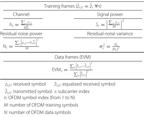
Table 1Formulas applied to training or data frames for obtaining the different parameters

Residual noise power Residual noise variance

Ns=

zs,n: received symbol ¯zs,n: equalized received symbol ◦

zs,n: transmitted symbol s: subcarrier index n: OFDM symbol index (from 1 to N)

M: number of OFDM training symbols

N: number of OFDM data symbols

separately, including the FFT operation, up to the point in which the IA decoding is applied. • (Only for post-FFT decoding) frequency-domain

symbols are processed by the post-FFT IA decoder which generates a single data stream for the next processing blocks.

• The next step is least squares channel estimation and zero-forcing equalization.

• Finally, a symbol-by-symbol hard decision decoding is performed followed by a channel decoder which outputs the estimated transmitted bits.

5 Measurement methodology

Success in the experimental evaluation of wireless com-munication systems relies mainly on the utilized measure-ment methodology, which depends on the scenario and the methods to be assessed. Given the complexity of the setup (see Fig. 1) the correct design of the measurement methodology is even more critical. In order to perform a fair comparison, it is necessary that the measurement methodology supports the assessment of several figures of merit, with and without interference, while guaranteeing that in both cases the signals experience the same chan-nel realization. The methodology should also allow us to measure the amount of interference created by each user as well as the interference leakage.

Fig. 8Block diagram of hardware and software elements at each receive node. IA decoding is performed before the FFT

to that exhibited by other alternative approaches, all of them experiencing the same channel realization (notice that the wireless channel can be estimated free of inter-ference and in an independent way for each transmission scheme in order to verify that all schemes experienced the same channel realization).

To conduct the training stage, we have introduced the training frame shown in Fig. 9, whose format differs from that of the IEEE 802.11a standard. In the following, we detail the measurement procedures performed at each stage.

• Training stage: all users sequentially send over each transmit antenna training frames comprised ofM long-training OFDM symbols in a TDMA fashion (only a single user is transmitting at a given time instant), while the three receivers are simultaneously acquiring. Once the training signals have been acquired, the nine pairwise MIMO channels are estimated and the precoders and decoders for each transmission scheme are computed.

• Data transmission stage: users transmit data frames comprised ofN OFDM symbols according to different transmission schemes. Signals

corresponding to the following schemes are sent one after each other (without delays between them):

1. IA transmission: all users transmit simultaneously, hence creating a 3-user interference channel. The IA precoders are applied at the transmitter in the frequency domain right before the FFT.

2. Perfect IA transmission: each user applies the same set of precoders as in the previous scheme, next the resulting signals are transmitted in a sequential fashion, i.e., from only one user at a time. This transmission scheme enables us to measure the residual interference level created by each transmitter at each receiver. In other words, we are able to evaluate the impact of the residual interference by comparing the actual performance during the IA stage with that in the absence of interference.

3. MaxSINR transmission: all users transmit simultaneously, creating again a 3-user interference channel. The IA precoders and decoders are computed with the MaxSINR algorithm, as explained in Section 2.1.2. The noise variance has been obtained according to Table 1, and the algorithm has proceeded until

convergence with a random initial point. While IA focuses exclusively on canceling the interference without paying attention at the quality of the resulting equivalent channel, MaxSINR trades

interference mitigation and desired signal enhancement, which may provide a performance improvement if the SNR is not sufficiently high for IA to be optimum.

4. DET-TDMA transmission: users transmit sequentially through the principal eigenvectors of the channel. This scheme is sometimes denoted as dominant eigenmode transmission (DET) [21] and provides the best equivalent channel response. Therefore, it allows us to evaluate the degradation of the desired links when all available antennas are entirely employed for interference mitigation. 5. SISO-TDMA transmission: users transmit

sequentially using a single antenna for transmission and reception, hence creating a standard-compliant 802.11a link. In the experiments, each transmitter uses the first antenna while both antennas are sequentially used for reception. This strategy provides data

transmitted over two different SISO channel realizations and more accurate results after averaging.

For each channel realization, the foregoing procedure is repeated for all individual data rates specified by the IEEE 802.11a standard. Therefore, a training stage followed by a data transmission stage is conducted for each data rate. Notice that the medium access control (MAC) layer in the IEEE 802.11a standard adapts the data rate according to the quality of the received signal. In our experiments, however, we fix the rate regardless of the reception quality.

6 Results

6.1 Characterization of the channel realizations

In order to ensure statistically representative results, we conducted a sufficiently large number of executions of the aforementioned procedure over different wireless chan-nels. In particular, binary switches allowed us to choose four different two-antenna sets at each node which makes a total of 4096 different channel realizations (all chan-nels are available for download in the web page of the COMONSENS project [30]). The estimated RMS delay spread for all channel realizations is 180.7 ns, which is a relatively long delay spread but in accordance with val-ues reported by the TGn channel models [33]. Note that the corresponding interference alignment solution is com-pletely different as long as a single channel coefficient of the three channel matrices changes. We recall that the position of the nodes nor the transmission frequency were changed.

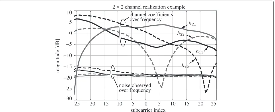
First of all, we characterized the quality of the channels in our setup. In Fig. 10, we provide an example of the fre-quency response magnitude (normalized by the average of the channel amplitudes) for one of the measured 2×2

MIMO channels. Figure 10 also plots the estimated noise power at each receive antenna obtained as indicated in Table 1. Notice that we can obtain four noise variance esti-mates, one for each transmit-receive antenna pair. It can be observed that the noise level is not flat over frequency and follows the quality of the corresponding channel coef-ficient, i.e., it is proportional to the channel gain. This behavior is explained by signal distortion at the transmit-ter, also referred to as transmitter noise [34]. Hereinaftransmit-ter, we will refer to this estimated noise as residual noise according to the way it is calculated.

Then, we define the signal-to-residual noise ratio (SRNR) as the ratio between the estimated signal power and the residual noise power. Notice that the SRNR serves as a pessimistic proxy for the SNR as it accounts for the combined effect of the thermal noise at the receiver and the signal distortion at the transmitter. Figure 11 shows the estimated probability density function (PDF) of the SRNR at each receiver for both the desired and the interfering links. The SRNR for each subcarrier has been obtained with the expressions indicated in Table 1. As shown in the figure, the SRNRs range from approx-imately 15 to 30 dB, with significant differences among receivers: interference is slightly stronger than signal at receivers 1 and 3, whereas receiver 2 experiences higher signal strength.

These measurements demonstrate the suitability of the scenario for the evaluation of IA techniques: first, all desired and interfering signals are of comparable strength and, second, SRNRs are relatively high.

6.2 Comparison of pre-FFT and post-FFT IA decoding

In this section, we experimentally evaluate the perfor-mance of the pre-FFT (time-domain) IA decoding scheme proposed in Section 2.2 in comparison to post-FFT (frequency-domain) decoding while at the transmitter, IA precoding is applied in the frequency domain and the three transmitters are synchronized among them. All OTA transmissions are carried out at 24 Mbit/s (16-QAM) and the EVM of the received signal constellation (calculated as in Table 1) is used as the performance metric.

Fig. 10Example of one of the 2×2 MIMO channels obtained in the measurement scenario. The four noise estimates that were obtained using the four SISO links are also depicted in the figure. Notice that the noise power is not flat over frequency and varies according to the amplitude of the corresponding channel coefficient

summed up to yield a received signal comprised of the three time-misaligned frames. In order to ensure that the desired signals are entirely affected by interference, we apply such a time delay as a cyclical shift, increasing the total length of the received signal accordingly. Note that the resulting SRNR will be approximately 4.7 dB lower, since the noise is also added up in this process. Never-theless, the relative performance of pre-FFT and post-FFT IA decoding will not be noticeably affected by such SRNR reduction. We plot in Fig. 12 the estimated median EVM of the received constellation for M = 30 training sym-bols and a decoder length ofL = 30 samples. It can be observed that the EVM of the post-FFT decoding scheme degrades as the delay increases, which is the result of the aforementioned synchronization issues inherent to the post-FFT approach. On the contrary, the pre-FFT decod-ing scheme exhibits an EVM almost independent from the time delay. Finally, the third curve labeled as “sync-aided

IA post-FFT decoding” shows the EVM of the post-FFT decoding scheme when the time synchronization is per-fect (no time synchronization tasks are performed, since the optimum delay is known beforehand it is directly applied at the receiver), and the resulting EVM is similar to that of the pre-FFT scheme.

To further evaluate the pre-FFT IA decoding scheme, we will focus on the synchronized setting in the remainder of this section. We first study the impact of the pre-FFT decoder length on the performance of IA which, as men-tioned in Section 2.2, involves a trade-off between ISI and residual MUI. To this end, we evaluate the EVM of the received signal constellation when MUI is suppressed with both post- and pre-FFT decoders. Training frames consist

ofM=30 training OFDM symbols per transmit antenna.

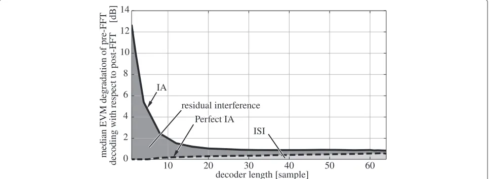
Figure 13 shows the median EVM degradation of the pre-FFT technique for different decoder lengths, L ∈[1, 64], with respect to the post-FFT decoder which obviously

Fig. 12Median EVM with respect to the transmit delay between transmit users for both pre- and post-FFT decoding as well as the so-called “sync-aided IA post-FFT decoding” corresponding to perfect time synchronization at the receiver with post-FFT decoding (M=30,L=30, 16-QAM). The delay between the transmitters has been emulated using the perfectly synchronized received signals during the perfect IA transmission stage

provides the best performance. In order to demonstrate the ISI versus residual MUI trade-off, the comparison has been carried out for both IA and perfect IA transmis-sions. For perfect IA, the degradation is only due to ISI and, as expected, it increases with the decoder length. On the other hand, a shortened IA decoder cannot prop-erly suppress the MUI leading to a high degradation of the constellation EVM. As the decoder length increases, however, the amount of MUI is greatly reduced whereas the degradation due to ISI grows at the rate seen in the perfect IA curve. This analysis illustrates the existing ISI-MUI trade-off from which it turns out that a good choice for the decoder length would be 30 taps. This decoder length will be used in the remaining experiments since it provides slightly less than 1 dB of EVM degradation

(whereof around 0.3 dB are due to ISI) with the advan-tage of a reduced receiver complexity and the possibility to perform frame synchronization in totally unsynchronized scenarios (as revealed in Fig. 12).

Secondly, we evaluate the effect that the quality of the CSI has on the performance of aligned transmissions con-sidering our setup. In Fig. 14, we show the evolution of the EVM for different numbers of OFDM training sym-bols. From the two upper curves (corresponding to IA transmissions), it can be observed that a small number of training symbols, below 20 or 30, does not provide an accurate CSI and leads to a significant degradation of the EVM due to interference. On the other hand, a number of training symbols above 30 does not improve the EVM anymore, which leads to a constant degradation between

Fig. 14Evaluation of the median constellation EVM with the number of OFDM training symbols used in the training stage (L=30, 16-QAM)

perfect IA and IA of around 4 dB. The fact that the EVM does not improve when increasing the number of train-ing symbols suggests that the performance of IA is not only limited by imperfect CSI but also by other spuri-ous effects, such as those derived from reusing the same training sequence and thus exciting the same nonlineari-ties each time. Notice also that the gap between post-FFT and pre-FFT decoding is substantially higher for IA than for perfect IA. This is due to the fact that, for the latter case, the degradation between both decoding schemes is caused by the additional ISI introduced by the pre-FFT decoding process (since the MUI has been avoided by sequential transmissions), whereas for the former case is due to ISI and residual MUI (see Fig. 13). Additionally, the impact of transmitter noise is also lower for perfect IA since a single user is transmitting at a time instead of three simultaneously, as in the case of pre-FFT or post-FFT IA. One possible source of degradation could be the chan-nel variations between the training stage and the data transmission stage, since the channel estimates used to compute the IA precoders and decoders are outdated by the time the aligned precoded transmission is actually performed. To evaluate this hypothesis, we conducted an additional experiment where a deliberate feedback time was introduced.2The results in Fig. 15 show that increas-ing feedback time does not cause additional degradation of the received signal EVM, hence proving the channel remains static for at least 10 s. Notice, however, that the performance could improve for feedback times shorter than a second, which we cannot measure. This is con-sistent with the special care taken to guarantee that our measurement scenario is completely static (see Section 4). From the results shown in Fig. 15, we can ensure the valid-ity of our measurement methodology regardless of the feedback time.

Once both the hypotheses of having inaccurate and out-dated CSI estimates have been ruled out, there are still other reasonable effects which may jointly limit the per-formance of IA and may not completely disappear when using a large number of pilot symbols.

The impact of non-linearities in power amplifiers and RF oscillator phase noise on IA was empirically evaluated in [7]. When the signal distortion occurs at the trans-mitter, it is known as a transmitter noise and leads to spatially colored noise at the receiver. Transmitter noise, also referred to as dirty RF, is specially important when the transmitter and the receiver are close to each other since its effect is directly proportional to the channel power gain. Section 6.1 shows that transmitter noise is present in our measurement campaign. Its detrimental impact on the performance of MIMO systems is already well-known and has been empirically studied in [34–36]. Some other effects, such as amplification gain drift (also known as transmitter droop) [37] and packet-to-packet power vari-ations, have not been studied yet in the context of IA. Notice that these effects may be specially pernicious for spatial-domain IA since they lead to power fluctuations at the transmitter over time which are different for every antenna and packet and therefore cannot be fought with training.

Fig. 15Evaluation of the median constellation EVM with the feedback time (M=30,L=30, 16-QAM). The feedback times are intentionally introduced and are ranging from 1 to 10 s, approximately

delay between the incoming desired and interfering sig-nals. However, a careful experimental analysis of this issue and how largely it affects IA is still necessary and we leave it as a future work.

Finally, in view of the results in Figs. 13 and 14, we have chosen the parameters which provide a nearly optimal performance with a reasonable complexity, that is,M =

30 training symbols and a decoder length ofL=30 sam-ples. The cumulative distribution function (CDF) of the received constellation EVM obtained with this parameter setup is shown in Fig. 16. It is shown that the perfor-mance loss caused by moving from a frequency-domain

to a time-domain decoder is always below 1 dB for IA and below 0.5 dB for perfect IA (while, in both cases, IA precoders are applied in the frequency domain at the transmitter). As a counterpart, time-domain IA decoding has the advantage that no inter-user time synchronization is required. Additionally, these differences are negligible compared to the roughly 4-dB difference between perfect IA and IA schemes shown in Fig. 16.

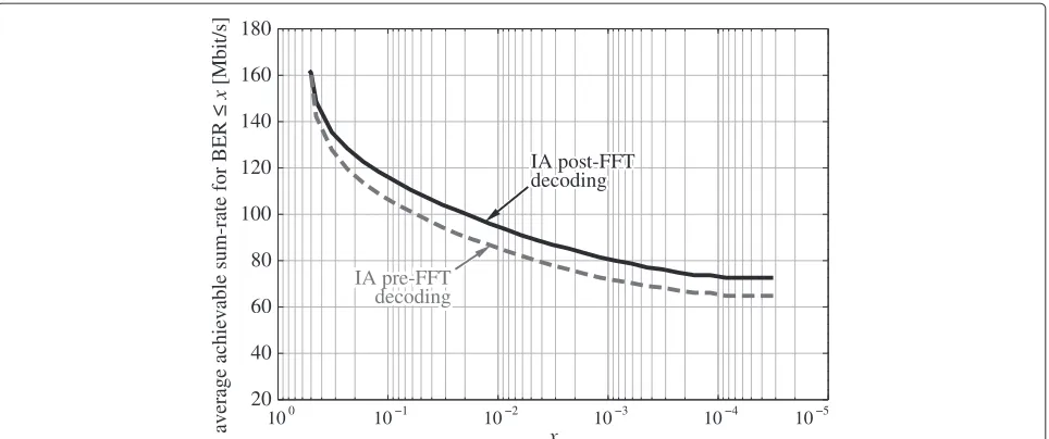
Alternatively, we show BER results for both approaches in Fig. 17. This figure represents the average achievable sum-rate that guarantees a BER equal to or lower than a given value. For each channel realization, the achievable

Fig. 17Average achievable sum-rate that guarantees a given BER for pre-FFT and post-FFT decoding methods (M₌30,L₌30)

sum-rate is obtained assuming an optimal MAC layer which selects for each user the maximum rate that satis-fies the required BER. It is important to notice that results in Fig. 17 do not take additional overhead or higher-level issues into account and they only suggest how the optimum performance of such schemes would be. The dif-ference of 1 dB in terms of EVM between time-domain (pre-FFT) and frequency-domain (post-FFT) IA decoding (shown in Figs. 13, 14, and 15) translates into a noticeably higher gap in terms of sum-rate, as shown in Fig. 17. Note also that more sophisticated algorithms may help reduce the gap between pre-FFT and post-FFT, but this analysis is out of the scope of the paper and we leave it as future work.

6.3 Comparison of the adopted schemes

In this subsection, we compare the performance of the five adopted schemes using two different metrics. With respect to IA, in this subsection, we only consider post-FFT (frequency-domain) IA decoding. First, we show in Fig. 18 the CDF of the received signal constellation EVM. As expected, DET-TDMA provides the lowest EVM and

guarantees an EVM better than −15 dB for all channel

realizations, whereas IA ensures the same signal quality in 60 % of the realizations. On the other hand, Fig. 18 also shows a noticeable degradation of IA with respect to per-fect IA, where the latter is able to achieve the same EVM value of−15 dB in a 20 % more of channel realizations. This effect was already observed in Fig. 16 and is due not only to channel estimation errors, which avoid the inter-ference to be perfectly nulled out, but also to transmitter noise and synchronization issues, as already explained in Sections 6.1 and 6.2. Alternatively, the MaxSINR scheme provides little EVM improvement over IA, increasing

the percentage in only 4 % at −15 dB. This suggests

that the operating SNRs are sufficiently high for IA to achieve good performance, and therefore MaxSINR algo-rithm converges to the zero-forcing IA solution in most subcarriers. However, when there exists high collinear-ity between the signal and the interference subspaces, MaxSINR enhances the desired channel, thus providing an improvement in the average EVM performance. Finally, it is worth mentioning that the quality of the equivalent channels after applying the IA precoders and decoders, which is represented by the EVM performance of perfect IA, is more spread than that of SISO channels. This is a reasonable result since IA precoders and decoders are independent of the desired links, hence yielding collinear-ity as well as orthogonalcollinear-ity between the signal and the interference subspaces with the same probability.

Finally, Fig. 19 shows the BER results for the five adopted schemes. We observe that IA schemes achieve higher throughput than TDMA schemes for all BER require-ments. For instance, IA provides an average rate of

73 Mbit/s with a maximum BER of 10−4, whereas SISO

Fig. 18Estimated CDF of the received signal constellation EVM for all the adopted transmission schemes (M=30,L=30)

IA, which evidences once again the significant impact of practical impairments such as channel estimation errors, transmitter noise, and imperfect timing. Such impair-ments, along with collinearity issues, significantly limit the performance of IA schemes (specially as the num-ber of users increases) and should be considered in future theoretical IA designs.

7 Conclusions

In this paper, we have presented an experimental per-formance evaluation of spatial IA in the 3-user MIMO-OFDM interference channel and considering an static indoor wireless local area network scenario. We have carefully analyzed the main practical impairments that

may degrade the end-to-end performance: imperfect CSI, frame detection in asynchronous scenarios, and dirty RF effects. To this end, we have deployed a suitable experi-mental setup made up of three MIMO transmitters and receivers and measured received constellation EVM and BER for a set of indoor channels following the conven-tional frame structure and synchronization strategies of the IEEE 802.11a WLAN standard. We have firstly pointed out that time-domain IA decoding must be applied in totally asynchronous scenarios to cancel out the interfer-ence before time synchronization, and we have proposed a simple design for such decoders. Our results indicate that the EVM degradation due to time-domain IA decoding is less than 1 dB when choosing an appropriate decoder

length. Secondly, an analysis of imperfect CSI has been carried out and we have observed that the received EVM is dominated by transmitter noise (dirty RF) when the chan-nel estimates are sufficiently accurate, which significantly limits the end-to-end performance of IA. The perfor-mance of IA has also been compared with that of different TDMA schemes, and we have shown that IA may achieve a significantly higher throughput for a given BER require-ment under real settings. Finally, this work highlights the relevance of experiments where signals are actually trans-mitted over the air and all practical impairments are taken into account. This experimental research is not only use-ful to evaluate theoretical results in real-world scenarios but also to uncover new research lines.

Endnotes

1_{Notice that, in practice, the number of solutions will}

be noticeably lower due to the null subcarriers.

2_{Note that we do not intend to study the performance of}

IA with respect to the feedback time in general. We want to prove that our results are not affected by the feedback time required by our measurements (about a second).

Competing interests

The authors declare that they have no competing interests.

Acknowledgements

This work has been supported by Xunta de Galicia, MINECO of Spain, and by FEDER funds of the E.U. under Grant 2012/287, Grant TEC2013-47141-C4-R (RACHEL project), Grant CSD2008-00010 (COMONSENS project), and FPU Grants AP2010-2189 and AP2009-1105.

Author details

1_{Department of Communications Engineering, University of Cantabria,}

Santander, Spain.2_{Department of Electronics and Systems, University of A} Coruña, A Coruña, Spain.

Received: 30 October 2014 Accepted: 3 June 2015

References

1. VR Cadambe, SA Jafar, Interference alignment and degrees of freedom region of thek-user interference channel. IEEE Trans. Inform. Theory.

54(8), 3425–3441 (2008). doi:10.1109/TIT.2008.926344

2. S Gollakota, SD Perli, D Katabi, Interference alignment and cancellation. SIGCOMM Comput. Commun. Rev.39(4), 159–170 (2009).

doi:10.1145/1592568.1592588

3. O El Ayach, SW Peters, RW Heath, The feasibility of interference alignment over measured MIMO-OFDM channels. IEEE Trans. Vehicular Technol.

59(9), 4309–4321 (2010). doi:10.1109/TVT.2010.2082005

4. R Brandt, H Asplund, M Bengtsson, inProceedings of the 19th Internation Conference on Systems, Signals and Image Processing (IWSSIP 2012). Interference alignment in frequency — a measurement based performance analysis (Vienna, Austria, 2012)

5. Ó González, D Ramírez, I Santamaría, JA García-Naya, L Castedo, in Proceedings of the International ITG Workshop on Smart Antennas (WSA 2011). Experimental validation of interference alignment techniques using a multiuser MIMO testbed (Aachen, Germany, 2011). doi:10.1109/WSA.2011.5741921

6. JA García-Naya, L Castedo, Ó González, D Ramírez, I Santamaría, in Proceedings of the 19th European Signal Processing Conference (EUSIPCO 2011). Experimental evaluation of interference alignment under imperfect channel state information (Barcelona, Spain, 2011)

7. P Zetterberg, NN Moghadam, inProceedings of 19th International Conference on Systems, Signals and Image Processing (IWSSIP 2012). An experimental investigation of SIMO, MIMO, interference alignment (IA) and coordinated multi-point (CoMP) (Vienna, Austria, 2012), pp. 211–216 8. JW Massey, J Starr, S Lee, D Lee, A Gerstlauer, RW Heath, inConference

Record of the Forty Sixth Asilomar Conference on Signals, Systems and Computers (ASILOMAR 2012). Implementation of a real-time wireless interference alignment network (Pacific Grove, CA, USA, 2012), pp. 104–108. doi:10.1109/ACSSC.2012.6488968

9. HV Balan, R Rogalin, A Michaloliakos, K Psounis, G Caire, inProceedings of the 18th Annual International Conference on Mobile Computing and Networking (MobiCom 2012). Achieving high data rates in a distributed MIMO system (Istanbul, Turkey, 2012), pp. 41–52.

doi:10.1145/2348543.2348552

10. M Mayer, M Guillaud, G Artner, M Rupp, inProceedings of the IEEE 8th Sensor Array and Multichannel Signal Processing Workshop (SAM 2014). Measurement and modelling of interference alignment impairments (A Coruña, Spain, 2014), pp. 361–364. doi:10.1109/SAM.2014.6882416 11. G Artner, M Mayer, M Guillaud, M Rupp, inProceedings of the IEEE 8th

Sensor Array and Multichannel Signal Processing Workshop (SAM 2014). Measuring the impact of outdated channel state information in interference alignment techniques (A Coruña, Spain, 2014), pp. 353–356. doi:10.1109/SAM.2014.6882414

12. M El-Absi, M El-Hadidy, T Kaiser, inProceedings of 20th European Wireless Conference (European Wireless 2014). Reliability of MIMO-OFDM interference alignment systems with antenna selection under real-world environments (Barcelona, Spain, 2014), pp. 1–6

13. S Lee, A Gerstlauer, R Heath, Distributed real-time implementation of interference alignment with analog feedback. IEEE Trans. Vehicular Technol.PP(99), 1–1 (2014). doi:10.1109/TVT.2014.2357391 14. G Fettweis, M Lohning, D Petrovic, M Windisch, P Zillmann, W Rave, in

Proceedings of the International Symposium on Personal, Indoor and Mobile Radio Communications (PIMRC 2005). Dirty RF: a new paradigm (Berlin, Germany, 2005). doi:10.1109/PIMRC.2005.1651863

15. K Gomadam, VR Cadambe, SA Jafar, A distributed numerical approach to interference alignment and applications to wireless interference networks. IEEE Trans. Inform. Theory.57(6), 3309–3322 (2011). doi:10.1109/TIT.2011.2142270

16. M El-Hadidy, M El-Absi, L Sit, M Kock, T Zwick, H Blume, T Kaiser, in Proceedings of the 17th International OFDM Workshop 2012 (InOWo’12). Improved interference alignment performance for MIMO OFDM systems by multimode MIMO antennas (Essen-Kettwig, Germany, 2012), pp. 1–5 17. R Bahl, N Gulati, KR Dandekar, D Jaggard, inProceedings of the IEEE

Globecom Workshops (GC Wkshps 2012). Impact of pattern reconfigurable antennas on interference alignment over measured channels (Anaheim, CA, USA, 2012), pp. 557–562. doi:10.1109/GLOCOMW.2012.6477634 18. C Lameiro, Ó González, J Vía, I Santamaría, RW Heath, inProceedings of the

9th IEEE International Symposium on Wireless Communication Systems (ISWCS 2012). Pre- and post-FFT interference leakage minimization for MIMO OFDM networks (Paris, France, 2012).

doi:10.1109/ISWCS.2012.6328429

19. IEEE Standard for Information Technology — Telecommunications and Information Exchange Between systems–Local and Metropolitan Area Networks — Specific Requirements IEEE Std 802.11-2007 (Revision of IEEE Std 802.11-1999). IEEE (2007). http://ieeexplore.ieee.org/servlet/opac? punumber=4248376. doi:10.1109/IEEESTD.2007.373646

20. Ó González, C Lameiro, J Vía, I Santamaría, RW Heath, inProceedings of the IEEE International Conference on Acoustics, Speech and Signal Processing (ICASSP 2012). Interference leakage minimization for convolutive MIMO channels (Kyoto, Japan, 2012). doi:10.1109/ICASSP.2012.6288506 21. JB Andersen, Array gain and capacity for known random channels with

multiple element arrays at both ends. IEEE J. Selected Areas Commun.

11(11), 2172–2178 (2000). doi:10.1109/49.895022

22. SA Jafar, Interference alignment: a new look at signal dimensions in a communication network. Foundations Trends Commun. Inform. Theory.

7(1), 1–136 (2011). doi:10.1561/0100000047

23. Ó González, C Beltrán, I Santamaría, A feasibility test for linear interference alignment in MIMO channels with constant coefficients. IEEE Trans. Inform. Theory.60(3), 1840–1856 (2014). doi:10.1109/TIT.2014.2301440 24. M Razaviyayn, G Lyubeznik, Z-Q Luo, On the degrees of freedom

channel. IEEE Trans. Signal Process.60(2), 812–821 (2012). doi:10.1109/TSP.2011.2173683

25. H Bolcskei, IJ Thukral, inProceedings of the IEEE International Symposium on Information Theory (ISIT 2009). Interference alignment with limited feedback (Seoul, South Korea, 2009), pp. 1759–1763.

doi:10.1109/ISIT.2009.5205266

26. L Mroueh, J-C Belfiore, Feasibility of interference alignment in the time-frequency domain. IEEE Trans. Wireless Commun.11(11), 3932–3941 (2012). doi:10.1109/TWC.2012.100112.111544

27. CM Yetis, T Gou, SA Jafar, AH Kayran, On feasibility of interference alignment in MIMO interference networks. IEEE Trans. Signal Process.

58(9), 4771–4782 (2010). doi:10.1109/TSP.2010.2050480 28. Lyrtech, Inc (2011). http://www.lyrtech.com

29. Maxim Integrated Products, Inc (2011). http://www.maxim-ic.com/ 30. COMONSENS: Foundations and Methodologies for Future

Communication and Sensor Networks. http://www.comonsens.org/ index.php?name=demonstrators

31. Mobile Mark No. PSKN3-24/55S (2012). http://www.mobilemark.com/ images/spec

32. L-Com Antenna No. HG2458RD-SM (2010). http://www.l-com.com/item. aspx?id=22199

33. V Erceg, L Schumacher, P Kyritsi, A Molisch, D Baum, et al., TGn channel models. Technical report 802.11-03/940r4, IEEE P802.11, Wireless LANs 34. P Castro, J Gonzalez-Coma, J Garcia-Naya, L Castedo, Performance of

MIMO systems in measured indoor channels with transmitter noise. EURASIP J. Wireless Commun. Netw.2012(1), 109 (2012). doi:10.1186/1687-1499-2012-109

35. H Suzuki, TVA Tran, IB Collings, G Daniels, M Hedley, Transmitter noise effect on the performance of a MIMO-OFDM hardware implementation achieving improved coverage. IEEE J. Selected Areas Commun.26(6), 867–876 (2008). doi:10.1109/JSAC.2008.080804

36. C Studer, M Wenk, A Burg, inProceedings of the International ITG Workshop on Smart Antennas (WSA 2010). MIMO transmission with residual transmit-RF impairments (Bremen, Germany, 2010), pp. 189–196. doi:10.1109/WSA.2010.5456453

37. JL Walker,Handbook of RF and Microwave Power Amplifiers. (Cambridge University Press, UK, 2011)

Submit your manuscript to a

journal and benefi t from:

7Convenient online submission

7Rigorous peer review

7Immediate publication on acceptance

7Open access: articles freely available online

7High visibility within the fi eld

7Retaining the copyright to your article