Pleiotropic models of polygenic variation, stabilizing selection, and epistasis.

(1)

Copyright 0 1993 by the Genetics Society of America

Pleiotropic Models of Polygenic Variation, Stabilizing Selection,

and Epistasis

Sergey Gavriletst9’**

and G. de Jong*

* N . I. Vavilov Institute of General Genetics, I I7809 GSP-I, Moscow B-333, Russia, TLaboratoire de Ginittique Cellulaire, INRA Centre de Toulouse, Auzeville B. P. 27, F-331326 Castanet Tolosan, France, and *Department of Plant Ecology and Evolutionary

Biology, University of Utrecht, 3584 CH Utrecht, The Netherlands Manuscript received January 2, 1992

Accepted for publication February 1 1 , 1993

ABSTRACT

We show that in polymorphic populations many polygenic traits pleiotropically related to fitness are expected to be under apparent “stabilizing selection” independently of the real selection acting on the population. This occurs, for example, if the genetic system is at a stable polymorphic equilibrium determined by selection and the nonadditive contributions of the loci to the trait value either are absent, or are random and independent of those to fitness. Stabilizing selection is also observed if the polygenic system is at an equilibrium determined by a balance between selection and mutation (or migration) when both additive and nonadditive contributions of the loci to the trait value are random and independent of those to fitness. We also compare different viability models that can maintain genetic variability at many loci with respect to their ability to account for the strong stabilizing selection on an additive trait. Let V,,, be the genetic variance supplied by mutation (or migration) each generation, V, be the genotypic variance maintained in the population, and n be the number of the loci influencing fitness. We demonstrate that in mutation (migration)-selection balance models the strength of apparent stabilizing selection is order V,,,/V,. In the overdominant model and in the symmetric viability model the strength of apparent stabilizing selection is approximately 1 / ( 2 n ) that of total selection on the whole phenotype. We show that a selection system that involves pairwise additive by additive epistasis in maintaining variability can lead to a lower genetic load and genetic variance in fitness (approximately 1 / ( 2 n ) times) than an equivalent selection system that involves overdominance. We show that, in the epistatic model, the apparent stabilizing selection on an additive trait can be as strong as the total selection on the whole phenotype.

B

O T H in nature and in artificial selection experi- ments individuals with a phenotype that deviates from the mean prove to have reduced fitness. Two extreme explanations of this observation have been proposed (ROBERTSON 1967). According to the first, this is evidence of “stabilizing” selection working di- rectly on quantitative traits. In keeping with this interpretation, most mathematical models describing the evolution of quantitative traits have included stabilizing selection as a basic part; i.e., fitness takes the form of a quadratic or Gaussian function of the phenotypic value (e.g., LANDE 1975, 1976; GIMELFARB 1986,

1989; NAGYLAKI 1989; HASTINGS and HOM 1990;

TURELLI and BARTON 1990; BARTON and TURELLI, 1991). Practical measures of the mode and intensity of natural selection also are based on the beliefs that direct stabilizing selection acts on most quantitative traits and that quantitative traits are decisive in estab- lishing fitness (LANDE and ARNOLD 1983; ARNOLD and WADE 1984a,b; ENDLER 1986; MITCHELL-OLDS and SHAW 1987; SCHLUTER 1988).

fornia, Davis, California 95616. Genetics 1 3 4 609-625 (June, 1993)

1 Present address: Division of Environmental Studies, University of Cali-

This “direct” explanation has, however, some weak points. First, the negative correlation between fitness and the squared deviation of the trait value from the mean does not necessarily imply that an individual has reduced fitness just because its quantitative trait deviates from the “optimum.” T h e difference between statistical and functional relations in the context of measuring natural selection acting on quantitative traits was recently emphasized by WADE and KALISZ (1 990). Further, observed relationships between fitness and a quantitative trait may be rather misleading. For example, one may observe “stabilizing” selection on a trait that is neutral by definition, provided there are certain pleiotropic relations between this trait and fitness (ROBERTSON 1956; BARTON 1990; KEIGHTLEY and HILL 1990). Another example is a model in which natural selection moves the mean of a quantitative trait away from the observed optimum (ROBERTSON

1967). T h e view that quantitative variation can be understood in terms of direct stabilizing selection on the traits also can be criticized using load arguments, ideas about widespread pleiotropy, and the results of selection experiments (ROBERTSON 1967; FALCONER

(2)

610 S. Gavrilets and G. de Jong

An alternative extreme view is that the observed variability of quantitative traits is a side effect of polymorphism maintained for some other reasons, and that observed differences in fitness of individuals with different values of a quantitative trait have nothing to do with selection on that trait. ROBERTSON (1 956) proposed a model in which genetic variation was maintained by overdominance at each of n loci. T h e loci also control pleiotropically an additive neutral quantitative trait that will be under apparent stabilizing selection provided the population is at a polymorphic equilibrium. This balancing selection model was reanalyzed by BARTON (1990), who also considered a similar model in which genetic variability was maintained by mutation [see also KEIGHTLEY and HILL (1 990)].

In this paper, we consider a similar class of pleiotropic models. First, we show that for any dependence of fitness on genotype, one expects to observe “stabilizing selection” on an additive polygenic trait that is pleiotropically related to fitness. One set of conditions is that the genetic system is at a stable polymorphic equilibrium determined by selection while (1) the nonadditive ( i e . , dominant and epistatic) contributions of loci to the trait value are absent, or (2) the nonadditive contributions of loci to the trait value are random and independent of those to fitness. Stabiliz- ing selection also is expected to be observed if the polygenic system is at an equilibrium determined by a balance between selection and mutation (or migration), and both additive and nonadditive contributions of the loci to the trait value are random and independent of those to fitness. On the other hand, one expects to observe directional selection on the trait if the genetic system is at a stable polymorphic equilibrium and the contributions of the loci to the trait value are related to the contributions of the loci to fitness. Apparent disruptive selection may arise, if, for example, conditions ( 1 ) and/or (2) are satisfied, but the population is at an unstable polymorphic equilibrium. T h e above conclusions are based on an approximation of the apparent fitness function. This approximation assumes that the number of loci underlying the trait is large and that linkage disequilibrium can be neglected, while the “real” fitness function and the distribution of the trait can be arbitrary.

In natural populations, both abundant polygenic variation and strong stabilizing selection are found. This forms rather a conundrum, as stabilizing selection should rapidly eliminate that variation. As a con- sequence, the analysis of possible mechanisms of the maintenance of polygenic variability under stabilizing selection was stimulated (e.g., BULMER 1972, 1973; LANDE 1975; GILLESPIE and TURELLI 1989; GIMEL- FARB 1986, 1989; HASTINGS and HOM 1990; NAGY- LAKI 1989; ZHIVOTOVSKY and GAVRILETS 1992).

However, abundant data on reduced fitness of individuals with extreme phenotypes (e.g., ENDLER 1986) cannot be interpreted exclusively as evidence of eco- logical stabilizing selection. T h e problem: “How can quantitative variability be maintained under strong stabilizing selection?” has been intensively analyzed during the last 15 years, but if we accept that stabilizing selection is only or predominantly “apparent,” then this problem will not be of much importance. T h e questions that become important now are “How can polygenic variability be maintained under selection, and how can this lead to strong apparent stabilizing selection?”

BARTON (1 990) formulated this problem and made an attempt to solve it. He considered two models with additive fitness. In the first, polygenic variability was maintained by recurrent mutation to deleterious alleles. In the second, proposed by ROBERTSON (1956), polygenic variability was maintained by overdominance at each locus. In both models the loci also control a neutral additive quantitative trait which is under apparent stabilizing selection. T h e general conclusion of his analysis was, however, that “neither mutation/selection balance nor balancing selection alone can easily account for both the high heritability and the strong stabilizing selection which are commonly observed” (p. 779). T h e mutation-selection model also was analyzed by KEIGHTLEY and HILL (1 990) using numerical simulations. The conclusion of these authors was that the model “can be made to fit the observations, but it is easy to construct examples where it does not, particularly in which predicted stabilizing selection is too weak” (p. 99).

In the second part of this paper, we apply our results on apparent fitness functions to a general mutation (or migration)-selection balance model and to three specific viability models. These are: the overdominant model (ROBERTSON 1956; BARTON 1990), a symmetric model (KARLIN and AVNI 1982) and a model with additive by additive epistatic interactions between pairs of loci (GAVRILETS 1993; ZHIVOTOVSKY and GAVRILETS 1992). For all these models, the existence of stable multilocus polymorphism has been proven; therefore, they represent a possible solution to the first part of the problem. We shall consider the second part of the problem, i e . , whether it is possible to generate strong apparent stabilizing selection on quantitative traits in each of these four models. Our results show that epistasis may solve the problem stated by BARTON. T h e main advantage of the epistatic models is the possibility of the maintenance of high levels of polymorphism while the genetic load and genetic variance in fitness associated with this polymorphism remain very low.

T H E FORM OF APPARENT SELECTION ON A N ADDITIVE POLYGENIC T R A I T

(3)

Stabilizing Selection and Epistasis

ditioned on the trait value, while BARTON ( 1 990) and KEIGHTLEY and HILL (1 990) calculated the covariance of fitness with the squared value of the trait. In this section we shall use ROBERTSON’S approach as more informative.

Consider a diploid monoecious randomly mating population with distinct nonoverlapping generations. We assume viability selection; let zi, be the mean fitness of the population. Let there be n loci with two alleles each: A, and a, (i = 1,.

. .

,n), and let pi and qi = 1

-

pi

be the frequencies of allele A, and a, respectively. Throughout the paper we shall use the indicator variables

Z,

(I:)

which equal to 1, if the allele at the ith locus of the paternal (maternal) gamete is A;, and 0, if this allele is ai. Assume that linkage disequilibrium can be neglected. This assumption is reasonable if, for example, selection is much weaker than recombination.

Each individual is characterized by the value of an additive quantitative trait, X . Letf(x) be the distribution of X in the population with mean E ( x ] =

X

and variance var{x) = P . Denote by (62); and (6P)i the average effects of allele A, on the mean value X and phenotypic variance P . Thus,

(

a

=

i

E { x

)

;

I

l i = 1 ]

-

2,

( 1 4 (6P)i = P

-

varix1 li = l ) ,

where we use the notions of the conditional mean and conditional variance. Denote by

(SS),,

and (6P);i the corresponding effects of the one-locus marginal genotype A,Ai

(6X)i; = E ( x (

Z,

= 1: = 1)

-

X,

( l b ) (6P);i = P

-

var(x 11, = 1: = 11.

Without loss of generality, we shall assume that X = 0. Note that if there is no dominance, (B2);i = 2(6f),, (8P)ii = 2(6P),. We shall assume that the trait is con- trolled by a large number of loci with small effects, so that all (Si), and (62);; values are small and all (6P); and (6P)ii values are second order in (62)-values.

Now let us assume that one has measurements of the fitnesses of different individuals with the same phenotype X = x. According to general practice [e.g., SCHLUTER (1 988)] the corresponding mean fitness, E ( w J X = x), will be considered as the “real” fitness of phenotype x, the deviations of the fitnesses from E ( w

I

X = x ) as a random “noise,” and the function

w ( x )

*

E ( w

I

X = x) as the phenotypic fitness function. In the Appendix we show that for arbitrary “real” fitness function, w , and for arbitrary phenotypic distribution, f ( x ) , the “apparent” fitness function, w ( x ) , can be approximated as

Here f ’ ( x ) = df(x)/dx, f ( x ) = d2f(x)/dx2, and the partial derivatives of the mean fitness are evaluated at the point

( p , ,

. . .

,pJ;

the error is third order in

(ai)-

values.

First note that both terms in (2a) and (2b) that are first order in (hi) are proportional tof’(x)/f(x). Since the covariances cov((J”(x)/f(x)), x) = -1 and cov(~(x)/f(x)), x*) = 0, we can interpret the corresponding sums in (2) as components of directional selection in the apparent fitness function (LANDE and ARNOLD 1983). If, for example, the phenotypic distribution is normal,

f’w

x

-

2

f

( 4

P ’

-

--

and the first order terms give linear dependence of fitness on phenotype. T h e terms in (2a, 2c, 2d) that are second order are proportional to cf”)(x))/(f(x)). Since the covariances cov(cf”(x))/(f(x)), x) = 0 and cov((f”(x))/(f(x)), x’) = 2, we can interpret the corresponding sums in (2) as components of stabilizing (disruptive) selection in the apparent fitness function provided they are negative (positive) (LANDE and AR-

NOLD, 1983). For example, iff@) is normal, then

f”0

=

-

1

+ (x

-

2)’

f

( 4

P P 2

.

Thus, the second order terms give a quadratic dependence of w(.) on x. In general, the directional component of apparent selection (which is first order) dominates the components of stabilizing and disruptive selection (which are second order). Below we consider how the relative order of these components depends on the genetic structure of the population.

Additive trait without dominance: Assume that the quantitative trait is additive both between and within loci. Such a trait can be described as

(4)

612 S. Gavrilets and G. de Jong

where ai is the additive contribution of the i-th locus,

and e stands for random microenvironmental deviation. In this case, using the expressions for the average effects (1) given in the Appendix, the apparent fitness function

(2)

can be rewritten as

Let us assume now that the genetic system is at a stable polymorphic equilibrium determined by selection. If linkage disequilibrium can be neglected, the dynamics of the allele frequencies under selection are approximated by the general relation Ap, = ( p ; q , / 2 ) (alnrir/t3pi) [e.g., WRIGHT (1 935) and BARTON and TUR- ELLI (1987)l. At a polymorphic equilibrium, &&lap, =

0 , so that the apparent fitness function becomes

At a stable equilibrium, the matrix of second order derivatives d2G/dp;dpj is negative definite, therefore the term in brackets is negative. We observe “pure” stabilizing selection on an additive trait in an equilibrium population, and for a normally distributed trait, quadratic stabilizing selection. Note that if the population is at an unstable equilibrium where the matrix of second order derivatives a’rir/dp,dpj is positive definite, then we would observe “pure” disruptive selection.

In the situation just considered, the first order term in (4a) disappeared due to the assumption that the genetic system was at a stable polymorphic equilibrium determined by selection. Another possibility is to assume that the contributions of the loci to the trait, a;,

are drawn from a probability distribution which is independent of fitness and that the ai have a mean value of zero. A natural interpretation of such a situation is that the trait is “neutral.” In this case the terms in (4a) proportional tof’(x)/f(x) will not domi- nate the terms proportional tof”(x)/f(x). We expect to observe “stabilizing” (or “disruptive”) selection on the trait in a population that is not necessarily at an equilibrium determined by selection, but, for example, at an equilibrium determined by a balance of mutation (or migration) and selection. Let the polygenic system be at a polymorphic equilibrium where a low level of variability is maintained by mutation or migration. Assume, without loss of generality, that it is allele A, that has a low frequency, say order t

<<

1. In this case all p,qi values will be order t . Therefore

the sum in (4d), which is now second order in t , can be neglected, and the apparent fitness function is described by the terms in (4a) which are first order in

t:

At a polymorphic equilibrium where selection tends to eliminate the allele having low frequency ( i e . where &3/dpi .e 0 and

p i

<<

q,), (&?lapi) (4,

-

p i )

.e 0, and, hence, the terms is (6) that are proportional tof”(x)/ f (x) correspond to “stabilizing” selection. Therefore,

we expect to observe “stabilizing” selection on a “neutral” trait in a population that is at an equilibrium determined by a balance of mutation (or migration) and selection.

THE STRENGTH O F APPARENT SELECTION O N

AN ADDITIVE POLYGENIC TRAIT

T h e results from the preceding section show that one can expect to observe stabilizing selection in many situations. However, nothing was said about the strength of this apparent selection. In the following sections, we shall use expression (4) for calculating strength of apparent stabilizing selection in different models. T h e component of relative apparent fitness

w(x)/zi~ that stands for stabilizing selection can be rewritten as -sP2 (f”(x)/’(x)), or, if we assume that the phenotypic distributionf(x) is approximately normal, as ”s(x

-

X ) 2 , where parameter s

>

0 depends on the model under consideration. T h e parameter s is a practical measure of the intensity of stabilizing selection (LANDE and ARNOLD 1983). Alternative dimen- sionless measures are the genetic load, Lapp, and the genetic variance in the relative fitness, var(w/W)app, associated with apparent stabilizing selection. In the case of a normal distribution of x, these values are approximated by

L~~~ = S P , var(w/G)app = 2 s 2 P 2 . (7)

In the following sections, we shall calculate these characteristics of the apparent fitness function in different models.

Mutation (migration)-selection balance models

(5)

Stabilizing Selection and Epistasis 613

where Ap? is the change in

p,

caused by mutation or migration,

i

= 1,.

.

.,

n. If variability is maintained by recurrent mutation that occurs at an equal rate in each direction, Ap? = &(pi

-

qi), where pi

<<

1 is the mutation rate at the ith locus (e.g., BARTON 1986). If variability is maintained by gene flow from another "source" population, Ap? = p ( p ,

-

where p

<<

1 is the migration rate and p;,o is the frequency of allele Ai in the "source" population. Let us assume without loss of generality that it is allele Ai that has a low frequency. Multiplying (8) by 2a? and summing over all loci controlling the trait, we find that at an equilibrium (with Ap, = 0) the genotypic variance is approximately

v,

= V J L , (9) where V , = Cxp;2a?(qi

-

p i ) s Cxpi2a? for the muta-

tion-selection balance case, and V , = CXp2a?(p,,o

-

p i )

C,pSa?pi,o for the migration-selection balance case.

Here the sum

Ex

is over n, loci influencing both fitness and trait (n, d n). In both cases, V , is the new genetic variance suEplied in the population each generation. Parameter L is the mean value of Li = -(l/q)dlnzi)/dpi weighted according to the genotypic variance contributed by that gene,

i

= CS;2a?p;q;/Cx2a?p;q;. Param- eter

i

can be interpreted as the mean intensity of selection against the rare allele having pleiotropic effect on the trait. Expression (9) generalizes the formula for the genetic variance in an additive trait maintained under direct gaussian (and quadratic) selection by mutation (BULMER 1972) for the case of arbitrary fitness functions and for the case of migration-selection balance. T h e question of whether it is possible to maintain high levels of genetic variability by mutation remains controversial (BARTON 1990; KEICHTLEY and HILL 1990).

Apparent stabilizing selection: For equilibria with a low level of variability, the apparent fitness function is approximated by expression (6). In this case the "intensity" of stabilizing selection is

Assuming approximate normality of the phenotypic distribution, the apparent load and the genetic variance in relative apparent fitness (7) become

L L

Note that Vg/P is the heritability. Thus, the apparent genetic load in this model is maximum half the intensity of selection against the rare allele having pleiotropic effect on thepait, L. As follows from expression (9), the parameter L equals the ratio of the new genetic variance supplied to the population by mutation (migration) in one generation to that one maintained in

the population,

i

= V,/V,. T h e typical experimental estimate of VJV, is about lo-' [e.g., LYNCH (1988)l. This makes it impossible to explain any strong stabilizing selection observed in terms of this mutation- selection balance model. For more discussion of the level of genetic variability and intensity of apparent stabilizing selection in similar mutation-selection balance models, see BARTON (1990), KEIGHTLEY and HILL (1 990), and KONDRASHOV and TURELLI (1 992).

Overdominant viability model

Let viability be characterized by dominance "within" loci. Then fitness can be described as

n

w = m

+

I:

[ai(&

+

I:)

+

2b;Z,Z:]. (1 2 )

Maintenance of variability: If ai

>

0 , ai

+

2bi

<

0 (i.e., if there is overdominance at each locus), then an equilibrium with allele frequencies

pi"

= -a;/(2bi) is globally stable. At this equilibrium, the mean fitness of the population, the segregation load associated with polymorphism, and the genetic variance in relative fitness are

zlr = p

+

C a g : , (1 3 4

L = (G/w,,)C

-

2p:q:bi/G

-

s Li = nL, (13b)

var(w/zSr) = C4(P?q:)'b'/~'

= nE-2; (1 3 4

respectively. Here L, = -2b;p?qT/G is the segregation load at the ith locus (provided that the overall load is not large, ie., G/w,, s 1); Land

2'

are the arithmetic means of L, and L f .

Apparent stabilizing selection: Assume that the genetic system is at a polymorphic equilibrium. In this case, dG/dpi = 0 , d'zi)/ap,dp, = 0 , i # j , d2zi)/dp? = 4bi, and "intensity" of stabilizing selection s can for this overdominant model be represented as

sover = C x (L;/2)Pa?plpiqi/P2

= -b(b$q/G)V,/P'

= (2/2)Vg/P2, (14) where

i

is the weighted mean segregation load at a single locus, i.e., the mean value of L; = -2bipiqi/G, weighted according to the variance contributed by that gene, L = CxLi2afp;q,/~,2a,?piqi. Again the sum

X,

is over the n, loci influencing both fitness and trait

(n, d n). In this case, expressions (6) become 1

2

Lapp =

-

L(V,/P), var(w/G)app =

5

(i)2(Vg/f')2, (1 5)

T h e expression for Lapp can also be derived from ROBERTSON'S (1956) estimates (see also BARTON

(6)

614 S. Gavrilets and G. de Jong

(1 990) for an alternative derivation). Obviously, apparent load and variance in fitness depend on the real load and variance in fitness. Measures that depend only on the structure of the pleiotropic model are the ratios

var(w/W),,,/var(w/W) =

%

1 [(L)'/IT'](V~/P)', (1 6)

where

1

and

I?-

are the arithmetic means of L, and L:. Note that these ratios can be interpreted as a part of the genetic load (or genetic variance in relative fitness) "explained" by apparent stabilizing selection. Right-hand sides of (16) behave approximately as

( f i n ) . It is widely supposed that the number of the

loci influencing fitness is very large; therefore, it is impossible to explain any strong stabilizing selection observed in terms of this overdominant model. BAR- T O N (1 990) made a similar conclusion.

Symmetric viability models

KARLIN and AVNI (198 1) analyzed a class of symmetric viability models where fitness, w , depended on the proportion of heterozygous loci, h. In our nota- tion, this model can be described as

Maintenance of variability: In this model the central polymorphic equilibrium (exhibiting equal frequencies for each gametotype) always exists and can be stable provided function w(h) and the recombination rates satisfy certain conditions (KARLIN and AVNI 1981). T h e mean value and the variance of h in the population are

where the latter expression assumes linkage equilibrium. At the central equilibrium where all allele frequencies equal one half,

E

= f i , var(h) = 1/(4n). T h e fact that var(h) is small if the number of loci is large suggests that we can use a linear approximation w(h)

r w(E)

+

(dw/dh)(h

-

F).

This gives the mean fitness, the genetic load, and the genetic variance in relative fitness as

Apparent stabilizing selection: T o calculate the apparent fitness function we need to know the values

of the second order partial derivatives d2z;l/dpidpj and d'W/dpI? at equilibrium. Approximating these partial derivatives to the leading order in l / n , we get the intensity of stabilizing selection

(20)

Accordingly, provided the phenotypic distribution is normal, the apparent genetic load and genetic variance in fitness are approximated as

1 1 1 dw(h) 4 n G dh

Lapp =

-

1

- -

-1

(V,/P),

var(w/W),, = - 1 1 1 dw(h)

(-

_-

-)

'

_(V,/P)'. _{(2 1)} 8 nW dh

Calculating the ratios of the apparent to the real values, we find that

This shows that in the symmetric viability model, as in the overdominant model, the strength of apparent stabilizing selection on an additive trait is approximately 1/(2n) of the strength of the overall selection on the phenotype. T h e symmetric model also cannot explain observed strong stabilizing selection.

EPISTATIC VIABILITY MODELS

In all models just considered, we observe "stabilizing selection" on an additive trait. However, none of them can account for high heritability and strong stabilizing selection occurring simultaneously. This suggests that we need a more complex model. A possible candidate for the analysis is a viability model that accounts for additive, dominant, and epistatic pairwise additive by additive effects (GAVRILETS 1993; ZHIVOTOVSKY and GAVRILETS 1 9 9 2 ) .

Model with equivalent loci

Let us consider the completely symmetric case where fitness is described by

w = m

+

C

:[

a(&

+

1 ; )

+

2bZil;

1

n

+

x

~ ( l i

+

l [ ) ( l ;

+

1;). ( 2 3 )

i#j

(7)

U

p i =

p *

= -2(b

+

2c(n

-

1))’ (24)

provided a

>

0, b

<

-a/2n, b/2

<

G -(a

+ 2b)/

(4(n

-

1)) (ZHIVOTOVSKY and GAVRILETS 1992). At this equilibrium the mean fitness and the genetic variance in fitness are

W

= p

+

nap*,

var(w) = 4n(p*q*)‘[b2

+

2c2(n

-

l)]. (25) We do not present an expression for the genetic load, which is much more complex than expressions (25) and takes different forms for different configurations of the parameters.

It is interesting to compare characteristics of this polymorphic equilibrium with those of the overdominant model. For this reason, let us assume that the parameters of the overdominant model (for which we shall use the subscript “over”) and the parameters of the epistatic model are connected by the following equations:

Clover = CL, aover = a, b o v e r = b

+

24n

-

1)- (26)

Under these conditions the equilibrium allele frequencies and the equilibrium mean fitness are equal in both models. Let us introduce the parameter w measuring the “strength” of epistasis:

6 = (1

-

~ ) b ~ , , , , 2c(n

-

1) = wbover. (27) If w = 0, we have exactly the overdominant model with c = 0, and if w # 0, then the sign of c is opposite to that of w (since bo,,,

<

0). Using (25, 27) one can show that

var(w)/var(w),,,, = (1

-

0)’

+

w2/(2n

-

2). (28)

This is a quadratic in w ; it is larger than one if w

<

0 (ie., if c

>

0) with a minimum at w = 1/(2n

-

2). T h e condition for existence and stability of the polymorphic equilibrium b

<

2c imposes a restriction on the w

values: w

<

1

-

l/n. As w tends to 1

-

l/n, the ratio of the variances in fitness tends to 1/(2n

-

2) provided that the number of loci, n, is large. This means that in the epistatic model, the genetic variance in fitness at equilibrium can be approximately 2n times lower than in the corresponding overdominant model. In other words, epistasis can maintain the same level of polymorphism as overdominance, while the overall genetic variance in fitness (genetic load) associated with this polymorphism equals approximately half the genetic variance in fitness (genetic load) for a single locus in the corresponding overdominant model. It is interesting that this conclusion is valid only for negative values of the epistatic parameter c.

Apparent phenotypic selection: Let the trait be additive, without any microenvironmental deviation:

x = p

+

n(Z,

+

I().

n x

where (Y is the locus contribution to the trait. The

number of loci affecting both fitness and the trait, n,, is not necessary equal to the number of loci affecting fitness, n. At a polymorphic equilibrium, the mean and variance for the quantitative trait are

X

= p

+

2n,ap

*,

and V, = 2n,a2p * q

*.

T h e mean fitness con- ditioned on the trait value can now be calculated exactly (see the Appendix):

+

t [ a

+

2bp

+

4c(n

-

l)p] (29b)

* [ b

+

2(n,

-

l)c]

where t = (x

-

X ) / q is the normalized deviation of x from the mean value

X

of the trait. Expression (29) is exactly a quadratic in x. T h e term (29b) shall dom- inate if a

+

2bp

+

4c(n

-

1)p # 0. This means that when the genetic system is not at equilibrium

( p ,

#

**p * ) ,**

we will observe “directional” selection. If the genetic system is at equilibrium, then term (29b) dis- appears, and we have apparent “stabilizing” selection on x. In this case the normalized deviation of the mean value of the trait from the observed “optimum” (at which w ( x ) has its maximum) is

(X

-

xopt)/fi =

( p

-

q ) / w . This tends to zero if n, is large.

Note that the “intensity” of stabilizing selection in this model can be approximated by

sepi = = - [ b

+

2c(n,

-

l)](pq/W)/Vg, (30) and that the apparent genetic load and the “apparent” genetic variance in fitness are approximately

Lapp = - [ b

+

2(n,

-

l)clp*q*/W,

var(w/G),,, = 2[(b

+

2(n,

-

l)~)p*q*/W]~. (31) All these values increase with the number of the pleiotropic loci, n,. From (26) and (31) it follows that

(8)

616 S. Gavrilets and G. de Jong

sion is valid only for negative values of the epistasis parameter c .

Asymmetric model

The completely symmetric model assumes in im- plicit form that the effects of alleles on fitness and on the quantitative trait are strongly related; resulting, in particular, in very strong apparent selection. In this section we consider a nonsymmetric model without such a restriction. Let fitness be represented by

w11, = m

+

[ai(&

+

I()

+

2b,Z,Zi]

n

i

n

+

cy(Z1

+

l o ( &

+

I().

( 3 3 )

i#j

The maintenance of variability: Let us define the (n X n)-matrix S with the components (S),j. = Sy, i, j =

1 , .

.

.,

n, where S y = 4cy (i #

j ) ,

Sii = 2bi, and the vector A with components (A)* = ai

+

C j S y , i = 1 , .

. .

,

n. The single equilibrium with n polymorphic allele frequencies

p?

= exists and is stable if for all components of the vector +”A, 0

<

(-S”A),

<

1 , and the matrix S is negative definite (ZHIVOTOVSKY and GAVRILETS 1992).

Apparent phenotypic selection on an additive trait: In this model,

(a;),

= aiqi, (6P)i = a’piqi, d26/ dpidpj = 8cV, i #

j ,

d‘z;l/dps = 4bi, and the intensity of stabilizing selection becomes

seP

-

[I

2biaipiqi 2 2 2

+

4cycu;piqicujpjqj / ( Z i j P ) . ( 3 4 )

i#j

1

Let the values of the contributions of the loci to the trait, ai, be drawn from a probability distribution with mean 6 and the variance :.a T h e expectation of the terms in the squared bracket in ( 3 4 ) approximately becomes

G* 2bip‘q’

+

4cij~iqipiqj

+

:U 2bip’qP. (35)

[ i i#j

1 1

Let us introduce the weighted means

1 C(bipiqi)piqi A C(cijpjqj)piqi b =

Cpiqivq) ’ = ( n

-

1)CPiqiW)’

where

($4)

= Cpiqi/n is the mean of the p,qi values. Note that if all allele frequencies are equal,

S

and c^ are exactly the arithmetic means of bi and cy. Using these weighted means, we can rewrite expression (35) as

[ S

+

2(n

-

l)c^](pq)(C2G2piqi)

+

&q)(C2dpiqi). (36) T h e last expression shows that in this epistatic model

the value of parameter seP crucially depends on the relative order of the mean and the variance of the contributions of the loci to the trait.

Let us first consider the situation when 6’

<<

.:a In this case, the sign of the effects of the loci on the trait is random with respect to their effects on fitness. The “independence” of the allele effects of these two types can naturally be interpreted as “neutrality” of the trait. If 6‘

<<

,a: the parameter seP can be approximated by

s:F‘

=

-

[i(

I 5 4 V g P ’ (37)

and does not depend on the epistatic terms. If 6’

>>

a :

, the sign of the effects of the loci on the trait is fixed with respect to their effects on fitness. In this case, the trait can be naturally considered as “non- neutral” or “adaptive.” If (Y2

>>

a:, the strength of apparent selection is characterized by

s$~P

-[6

+

2(n

-

l)c^](pq)/G V g / P 2 . ( 3 8 ) Comparison of ( 3 7 ) with ( 1 4 ) suggests that for “neutral” traits, apparent selection is approximately Yzn

times weaker than real selection, just as in the overdominant model. In contrast, for “adaptive traits,

comparison of ( 3 8 ) with expression ( 3 0 ) suggests that the apparent selection can be as strong as real selection. The relationships between apparent and real selection on traits with different degrees of adaptivity are investigated numerically in the next section.

NUMERICAL RESULTS

In order to get a clearer view of the relationships between trait values, fitness, and apparent selection, we computed numerical examples for the additive model, for a symmetric model, and for the model with additive by additive epistatic interactions between pairs of loci. For each we used n = 20 loci. One of the assumptions underlying our analysis was that linkage disequilibrium could be neglected. In additive models, polymorphic equilibria are always in linkage equilibrium. In symmetric models this is true with respect to the central equilibria (where all allele frequencies equal one half), while in models with additive by additive epistatic interactions between pairs of loci, linkage disequilibrium can be neglected if selection is weak relative to recombination.

In additive models fitness was determined by expression ( 1 2 ) where the contributions of loci to fitness ai and b, were drawn independently from normal distributions with means ci,

6,

and variances a:

and a:. In the symmetric model, fitness was determined as

w = w(h) = ( h

+

p ,

where h is the proportion of heterozygous loci, and

4

(9)

expression 6.2bI. In the models with additive by additive epistatic interaction between pairs of loci, fitness was determined by expression (33) where the contri- butions of loci to fitness a,, b,, and cg were drawn independently from normal distributions with means

ci,

6,

E and variances a:, ai, and a?, respectively. Mean values ci,

6,

and E were chosen such that the corresponding epistatic model with a, = ci, 6i =

6,

cy = E has a stable polymorphic equilibrium, at

p *

= -ci/(26

+

Individuals were sampled from the equilibrium population. In the paternal gamete, locus i was allotted the allele Ai with probability

fl?

and the allele a, with probability qT = 1

- p T ,

and similarly for the maternal gamete. For an individual with known genotype, fitness was computed according to a corresponding model. A pleiotropic trait was determined by the same loci. T h e microenvironmental deviation was absent. Both additive traits and traits with dominance and additive by additive epistasis were considered. T h e general formula used for calculating the trait value was

4E(n - 1)).

x = p

+

[ai(&

+

I;)

+ 2p,z,z:1

I

+

yy(Z,

+

Zi)(Ij

+

Ij).

i#j

Here if ai # 0,

pi

= yg = 0, the trait is additive both “between” and “within” loci; if a, # 0,

pi

# 0, y g = 0, the trait is additive “between” loci with dominance “within” loci, and the case with a, # 0,

pi

# 0, y y # 0 corresponds to the trait with additive, dominant, and additive by additive epistatic interactions between pairs of loci. T h e contributions of loci to the trait ai,

pi,

yg were drawn independently from normal distributions with means 6 ,

p,

and r, and variances a:, uz and :.a

In order to investigate the relations between traits and fitness, 5000 individuals were sampled. T h e maximum fitness observed amongst those 5000 individuals was used to convert absolute fitness w to relative fitness w

’

= w/wmax. Using the s.mple trait mean, i ,

and the sample trait variance, P , the trait value for each individual was normalized to x ’ = (x

-

2)/$

T h e individuals were collected according to x ’ into 50 classes of a width of about 0.1 standard deviation; for the individuals in each class, relative fitness was averaged to arrive at the apparent fitness wobs(x’).

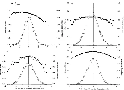
Form of apparent selection on a quantitative trait In a nonequilibrium population, we expect Wobs(X’)

for an additive trait to show directional selection; Figure 1A gives w o b s ( x ’ ) for an additive trait, at ran-

dom allele frequencies. We expect to observe stabilizing selection on an additive trait if the population is at a stable polymorphic equilibrium determined by selection. Figure 1, B-D, present the form of apparent

selection on a purely additive trait for the three viability models considered. Figure 2A represents

w o b s ( x ’ ) for a traits with random dominance. Figure

2B describes apparent selection on a trait with both random dominance and epistasis. This figure suggests that the conclusion about apparent stabilizing selection on additive traits with random dominance may be generalized for nonadditive traits with random epistasis.

In these figures, the average relative fitness per class wobs(x’) is almost perfectly quadratic, with its highest value at or very near

X.

This changes if the average of the dominance contributions is not zero, but now the fitness model as well as the trait compo- sition becomes important (Figure 2C). We observe directional, almost linear, selection if the coefficients of the trait are constant multipliers of the coefficients of fitness (Figure 2D). In other situations (G. DE JONC and S. GAVRILETS, unpublished results) we can observe very complex fitness functions with clearly asymmetric selection at low epistasis in the trait; at higher epistasis the maximum is displaced from

X.

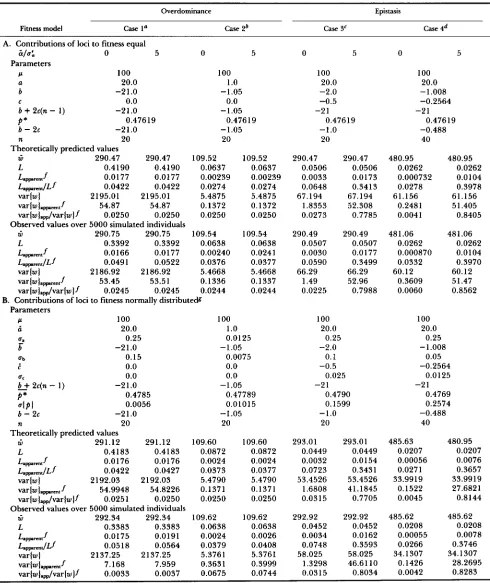
Strength of apparent selection on a quantitative trait: In Table 1, different characteristics of the real and apparent strength of selection in the additive model and in the epistatic model are given. In this table quantities from theoretical expectations arrived by summation over loci as in (10, 11) and (34) are listed together under the heading “Theoretical,” and quantities computed from a sample of 5000 individuals are listed together under the heading “Ob-

served.” T h e observed coefficient s was estimated by the regression of individual fitness w on the squared deviation of an individual’s trait value from the sample mean. T h e apparent load is estimated by sVg where V, is the phenotypic variance. This apparent load corresponds to Vg/2Vs in (BARTON 1990; KEIGHTLEY and HILL 1990). T h e observed fitness deviation for any individual can be divided into two independent parts, the deviation of w ( x ) from zi, and the deviation of w

from the apparent fitness w ( x ) : w

-

zi, = [ w ( x )

-

51

+

[w

-

w ( x ) ] . T h e total observed variance in fitness var(w),bS becomes the sum of var(w(x)

-

Zi)),bs and

var(w

-

w(x))obs. T h e quantity var(w)obs estimates the

variance in the real fitness, var(w), while the quantity var(w(x)

-

W)obs estimates var(w)app.

In Table 1, two cases for the overdominant fitness model and two cases for the epistatic fitness model are presented. T h e overdominant case 1 has the same average fitness and equilibrium allele frequencies as the epistatic case 3, while the overdominant case 2 has about the same total load as the epistatic case 3. Case

(10)

S. Gavrilets and G . de Jong

1.0 -

0.2 -

f

l

"

-4 -2 0 2 4

C

0.2.

-1.0

- 0.8

- 0.6

- 0.4

- 0.2

-

0.0

-1.0

- 0.8

C 0

-0.6

2

0.8 -

-

L c - V

0.4 - -0.4 E E

E!

0

-0.2

0.0

6 -4 -2 0 2 4

-1.0

- 0 8

0

=

.-

L

-0.6

+

. I

V -0.4

'

>

- 0 . 2

f

1.0-

D

0.8-

.

0.6.

c c '

5 0.4-

2

0.2-

0

m

I

_rp

0,"

0.0- P r P

.

0.0 ~ - Q l

-4 -2 0 2 4 -4 -2 0 4

0.0

Trait value x' in standard deviation units

2

Trait value x' in standard deviation units

FIGURE 1 .-Apparent selection on an additive trait pleiotropic to fitness. Shown are the apparent fitness as a function of trait value and the frequency distribution of trait values. The trait is determined according to expression (40), with:p = 0 , LU = 10.0, uz = 4.0,

3

= 0, ui =

0, i. = 0, ut = 0. (A) Nonequibbrium population, random allele frequencies. Epistatic asymmetric fitness model, expression (33), with m =

100, ci = 20.0, u: = 0.0625, b = -2.0, uz = 0.01, t = -0.5, u: = 0.000625. (B) Equilibrium population. Overdominant fitness model, expression 12, with m = 100, ci = 20.0, u: = 0.0625, i = -21.0, u; = 0.0225. (C) Equilibrium population. Symmetric fitness model, expression (39), 5 = 0.5; = 4.5. (D) Equilibrium population. Epistatic asymmetric fitness model, expression (33). with m = 100, i = 20.0, 6.'= 0.0625,

6

= -2.0, uz = 0.01, t = -0.5 and u? = 0.000625.

ing overdominant model. T h e ratio of the strength of apparent selection to the strength of overall selection is much higher in the epistatic model.

In the case of overdominance, the characteristics of the apparent selection do not depend upon the degree of "adaptivity," ie., on the relation between the mean and the variance of ai. In Figure 3, the ratio of apparent load to total load is given. In Figure 3, A and

B,

the equilibrium allele frequencies and the mean fitness are the same. If epistasis is absent, as in Figure 3A, no effect of the mean and the variance of the contributions of the loci to the trait is found at all. Without epistasis we find that both the explained part of the genetic load and the explained part of the genetic variance in fitness are very small (Table 1, case 1). In the epistatic model these values are small if a!

<<

u,, but become very large if a!

>>

u, (Figure

3B).

In Figure 3C, the explained part of the genetic load is given for different strength of epistasis, for both a!

<<

a, and a!

>>

ua. T h e apparent load at &

>>

a, is independent of the parameter c, only de- pendent upon b

+

2c(n

-

l), as shown in expression

(35).

At 6 / u a = 0, the intensity of selection is demon- strated by expression (37). T h e part of the genetic load explained by the apparent stabilizing selection

only appreciably rises with the strength of epistasis when the absolute value of 2c(n

-

1) is larger than the absolute value of 6 , at around c = -0.3.

This is illustrated in Figure

4,

A and B, by plotting the actual fitness of 100 individuals as well as their apparent fitness value on the basis of their trait value. As can be seen in Figure 4A, the overdominant model does not lead to a clustering of fitness values around

w ( x ) . In Figure

4B,

the degree of epistasis is high, and individual fitnesses follow the apparent fitness function almost perfectly. This is a visual example of the difference between the overdominant and epistatic models in explaining the genetic variance in fitness. T h e part of the genetic variance in fitness that is explained increases with the number of loci in the presence of high epistasis (Figure 4C). T h e epistatic model performs well in both the ratio of explained fitness variance to the total fitness variance, and the ratio of apparent load to total genetic load. T h e overdominant model cannot distinguish between "neutral" and "adaptive" traits.

DISCUSSION

(11)

Stabilizing Selection and Epistasis 619

0.4. -0.4

a

m

0.2-

e

-0.2

0 0

a

0.0,

-

,

-4 -2

Doob

I -n , 0.0

0 2 4

l.O- c

I

-1.0

0.8- I -0.8

0.2. -0.2

@

P ₀₀

o . om ” - B

m

OD0

-4 -2 0 2 4

0.0

Trait value x ’ in standard deviation units

c

e

0.6-

L

u

2

0.4-

z

-1.0

-0.8

E 3

-0.6

2

n

0

E

-0.4

s

‘y

U

- 0.2

1.0-

0.8 -

0.6-

c

E

u -

c

2 0.4-

2

-1.0

-0.8

c 0

L

-0.6 .-

’D t:

-0.4 y

a

?

E

U

0.2 - 8 O

m

- 0.2

0

W 0

9,

-8 -6 -4 -2 0 2 4

,o.o

Trait value x’ in standard deviation units

FIGURE 2.-Apparent selection on traits pleiotropic to fitness and influenced by dominance and epistasis. Shown are the apparent fitness as a function of trait value and the frequency distribution of trait values. Fitness in !he equilibrium populations is according to the epistatic asymmetric fitness model, expression (33), with m = 100, ci = 20.0, u: = 0.0625, b = -2.0, uf = 0.01, E = -0.5 and u: = 0.000625. (A) Random dominance, no epistasis in the trait: p = 0, 6 = 10.0, uq = 4.0,

s

= 0, uj = 9.0, i. = 0 and u: = 0. (B) Random dominance, random epistasis in the trait: p = 0, & = 10.0, uz = 4.0,

p

= 0, uz = 9.0, i. = 0 and u: = 0.25. (C) Partial dominance, no epistasis in the trait: p = 0,

d = 10.0, bp, = 7.0, = -4.0, u; = 0.0, i. = 0 and u: = 0. (D) Dominance and epistasis in the trait, averages of the trait coefficients a constant multiple of the averages of the fitness coefficients: p = 0, & = 10.0, uz = 16.0,s = -4.0, uj = 0.16, i. = -1.0 and u: = 0.025.

on a quantitative trait pleiotropically connected with fitness. For any polygenic system in which variability is maintained by selection, all we need is either that the trait be additive, or that dominance and epistatic effects of loci on the trait to be considered as independent random variables with mean zero. Such a consideration implies that the sign of the dominance and epistatic effects of the loci on the trait is random with respect to their effect on fitness. This “independence” of the allele effects of these two types can be naturally interpreted as “neutrality” of the allele effects on the trait. For a polygenic system in which a low level of variability is maintained by mutation or migration, an additional condition is that the additive effects are “neutral” too. On the other hand, in order to observe “directional” selection on a quantitative trait, either the genetic system has to be at a “tran- sient” state, or the effects of the loci on the trait have to be systematically related to those on fitness. T h e natural interpretation of the latter case is “adaptivity” of the corresponding contributions of the loci to the trait. Assuming that the genetic system is at a stable equilibrium determined by selection, we therefore can say that any quantitative trait for which nonadditive contributions are absent or random and independent

of those to fitness will exhibit “stabilizing selection,” while traits for which nonadditive contributions are related to those to fitness will exhibit “directional selection.” For genetic systems in which variability is maintained by mutation or migration, any trait for which both additive and nonadditive contributions are random and independent of those to fitness will be under apparent stabilizing selection and any trait with contributions related to those to fitness will be under apparent directional selection.

Two pleiotropic models with additive fitness were recently analyzed with respect to their utility to account for both the high heritability and the strong apparent stabilizing selection which are commonly observed: mutation-selection balance model (BARTON

(12)

620 S. Gavrilets and G. de Jong

TABLE 1

Comparison of overdominant and epistatic fitness model: effect of “neutral” and “adaptive” traits on apparent selection, apparent load and explained load, apparent fitness variance and explained fitness variance

Overdominance Epistasis

Fitness model Case la Case 2‘ Case 3‘ Case qd

A. Contributions of loci to fitness equal

&/ah 0 5 0 5 0 5 0 5

P 100 100 100 100

a 20.0 1

.o

20.0 20.0

b -21.0 -1.05 -2.0 -1.008

C 0.0 0.0 -0.5 -0.2564

b

+

2c(n

-

1) -21.0 -1.05 -2 1 -21

b

-

2c -21.0

-

1.05 -1.0 -0.488

n 20 20 20 40

ri, 290.47 290.47 109.52 109.52 290.47 290.47 480.95 480.95

L 0.4 190 0.4190 0.0637 0.0637 0.0506 0.0506 0.0262 0.0262 L.ppsmntf 0.0177 0.0177 0.00239 0.00239 0.0033 0.0173 0.000732 0.0 104 L,-,/L~ 0.0422 0.0422 0.0274 0.0274 0.0648 0.3413 0.0278 0.3978 var(w) 2195.01 2195.01 5.4875 5.4875 67.194 67.194 61.156 61.156 varIwtaWmntf 54.87 54.87 0.1372 0.1372 1.8353 52.308 0.2481 5 1.405 var(w),/var(w)f 0.0250 0.0250 0.0250 0.0250 0.0273 0.7785 0.0041 0.8405

ri, 290.75 290.75 109.54 109.54 290.49 290.49 481.06 48 1.06

L 0.3392 0.3392 0.0638 0.0638 0.0507 0.0507 0.0262 0.0262

Parameters

P* 0.47619 0.476 19 0.47619 0.47619

Theoretically predicted values

Observed values over 5000 simulated individuals

L p p W “ t f 0.0166 0.0177 0.00240 0.0241 0.0030 0.0177 0.000870 0.0104

L.,.JL~ 0.049 1 0.0522 0.0376 0.0377 0.0590 0.3499 0.0332 0.3970 varlw) 2186.92 2186.92 5.4668 5.4668 66.29 66.29 60.12 60.12 varlwt.,,tf 53.45 53.51 0.1336 0.1 337 1.49 52.96 0.3609 51.47 var(w).pp/var(w)f 0.0245 0.0245 0.0244 0.0244 0.0225 0.7988 0.0060 0.8562

B. Contributions of loci to fitness normally distribute& Parameters

P 100 100 100 100

ci 20.0 1

.o

20.0 20.0

0, 0.25 0.0125 0.25 0.25

b -2 1

.o

-1.05 -2.0

-

1.008

E 0.0 0.0 -0.5 -0.2564

UC 0.0 0.0 0.025 0.0125

-

b

+

2c(n

-

1) -21.0 -1.05 -2 1 -2 1

P* 0.4785 0.47789 0.4790 0.4769

U l P t 0.0056 0.01015 0.1599 0.2574

ob 0.15 0.0075 0.1 0.05

b

-

2c -21.0 -1.05 -1.0 -0.488

n 20 20 20 40

ri, 291.12 291.12 109.60 109.60 293.01 293.01 485.63 480.95

L 0.4183 0.4183 0.0872 0.0872 0.0449 0.0449 0.0207 0.0207

Lspp.mtf 0.0 176 0.0176 0.0024 0.0024 0.0032 0.0 154 0.00056 0.0076 L.,,JL~ 0.0422 0.0427 0.0373 0.0377 0.0723 0.3431 0.0271 0.3657 varlw) 2192.03 2192.03 5.4790 5.4790 53.4526 53.4526 33.9919 33.9919

var Iw

t

pWWnt f 54.9948 54.8226 0.1371 0.1371 1.6808 41.1845 0.1522 27.6821

var(wIapp/var(wIf 0.0251 0.0250 0.0250 0.0250 0.03 15 0.7705 0.0045 0.8144

ri, 292.34 292.34 109.62 109.62 292.92 292.92 485.62 485.62

L 0.3383 0.3383 0.0638 0.0638 0.0452 0.0452 0.0208 0.0208

Theoretically predicted values

Observed values over 5000 simulated individuals

Lappsrmtf 0.0175 0.0191 0.0024 0.0026 0.0034 0.0162 0.00055 0.0078 LspPs-1/Lf 0.0518 0.0564 0.0379 0.0408 0.0748 0.3593 0.0266 0.3746 var(w

1

2137.25 2137.25 5.3761 5.3761 58.025 58.025 34.1307 34.1307 varIwlappnntf 7.168 7.959 0.3631 0.3999 1.3298 46.6110 0.1426 28.2695 var(w),/var(w)f 0.0033 0.0037 0.0675 0.0744 0.03 15 0.8034 0.0042 0.8283

Case 1 and case 3 have similar mean fitness ri, but differ in epistasis c.

Case 2 and case 3 have approximately similar genetic load L but differ in epistasis c. Cases 1, 3 and 4 have identical nonadditivity b

+

2c(n - 1).

Case 3 and case 4 differ in number of loci n.

e &/ua = 0 stands for a “neutral” trait; %/urn = 5 stands for an “adaptive” trait. f “Neutral” us. “adaptive” has an influence only under the epistatic fitness model.

Pleiotropic models of polygenic variation, stabilizing selection, and epistasis.