R E S E A R C H
Open Access
The use of cognitive ability measures as
explanatory variables in regression analysis
Brian Junker
1, Lynne Steuerle Schofield
2and Lowell J Taylor
3**Correspondence: [email protected] 3Heinz College, Carnegie Mellon University, 5000 Forbes Avenue, Pittsburgh, PA 15213 Full list of author information is available at the end of the article
Abstract
Cognitive ability measures are often taken as explanatory variables in regression analysis, e.g., as a factor affecting a market outcome such as an individual’s wage, or a decision such as an individual’s education acquisition. Cognitive ability is a latent construct; its true value is unobserved. Nonetheless, researchers often assume that a test score, constructed via standard psychometric practice from individuals’ responses to test items, can be safely used in regression analysis. We examine problems that can arise, and suggest that an alternative approach, a “mixed effects structural equations” (MESE) model, may be more appropriate in many circumstances.
JEL Code: J01
Keywords: Labor economics, Structural equations modeling, Item response theory
1 Introduction
Cognitive test scores—whether from standardized achievement tests or from cogni-tive items on surveys—are used widely as explanatory or control variables in the social sciences.1Political scientists use cognitive test scores as a descriptive demographic vari-able to characterize voting behavior (Venezky and Kaplan 1998). Health researchers are interested in how cognitive ability (and other latent constructs, e.g., depression) affects a patient’s understanding of and likelihood of following prescribed therapies (Schillinger et al. 2002). Social scientists control for “ability” in analyses that seek to evaluate the role of parental financial resources in determining post-secondary education (Dynarski 2002).
The analyses in such studies often proceed using linear regression models, such as
yi=β0+β1θi+β2Zi+β3Wi+εi, (1)
where yi is an outcome for individuali,θi is a measure of the latent construct from a test,Ziindicates the contrast of central interest, andWirepresents other covariates. For example, equation (1) has been used extensively in labor economics—in analyses intended to tease apart the influences of cognitive ability (as measured byθi) and possible market effects of race or gender status (Zi) on log wage(yi). Prominent examples include Neal and Johnson (1996), Bollinger (2003), and Lang and Manove (2011).
The variableZiis typically a 0/1 indicator for two groups. In the case of designed exper-iments (or natural quasi-experexper-iments), the groups are treatmentvs.control; in the case of observational studies that examine disparate outcomes for some specific group (e.g.,
a racial or ethnic group), we might refer to groups asfocalvs. reference(Holland and Thayer 1988; Penfield and Camilli 2007). In a study of wage disparities between reference and focal groups, for example,β1is the “return to cognitive ability,” andβ2is intended to measure disparate treatment in the labor market for members of the focal group.
A key obstacle to obtaining (asymptotically) unbiased estimates ofβ1andβ2in (1) is
the possibility of measurement error inθi. Indeed, standard theory for scoring cognitive tests (Lord and Novick 1968) takes as axiomatic thatθiis a latent variable, and any proxy for it entails some measurement error. It is well known that regression coefficients are biased if measurement error is ignored. Standard approaches for dealing with this sort of measurement error include the use of nonparametric bounds, instrumental variable estimation, and direct modeling.
Nonparametric bounds are invaluable, especially when little is known about the data-generating process. For example, Bollinger (2003) shows that failing to correct for measurement error in (1) can lead the researcher to estimate a black-white wage differ-ence that is biased downward, and calculates Klepper and Leamer (1984) bounds for the regression coefficients. Such nonparametric bounds can be wide. In Bollinger’s empirical example, which studies the impact of race on log wage (the focal group is black and the reference group is white), the estimated bounds for men are (−0.07, 1.26) and for women are (0.04, 1.39).2
Instrumental variable methods provide a standard answer to measurement error in a regressor when instruments of sufficient quality and relevance can be found. However, the measurement error in cognitive test scores is itself exogenous; it is dependent only upon the measurement procedure in a well-designed test, and not on omitted variables that might be associated with any outcome of interest. Thus instrumental variables will typically not be of use in correcting for it. In cases where instruments can be found, one would expect them to be rather weak (leading to problems discussed in Staiger and Stock (1997)).
Whenθi is to be obtained from a well-constructed cognitive assessment using stan-dard modern technology (such as the assessments listed in footnote a), a direct model for measurement error has already been used as part of the quality-control process of con-structing the test, and is available to produce scoresθiwith known measurement error properties. The class of models used to construct many standard cognitive assessments is known as item response theory (IRT) models (van der Linden and Hambleton 1997).
The existence of IRT as a direct model obviates the need for refining nonparametric bounds or searching for suitable instruments to adjust for measurement error in cognitive test scores. Indeed, because the cognitive assessment wasconstructedto fit this model, answers obtained using this model have more authority than answers using other meth-ods, regardless of raw comparisons of effect size estimates, statistical significance, etc. The class of IRT models is flexible enough that it should be considered as a direct model for measurement error even in cases in which number-correct score might be used, even if the test was not constructed using IRT techniques.
the lines of equation (1). Third, we illustrate the methodology in two applications, one linear and one non-linear.
We note finally that our work is focused on a particular kind of error in a particu-lar kind of variable in errors-in-variables regressions such as equation (1): measurement error inherent in psychometric measures of cognitive status. We have nothing to add here about problems that emerge due to other variables being measured with error, e.g., self-reported years of schooling, parents’ schooling, parents’ income, etc.
2 Models used to construct cognitive test scores
Well-constructed cognitive tests use statistical methodology as a quality control device in the construction of the test. The process inevitably involves the interplay of defining and refining the construct to be measured, designing test items to measure it, defining a space of responses and scoring rules for each possible response in the space, and finally developing a statistical measurement model to assemble responses to test items into an observed “score” that measures the construct with some quantifiable level of error (e.g., Wilson 2005). Candidate test items that do not produce data consistent with the measure-ment model are rejected in favor of those that do; in this sense, the data from a well-built cognitive test fits the statistical measurement modelby construction.
Some cognitive assessments—especially ones intended for smaller-scale use—are built using a measurement model calledclassical true-score theory(CTT). Under this model the observed test scoreXiis expressed in terms of a true score (or latent cognitive status)
θiand measurement errorνi,
Xi=θi+νi. (2)
This model, together with standard distributional assumptions, has been useful for thinking about measurement errorνi whenXiis the total score (number-correct score). For example, standard psychometric formulae such as the Spearman-Brown formula for expressing the reliability of a total score as a function of test length, or Cronbach’s alpha lower-bound for reliability—are based on elaborations of CTT (see Lord and Novick 1968).
More commonly, especially for large-scale assessments or for cognitive portions of large-scale surveys, the measurement model used to build the test is anitem response theory(IRT) model. IRT models can be thought of as a generalization of mixed effects logistic regression models (Stiratelli et al. 1984). Instead of modeling the total scoreXifor individuali, IRT models focus on the individual responsesXijof individualito test itemj. One of the most common IRT models in cognitive testing is thethree-parameter logistic
(3PL) model. LettingXij=0 for an incorrect answer andXij=1 for a correct answer, the 3PL model posits the probability of a correct response as
Pj(θi)≡P[Xij=1]=cj+
1−cj 1+exp[aj(θi−bj)]
, (3)
is the probability thatXij=1. The parametercjis a “guessing parameter” measuring the likelihood that a very low-ability examinee would respond correctly simply by guessing. The parameterajmeasures how influential changes inθiare on changes inP[Xij = 1], and conversely, drives the level of measurement error. Sijtsma and Junker (2006) give a brief overview of CTT, IRT and related models; Rao and Sinharay (2007) provide more in-depth reviews.
2.1 Measurement error in IRT models
Measurement error in IRT models can be thought of as the standard error of estimation forθi from the pattern of scored item responses from examineei(van der Linden and Hambleton 1997). For example, conditional on knowing the item parametersaj,bjand
cj, the likelihood for a particular pattern of wrong and right answers on a test ofJitems following the 3PL model is
P[Xi1=xi1,. . .,XiJ=xiJ|θj]= J
j=1
Pj(θi)xij(1−Pj(θi))1−xij,
from which it is straightforward to calculate that the Fisher information for estimatingθi
is
I(θi)= J
j=1
[Pj(θi)]2
Pj(θi)(1−Pj(θi))
; (4)
the measurement error is thenSE(θi)=1/√I(θi).
This immediately suggests that the IRT model imposes some constraints on the mag-nitude of the measurement error forθi. Indeed, taking the simplest case, if allaj=1 and
bj=cj=0, then
SE(θi)=
1
√
J
1+eθi eθi/2
. (5)
While in principleθi may be any real number, as a practical matter anyθi less than roughly−4 is indistinguishable in data from any other; and similarly for anyθi greater than roughly+4. The first panel of Figure 1 depicts the measurement error curve for equation (5) over the range−4≤θ ≤4, for a test of lengthJ=20 items; the other three panels illustrate the measurement error for more typical 3PL tests. (See Schofield (2008) for additional discussion.)
Such a precise specification of measurement error might normally be rejected as reflecting unacceptably strong modeling assumptions. In this case, however, the strong assumptions are not being made by the analyst but rather are guaranteed by the construc-tor of the test. Even in cases where the test was not constructed explicitly with IRT in mind, IRT models can fit well and provide strong information about measurement error. It would be foolish not to use these assumptions to the fullest extent, since they are available to us by construction.
2.2 Estimation in IRT models
-4 -2 0 2 4
0.0
1.0
2.0
3.0
(a)
SE(
)
-4 -2 0 2 4
0.0
1.0
2.0
3.0
(b)
SE(
)
-4 -2 0 2 4
0.0
1.0
2.0
3.0
(c)
SE(
)
-4 -2 0 2 4
0.0
1.0
2.0
3.0
(d)
SE(
)
Figure 1 Measurement error under IRT models:(a)for the simple model whose measurement error is expressed in equation (5);(b),(c),(d)for more typical 3PL tests of length 20, 40 and 80 items. (a)Measurement error for simple model, J=20,(b)Measurement error for typical 3PL, J=20,
(c)Measurement error for typical 3PL, J=40,(d)Measurement error for typical 3PL, J=80.
Sinceθi is a random effect it is typical to assumeθi is iid Normal, with mean 0 and varianceτ2to be estimated. This leads to the marginal likelihood forNexaminees andJ
items,
L(a1,. . .,aJ,b1,. . .,bJ,c1,. . .,cJ,τ2)= N
i=1
J
j=1
Pj(θi)xij(1−Pj(θi))1−xijn(θj|μ,τ2), (6)
whereμ=0 is assumed, and all other parameters are to be estimated. In some situations theμ= 0 assumption and even the simple normality assumption may be relaxed, as in the next Section, for example.
Thea,b,candτ2parameters may be estimated from equation 6 using direct maximum likelihood, an E-M algorithm, or Bayesian methods (after endowing all of the parameters with suitable prior distributions). In practice there is little difference between ML and Bayesian estimates for these models (Fox 2010). Because of this, and because of its conve-nience for constructing and estimating hybrid models, we focus on Bayesian estimation for the remainder of the paper.
3 Accounting for cognitive score measurement error
In order to useθiin an analysis like that of equation (1), we must either (a) combine the IRT model with the regression model to estimate coefficients in (1) directly, or (b) provide estimates or imputations for eachθi that incorporate suitable measurement error into equation (1). We consider each method in turn.
3.1 Joint modeling to account for cognitive score measurement error
Schofield (2008) sets out a mixed effects structural equations (MESE) model, which we employ here for the problem of adjusting our key regression (1) when we replaceθ with a fallible test score.3The latent cognitive variable is a random effect and the IRT and linear model parameters are all fixed effects, so this is a “mixed effects” model.
Mislevy (1991) shows, in the context of estimating subpopulation parameters for the National Assessment of Educational Progress (NAEP) and similar large-scale surveys, that incorporating latent variables from a measurement model into a regression analy-sis requires more elaborate random-effects distribution forθithan shown in equation 6 above. Instead of assumingμ=0 in then(θ|μ,τ2)density shown there, we must assume thatμ=α0+α1Zi+α2Wi(withα0,α1andα2to be estimated). The need for this more
elaborate conditioning is also discussed by Schofield et al. (2012). Thus, for equation (1) the MESE model takes the form
yi|Zi,Wi,θi ∼ N(β0+β1θi+β2Zi+β3Wi,σ2) (7)
xij|θi ∼ IRT(xij|θi,γj) (8)
θi|Zi,Wi ∼ n(θi|α0+α1Zi+α2Wi,τ2) (9) where θi, Zi, Wi and yi have the same roles as in (1) and IRT(xij|θi,γj) is a suitable IRT model with parametersγjfor each itemj(e.g., for the 3PL model,γj ≡ (aj,bj,cj)). Equation (7) corresponds to equation (1), and is the regression of primary substantive interest.
Equation (7) is easily modified to accommodate logistic regression, or any other gen-eralized linear model. In the case of logistic regression,yibecomes an indicator variable and equation (7) becomes
yi ∼ Bernoulli(pi) log pi
1−pi = β0+β1θi+β2Zi+β3Wi
. (10)
The MESE model solves some of the known identification problems often associated with errors-in-variables models. Typically, errors-in-variables models cannot be identi-fied unless there is additional data in one of three areas: (1) replicate measures ofXi, the observed test score, (2) distribution information onθi, the unknown true score, or (3) distributional or moment restrictions on the error distribution (Stefanski 2000). By embedding the IRT model into the MESE model, we exploit the IRT model to provide further information about the measurement error of the cognitive test score.
As for identification of the IRT model itself, the location and scale parameters of the latent distribution are confounded with the difficulty and discrimination parameters of the measurement model. In the 3-PL model, for example, the scales ofbjandθiare iden-tified only up to an additive constant and the scales ofajand bothθiandbjare identified only up to a multiplicative constant. This indeterminacy of the IRT scales has ramifica-tions for the regression coefficients; the choice of the latent scale ofθiaffects the scale of
ˆ
β1. This choice does not affect statistical tests for the significance ofβˆ1, nor does it affect
estimated coefficients for other covariates (Schofield 2008).
The indeterminacy of the IRT scales is easily dealt with, by fixing the scale ofθ (e.g.,
μθ =0 andσθ=1.) Even when the item parameters are unknown and must also be
esti-mated, there are well-known estimation methods (e.g, Bayesian MCMC, Patz and Junker 1999) to appropriately fix the scale ofθ and the item parameters to ensure that the model is identified.4
As discussed below, in many empirical applications in economics analysts simply sub-stitute a test score into regressions such as (7), thereby ignoring variation inherent in the measurement of cognitive ability. Exceptions include important recent work by James Heckman and co-authors: Hansen et al. (2004) and Cunha and Heckman (2008), for example, extend classical test-score models (Lord and Novick 1968) and the subsequent MIMIC approach (Joreskog and Goldberger 1975), which deals with measurement issues for posited latent variables when there are multiple observed indicators.5These papers
provide a template for the treatment of latent variables in applications for which multi-ple measures are available—usually a small number of measures. As we have noted, the MESE approach uses this same logic, but we are working with a case in which a typically larger number of replicate measures (generally “item responses”) are available, and those measures take a form that is appropriately handled by an embedded IRT model.
3.2 Multiple imputation to account for cognitive score measurement error
Starting with the U.S. National Assessment of Educational Progress (NAEP) in the 1980’s (as reviewed by Mislevy et al. 1992), many large scale educational surveys release multiple
plausible values(PVs)—known in the statistics literature asmultiple imputations(Rubin 1987)—for each examinee’s proficiency, rather than a single proficiency estimate. PVs are draws from a posterior distribution ofθifor individuali, given that individual’s responses to items on a test and a set of background characteristics in a “conditioning model.” Typ-ically, agencies release five PVs for each individual, and secondary analysts are instructed in the use of PVs for estimating statistics.
PVs solve three related problems for these agencies: (1) by law, certain government sur-veys such as NAEP are proscribed from releasing individual test scores to the general public, and PVs provide a potential way of protecting individual confidentiality; (2) many more test questions are used by these surveys than one examinee can respond to, and PVs provide for comparison on a common scale regardless of the difficulty of the questions asked; and (e:3pl) PVs are constructed to represent the uncertainty (measurement error) inherent in using a finite number of tasks or test questions to measure an unobservable latent construct such as literacy or math proficiency.
When a well-constructed ensemble of PVs is used in accordance with their construction (e.g., Mislevy 1991 and 1993, and Li et al. 2009) in a secondary analysis, biases due to mea-surement error in cognitive score are negligible. Indeed, the posterior distribution from which plausible values are drawn is typically given by a model similar to that of equations (8) and (9) alone, withZandWenlarged to include (proxies for) all possible regressors or contrasts that a secondary analyst might use.7Except for the larger conditioning model forθ, correct use of PVs in (1) is in essence the same as estimating coefficients in (1) using MCMC methodology based on the MESE model.
There are three practical problems with PV methodology. First, there are only a few national and international surveys with the resources to produce PVs for secondary ana-lysts. Second, PVs released by survey agencies involve θs conditioned on many more variables than are needed in any particular secondary analysis, and can create additional problems (Schofield et al. 2012). Third, secondary analysts may be tempted to sidestep the correct procedure for using PVs as outlined by Mislevy (1991) and others. For exam-ple, in their study of international comparisons of wage inequality, Blau and Kahn (2005) treat the means and medians of individuals’ PVs in the 1994–96 International Adult Literacy Survey (IALS; Murray et al. 1997) as iftheywere the accurately measured levels of cognitive skills. von Davier et al. (2009) argue that this undermines the bias-correction built into PVs.
4 Applications in labor economics
4.1 Analyzing racial disparity in labor market outcomes
Several applications of equation (1) are found in labor economics. In this context the data is usually observational, from surveys such as the 1979 National Longitudinal Study of Youth (NLSY79; Zagorsky et al. 1997) or 1992 National Adult Literacy Survey (NALS; Kirsch et al. 2000), the outcome yi is a market outcome or individual choice (e.g., log wage, labor force participation, or educational attainment),Ziis an indicator of reference (Zi=0) vs. focal (Zi=1) group (e.g., white vs. black),θiis a cognitive test score, andWi are any other relevant explanatory variables.
Neal and Johnson (1996) provide a landmark example. In that study the authors evaluate the role of cognitive skills acquired by youth (prior to entry in the labor market) on subse-quent wage outcomes in U.S. labor markets. Using data from the NLSY79—which include individuals’ scores the Armed Forces Qualifying Test (AFQT)—the authors show that most of the black-white wage gap can be traced back to cognitive skills differentials that emerge at young ages.
Another example is Ritter and Taylor’s (2011) examination of racial differences in unem-ployment, using the same data and same basic approach as Neal and Johnson (1996). They find that black individuals have substantially higher levels of unemployment over their work careers than their white counterparts, and show further that much of this gap remains after accounting for racial differences in cognitive skills as measured by the AFQT.
education, and, consistent with the posited theory, they find that among individuals with similar cognitive skills, black men and women are more likely than their white counterparts to pursue higher education.
In each of the examples listed above, a cognitive test score is used as an explanatory variable, rather than treated as a latent construct. The hope presumably is that bias intro-duced is not too large. At the present time, items response data are not available for the AFQT for NLSY79 respondents, so it is not possible to assess empirically how problem-atic errors-in-variables bias might be in the specific applications listed above. Instead, in our analyses below we use data from similar sources, for which we do have item response data.
4.2 Black-white wage differences in the U.S.
To illustrate the two direct modeling approaches for dealing with the measurement error inherent in cognitive test scores—the MESE model and the use of PVs—we begin with an example that uses data from the NALS. These data include an individually-administered household survey of 24,944 adults aged 16 and over. The NALS is comprised of two sets of questions: standard demographic questions (race, gender, labor force behavior, mari-tal status, education, etc.) and cognitive items that measure functional literacy in three domains: prose, document, and quantitative. The NALS was designed with 165 items to test the literacy skills of examinees, but each examinee was administered a representative sub-sample of approximately one-third of the full set of 165 items. Items not answered are treated as missing at random in the analyses below, as is common practice for designed missingness due to fractional designs and the like.
Our focus in our example is on racial differences in log wages. Table 1 provides some demographic characteristics of the NALS sample for blacks and whites. Three features merit attention. First, on average white men earn more than black men and white women earn more than black women. Second, on average black adults have relatively less educa-tion. Third, literacy skills, as measured by mean of plausible values, are relatively lower
Table 1 Sample characteristics, 1992 National Adult Literacy Survey (NALS)
Black men Black women White men White women
N 1665 2807 7449 9404
Average Age 39.4 39.4 40.5 42.4
Marital Status
Proportion never Married 0.39 0.38 0.28 0.19
Education
Proportion Still in HS 0.06 0.04 0.04 0.03
Proportion<HS 0.29 0.29 0.13 0.14
Proportion HS 0.29 0.29 0.27 0.30
Proportion<College 0.25 0.29 0.30 0.33
Proportion College + 0.11 0.09 0.26 0.21
Literacy Skills
MeanPlausible Value -0.66 -0.50 0.48 0.50
St. Dev.Plausible Value 1.14 1.18 1.03 0.96
Earnings of Full-Time Workers
Average Weekly Wage 452.3 397.5 674.6 440.9
for black individuals than white individuals. NALS public-use data files from the National Center for Education Statistics (NCES) contain only basic data elements; in order to access individual cognitive item responses necessary for the IRT and MESE models, we also obtained restricted-use files from NCES.
We restrict our attention to just two subsets of the full NALS data set: men, mar-ried or single, aged 25–55, who work full time (work at least 35 hours for pay or profit during the week of their interview, either in one full-time job or in two or more part-time jobs), who report wages, and who answered at least one literacy item; and never marriedwomenwho meet the same age, work and reporting criteria. The two groups are fitted separately because labor market outcomes might differ for men and women. Mar-ried women are excluded from our analyses because of the difficulty of establishing their work experience.8
Our interest is the comparison of estimated coefficients when we ignore measurement error in the literacy measure (i.e., the “unadjusted” case) and when we make appropriate “adjustments” using the MESE model, i.e., equations (7)–(9). The NALS data also contains
M=5 plausible values per content area and individual, constructed using the methods outlined above. This allows us to also compare estimates when we make appropriate use of PVs.
In all of the analyses reported here,yiis the log of self-reported weekly wage,Zi =1 if the individual identifies as black (andZi=0 if white), andWiis a vector containing three covariates: “potential experience” (current age minus years of schooling minus 6) entered as a quartic, urban/rural status (a binary indicator), and census region (an unordered factor). For unadjusted analyses,θi is replaced with an IRT-based ML estimate of total score on the entire 165 item pool.9For adjusted analyses using the MESE model,θi is merely the latent variable that links equations (8) and (9). For adjusted analyses using PVs, the model (1) is fitted five times, once for each set of PVs, and the results are combined using the using jackknife method recommended by Mislevy et al. (1992).
Both the unadjusted and adjusted models were estimated using Bayesian methods, in particular using an MCMC algorithm specified in WinBUGS. This was done to enhance comparability of estimates across models. Model fit for all models was compared using the DIC fit statistic from WinBUGS (Spiegelhalter et al. 2002). All parameters are estimated, except for item parameters in the IRT model.10
For the unadjusted model involving only equation (7), we used flatN(0, 10000)priors on eachβ coefficient, and a Unif(0, 1000) prior on σ2. Bayesian estimates with these priors are extremely similar to OLS estimates.11 For the full MESE model, we used the same priors on theβ’s andσ2in (7), and we fixed the item parameters to their NCES-estimated values in (8). In (9) we use an inverse-Gamma(1,1) prior onτ, and we assume flat N(0, 100) priors on each α coefficient. In order to further set the scale of θ, we mean-centered each of the covariates in (9). These priors onθi allow for the possibil-ity that blacks and whites, and people of different experience levels, census regions, and urban/rural status, have different distributions of proficiency.
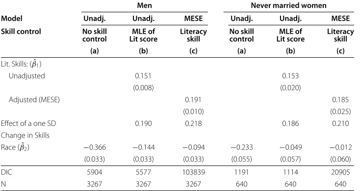
Table 2 Log wage regressions
Men Never married women
Model Unadj. Unadj. MESE Unadj. Unadj. MESE
Skill control No skill MLE of Literacy No skill MLE of Literacy
control Lit score skill control Lit score skill
(a) (b) (c) (a) (b) (c)
Lit. Skills: (βˆ1)
Unadjusted 0.151 0.153
(0.008) (0.020)
Adjusted (MESE) 0.191 0.185
(0.010) (0.025)
Effect of a one SD 0.190 0.218 0.186 0.210
Change in Skills
Race (βˆ2) −0.366 −0.144 −0.094 −0.233 −0.049 −0.012 (0.033) (0.033) (0.033) (0.055) (0.057) (0.060)
DIC 5904 5577 103839 1191 1114 20905
N 3267 3267 3267 640 640 640
Notes: Data are from the 1992 NALS, restricted to individuals aged 25–55 who work fulltime, reported wages, and who answered at least one literacy item. Unadjusted regressions employ the wage equation (1) with either no cognitive measure (column a) or a measure unadjusted for measurement error (column b). Column (c) provides estimates from the MESE model, equations (7)–(9), adjusting for measurement error in the cognitive measure. All regressions also control for potential experience entered as a quartic, census region (entered as dummy variables), and urban setting (entered as a dummy variable).
Standard arguments (Schofield 2008) suggest that if we ignore the errors-in-variables problem, we are likely to bias estimates ofβ1toward zero, and more importantly for our
purposes, bias estimates ofβ2downward. With this in mind, consider first our estimates ofβ1. Coefficients reported in columns (b) and (c) are not directly comparable, since they depend on the scale of the cognitive measure. A better comparison can be made by examining the estimated effect of an increase in skills equal to one standard deviation (as measured using the white population). For men this is seen to be 0.190 under the unadjusted model (column (b)) and 0.218 under the adjusted model (column (c)). Results are similar for women. In short, we observe the attenuation bias in the expected direction in the (b) columns.
More importantly, we see that for both men and women, failure to account appropri-ately for the latent structure of cognitive ability leads to bias in estimates of the effect of race in our wage regression. As expected, estimates ofβ2are biased downward in the
unadjusted cases.
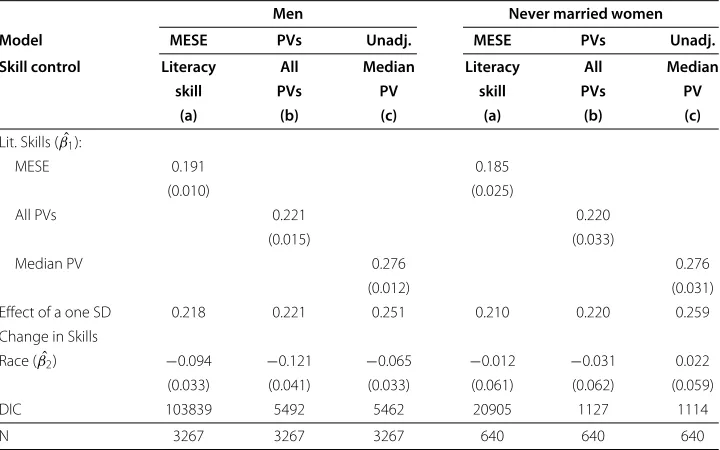
As discussed above, a defensible alternative approach to estimating equation (1) entails the appropriate use of plausible values (PVs), the multiple imputations of cognitive scores provided by some survey agencies in large scale surveys such as NALS. In Table 3 we compare wage-equation estimates from our MESE model, with two possible approaches for using plausible values (PVs). Columns (a) repeat our results for the MESE model from Table 2; columns (b) report results using the five sets of PVs provided by NCES with the NALS data set, combined using the procedure outlined in the Section entitled, Multiple imputation to account for cognitive score measurement error; and columns (c) report the result of using median PVs as a regressor in the wage equation (1). von Davier et al. (2009) provide formal arguments and Schofield (2008) provides informal arguments about potential biases for this sort of procedure–upward bias in the estimates of bothβ1
Table 3 Plausible-values adjustments for log wage regressions
Men Never married women
Model MESE PVs Unadj. MESE PVs Unadj.
Skill control Literacy All Median Literacy All Median
skill PVs PV skill PVs PV
(a) (b) (c) (a) (b) (c)
Lit. Skills (βˆ1):
MESE 0.191 0.185
(0.010) (0.025)
All PVs 0.221 0.220
(0.015) (0.033)
Median PV 0.276 0.276
(0.012) (0.031)
Effect of a one SD 0.218 0.221 0.251 0.210 0.220 0.259
Change in Skills
Race (βˆ2) −0.094 −0.121 −0.065 −0.012 −0.031 0.022 (0.033) (0.041) (0.033) (0.061) (0.062) (0.059)
DIC 103839 5492 5462 20905 1127 1114
N 3267 3267 3267 640 640 640
Notes: Data are from the 1992 NALS, restricted to individuals aged 25–55 who work fulltime, reported wages, and who answered at least one literacy item. MESE model estimates (column a) are from Table 2. “All PV’s” estimates (column b) employ the recommended procedure (Mislevy et al. 1992) for combining regression results for multiple imputations. “Unadjusted Median PV” estimates (column c) employ the median PV in the wage equation (1), with no adjustment for measurement error. All regressions also control for potential experience entered as a quartic, census region (entered as dummy variables), and urban setting (entered as a dummy variable).
In Table 3, as in Table 2, estimates of return to skills (β1) are not directly comparable,
because of scale dependence. However, estimates of the effect of a one SD increase in skills are very similar in columns (a) and (b), but somewhat inflated in columns (c), as expected given arguments in von Davier et al. (2009). Similarly, for both men and women,βˆ2is
reasonably similar in columns (a) and (b), but appears biased upward in the (c) columns. As discussed in the preceding Sections of our paper, either of the estimation procedures in columns (a) or (b) of Table 3 are defensible. The MESE model used in column (a) is designed to take full advantage of the direct model for measurement error that comes with NALS, and the PV method in column (b) duplicates this approach, using multiple impu-tations designed for secondary users. Numerical differences between columns (a) and (b) are small, and can be attributed to differences in the “conditioning model” expressed in equation (9): in our MESE model, only variables used in the wage equation were included in the conditioning, whereas for PVs, equation (9) is expanded to condition on (proxies for) all possible regressors and interactions that secondary analysts might use. For more details on differences one might expect to see with different conditioning models in (9), see Schofield et al. (2012).
The primary message from our empirical exercise is that the use of a “cognitive ability measure” as an error-free independent variable in a wage regression can lead to quite different inferences than a more defensible approach (MESE) that treats cognitive ability as a latent construct. For example, for men the estimated portion of the black-white log wage gap that is “unexplained” once we control for ability is−0.09 in our MESE model, which is more than one third smaller than the−0.14 estimate we get when we use the ML estimate of cognitive ability as a regressor. Our estimate also differs substantially from the
It is important to note that our estimates rely on a contemporaneous measures of skills, which is the consequence of skills development when individuals are young, which could be shaped by disparate pre-market treatment,andskills development among indi-viduals over time, which could be shaped in part by disparate treatment in the labor market. Our results are not directly comparable to those of Neal and Johnson (1996), for example. Although the regression framework is similar, conceptually their study is quite different: they use a measure of cognitive skills taken when individuals are quite young (still teenagers)—prior to their completion of school and entry into the labor market. Thus, their regression conceptually allows an assessment of the role of racial disparities ofpre-markethuman capital development on eventual labor market outcomes. Our esti-mates might be of independent interest; for example Ferrer et al. (2006), Murnane et al. (1995), and Blau and Kahn (2005) all use contemporaneous measures of literacy skills in analyses of various sorts.
4.3 The Black-white educational attainment gap in the U.S.
Lang and Manove (2011) recently investigated the possibility that education is a gen-erally more valuable signal of productivity for blacks that it is for whites. If so, their model predicts that young black individuals will invest more heavily in education than comparably-skilled whites. Evidence in support of this prediction comes from regressions that use data from the 1979 National Longitudinal Survey of Youth (NLSY79). In their regressions “educational attainment” is the dependent variable, and explanatory variables include a race indicator variable and a measure of cognitive ability (the AFQT). For most levels of the AFQT score, black men are found to have higher educational attainment than similarly skilled white men, and the same is true for women.
We estimate a similar regression to Lang and Manove (2011) using a different data source, the 1997 National Longitudinal Survey of Youth (NLSY97).13 This survey follows 8,894 youth born between 1980 and 1984. At the time of their first inter-view, individuals were aged 12-18. Since 1997, surveys have been conducted every year with data gathered on education attainment and enrollment, race, gender, and many other demographic items. Additionally, respondents have taken a standard skills assessment, the Peabody Individual Achievement Test-Revised mathematics assessment (PIAT; Markwardt 1998). We are therefore examining the determinants of the attain-ment of higher education for a more recent cohort than in Lang and Manove’s (2011) analysis.
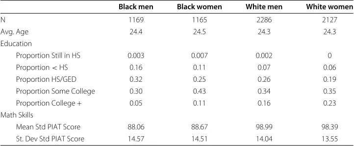
Table 4 Sample characteristics, National Longitudinal Study of Youth 1997 (NLSY97)
Black men Black women White men White women
N 1169 1165 2286 2127
Avg. Age 24.4 24.5 24.3 24.3
Education
Proportion Still in HS 0.003 0.007 0.002 0
Proportion<HS 0.16 0.11 0.07 0.06
Proportion HS/GED 0.32 0.25 0.26 0.19
Proportion Some College 0.30 0.43 0.34 0.35
Proportion College + 0.05 0.11 0.16 0.23
Math Skills
Mean Std PIAT Score 88.06 88.67 98.99 98.39
St. Dev Std PIAT Score 14.57 14.51 14.04 13.55
Notes: Authors’ calculations, National Longitudinal Survey of Youth 1997.
IRT model is not provided for the PIAT, we show below that a suitable IRT model fits the data well and provides a good direct model for measurement error.
Table 4 provides some demographic characteristics of the NLSY97 sample for the 2006 wave. A few features of the data are worth noting. First, individuals are still young enough that many are likely to attain additional education in coming years. Still, they are old enough that virtually no one is still in high school. A much higher proportion of blacks than whites in this sample have failed to complete high school, and a much higher fraction of whites than blacks have some post-secondary education. Second, on average, blacks have lower PIAT mathematics standard scores than whites. The average standard score is two-thirds of a standard deviation lower for blacks than for whites.
We proceed to analyze the role of race and measured cognitive ability on educational attainment. Our outcome variable of interest isyi = 1 if individualihas enrolled in a four-year post-secondary institution and 0 otherwise (as of 2006), andyi =0 otherwise. Our basic model is the logistic regression model (10), wherepi = P(yi = 1). As before we takeZi = 1 if the individual reports as black (Zi = 0 otherwise), and we include in
Wi covariates for age, urban/rural status (as a binary indicator), and census region (as an unordered factor). For a cognitive measure we consider both the standard PIAT score from the first (1997) NLSY data round, and a latentθiprovided by an IRT fit to the item-level data on which the standard PIAT scores were based. Our investigation is very much in the spirit of the Lang-Manove work; we are interested in the impact of race on the enrollment in a four-year institution conditional on the skill levels that young people hold prior to enrollment.
We compare estimates from the logistic regression (10) using standard PIAT scores, unadjusted for measurement error, with the logistic MESE model comprising equations (8), (9) and (10). Once again, all models were fitted using the Bayesian methodology entailed in the WinBUGS software.
For the basic logistic regression model (10), we used very flatN(0, 100)priors for the
βparameters. Bayesian estimates using these priors are very similar to standard ML esti-mates of the same logistic regression model.15For the full logistic MESE model, we used the same priors on theβ’s in 10, and forτ in 9 we again used an inverse-Gamma(1, 1)
the prior onθiis conditioned on race, age, census region, and urban/rural status, thereby allowing for the possibility that there are differences in distributions of proficiency for blacks and whites of different age groups, census regions, and urban/rural status. We also estimated item parameters in (8), since we do not have them from the test publishers. For each discrimination parameterajwe used a(1, 1)prior, and for each guessing param-etercjaUnif(0, 1)prior. Finally, for each difficulty parameterbjwe used a normal prior with a standard deviation of 0.1 and a mean dependent on the item number ranging from
−4 to 4. The priors on the difficulty parameter reflect the PIAT’s structure that item 1 is supposed to be easier than item 2 which should be easier than item 3 and so on.
Before proceeding with the full analysis we did a preliminary fit of our IRT model to the PIAT data, because the PIAT test was not (to our knowledge) originally constructed using the IRT model. Regardless, IRT models can fit well and can still provide us with infor-mation about the measurement error. We use the “outfit” mean square statisticTj(x|θ,γ ) (Johnson et al. 1999) to diagnose possible misfit of any particular item,
Tj(x|θ,γ )= N
i=1
xij−Eij
NWij
, (11)
wherexijis respondenti’s response to questionj,EijandWijare the expected value and variance respectively ofxijconditional on the item parameters andθ. Because the outfit statistic is conditional on the item parameters andθ, we calculate posterior predictive
p-values (Gelman et al. 1996). Posterior predictivep-values allow us to average over the uncertainty in θ andγ usingMsimulated replicated datasets (x∗) from the predictive distribution of the data. We then estimate the posterior predictivep-value as
p≈ #s:Tj(x|θs,γs) <Tj(x ∗ s|θs,γs)
M ;s=1,. . .,M (12)
If the value of the posterior predictivep-value is small, there is reason to be concerned about the fit of our model for that item.
For the 100 items on the PIAT (with anM= 1000, our posterior predictivep-values range in value from 0.182 to 0.674. Therefore, the IRT model fits quite well and provides a good direct model for PIAT measurement error.
Since NLSY did not produce plausible values for PIAT scores, our analysis does not include a comparison with PV methodology.
In Table 5 we provide estimates for three versions of our regressions, separately for men and women. Columns (a) and (b) report results using the logistic regression model (10), without any cognitive measure (columns (a)), and using the standard PIAT score as a cognitive measure, unadjusted for measurement error (columns (b)). The (c) columns report the result of the logistic MESE model.
As in Table 2, the results in Table 5 reflect well-known attenuation bias in assessing the impact of cognitive ability on the outcome of interest, as is seen by comparing the estimated effects in columns (b) with columns (c) of a one standard deviation changes in the skills measure on college enrollment.
Table 5 Four year college enrollment, logistic regressions
Men Women
Model Logistic Logistic MESE Logistic Logistic MESE
Skill control No skill Standard PIAT No skill Standard PIAT
control PIAT score control PIAT score
(a) (b) (c) (a) (b) (c)
Lit. Skills (βˆ1):
Std. PIAT Score 0.058 0.052
(0.004) (0.004)
PIAT MESE 0.528 0.509
(0.050) (0.048)
Effect of a one SD 0.814 0.950 0.704 0.817
Change in Skills
Race (βˆ2) −0.768 −0.239 0.022 −0.495 0.005 0.258
(0.105) (0.120) (0.128) (0.106) (0.121) (0.129)
DIC 2677 2424 63066 2500 2323 58076
N 2035 2035 2035 1853 1853 1853
Notes: National Longitudinal Survey of Youth 1997 for waves through 2006. All regressions control also for age, census region (an unordered factor), and urban/rural area (a binary indicator).
Inferences are quite different when we use the MESE model. Results reported in the (c) columns suggest that black men are in fact as likely as their similarly-skilled white counterparts to enroll in college, and that black women aremorelikely to enroll than comparable white women.16
It is worth noting that on the basis of the regressions that follow standard practice (reported in the (b) columns) we would have rejected the hypothesis that blacks get more education that whites with similar levels of cognitive aptitude. The MESE approach, in contrast, is reasonably consistent with the Lang-Manove hypothesis, particularly for women. Again, recall that individuals in our sample were quite young (average age 24). As data become available with successive waves of the NLSY97, it will become possi-ble to shed additional light on the racial differences in completed education, and the role of cognitive skills (developed among young students) in the educational-attainment decision.
5 Conclusions
Many analyses in labor economics, and in the social sciences more generally, entail esti-mation of regressions in which “cognitive ability”θiappears as an explanatory variable. It this paper we have investigated problems that arise with the standard practice of simply using a test score as a regressor in this context.
than answers using other methods, regardless of raw comparisons of effect size estimates, statistical significance, etc.
In this paper we have discussed two essentially equivalent approaches to incorporating the IRT model directly into regression analyses using a cognitive measure as an inde-pendent variable: directly fitting the mixed-effects structural equations (MESE) model of Schofield (2008), and, when available, the use of multiple imputations of cognitive skill measures known as plausible values (PVs; Mislevy et al. 1992). With two illus-trative analyses, a linear and a nonlinear regression, we show that failing to account properly for measurement error produces predictable biases, which can lead to serious misunderstandings.
Our work leads us to a final observation. Analysts who use secondary data are obviously at the mercy of the teams that collect and release data; analysts can only use data that are made available. In cases where researchers want to estimate models in which cogni-tive ability (or other latent constructs) are used as an explanatory variable, it is essential that those data include item response data or, at a minimum, well-constructed plausible values. It is important that the research community communicate the value of such data to agencies who collect and disseminate data.
Endnotes
1Examples for standardized tests used in regression analysis include the Armed
Services Vocational Aptitude Battery (Department of Defense 1984), the Peabody Individ-ual Achievement Test (Markwardt 1998), the National Assessment of Education Progress (Allen et al. 1999), and the National Adult Literacy Survey (Kirsch et al. 2000).
2Thus, black men earn (roughly) between 7% less than and 126% more than white men,
and bounds for the estimated black-white gap for women are similarly large.
3The model is a form of “structural equations model” (SEM), as discussed, e.g., in Bollen
(2002), and Fox and Glas (2003) in which the measurement model is an IRT model and the “structural model” is a normal linear model.
4Below we use Bayesian estimation. After supplying prior distributions for
parame-ters it is straightforward to specify an MCMC algorithm using the WinBUGS software (Spiegelhalter et al. 2000).
5Additional contributions include Heckman et al. (2006) and Cunha et al. (2010).
Importantly, this work deals with issues that arise in the evaluation of both cognitive and non-cognitive skills.
6Standard errors estimates of regression coefficients incorporate both model-based
uncertainty and Monte-Carlo uncertainty; see Mislevy et al. (1992) for a complete overview.
7This remarkable fact follows directly from the work of Mislevy (1991) for example.
8Neal (2004) provides a discussion of the difficulties in assessing labor market effects of
race for women. In our analyses, we control for “potential experience,” using essentially number of years past school, but for married women this is likely to be a poor measure of participation in the labor market outside the home. Moreover, the extent of the problem with this measure likely differs by race.
9This rather indirect calculation is needed because different respondents saw different
respondent.
10Item parameter estimates obtained by NCES are provided in the NALS data set, and are
based on such a large sample that their SE’s are essentially zero.
11For example, the unadjusted OLS estimate for the race coefficient in the no skills
con-trol regression for men is−0.365 and for women it is−0.236. Standard error estimates for both of these OLS estimates are the same as the Bayesian estimates.
12We provide this last set of results because this approach has been used by previous
researchers.
13Like Lang and Manove, we are interested in the effect of race on the decision to attend
college. However, our primary goal here is to compare results from ordinary regression to the MESE model, so we use a simpler specification; we do not enter the aptitude measure as a quadratic nor do we interact it with the race indicator variable.
14We are grateful to Dan Black for his role in making the data available.
15For example, the unadjusted ML estimate for the race coefficient in the no skills control
logistic regression for men is−0.767 and for women it is−0.494. Standard error estimates for both of these ML estimates are the same as the Bayesian estimates.
16We are using a non-linear model here, so arguments about the bias that results when
ignoring measurement error in linear models is not directly applicable. Nonetheless the bias is just as predicted by those simple arguments.
Competing interests
The IZA Journal of Labor Economics is committed to the IZA Guiding Principles of Research Integrity. The authors declare that they have observed these principles.
Acknowledgments
The work was supported by Award Number R21HD069778 from the Eunice Kennedy Shriver National Institute of Child Health and Human Development. The content is solely the responsibility of the authors and does not necessarily represent the official views of the Eunice Kennedy Shriver National Institute of Child Health and Human Development or the National Institutes of Health. This paper draws on Schofield’s (2008) dissertation.
Responsible editor: V. Joseph Hotz
Author details
1Dept. of Statistics, Carnegie Mellon University, 5000 Forbes Avenue, Pittsburgh, PA 15213.2Dept. Mathematics & Statistics, Swarthmore College, 500 College Avenue, Swarthmore, PA, 19086.3Heinz College, Carnegie Mellon University, 5000 Forbes Avenue, Pittsburgh, PA 15213.
Received: 29 May 2012 Accepted: 25 June 2012 Published: 9 October 2012
References
Allen NL, Carlson JE, Zelenak CA (1999) The NAEP 1996 technical report (NCES 99452). National Center for Education Statistics, Washington, DC
Blau F, Kahn LM (2005) Do cognitive test scores explain higher US wage inequality? Rev Econ Stat 187: 184–193 Bollen KA (2002) Latent variables in psychology and the social sciences. Annu Rev of Psycholog 55: 605–634 Bollinger C (2003) Measurement error in human capital and the black-white wage gap. Rev Econ Stat
85: 578–85
Cunha F, Heckman JJ (2008) Formulating, identifying and estimating the technology of cognitive and noncognitive skill formation. J Hum Resour 43: 738–781
Cunha F, Heckman JJ, Schennach SM (2010) Estimating the technology of cognitive and noncognitive skill formation. Econometrica 78: 883–931
Department of Defense (1984) Armed Services Vocational Aptitude Battery (ASVAB) test manual (DoD 1304.12AA). Military Entrance Processing Command, Chicago, IL
Dynarski S (2002) The behavioral and distributional implications of aid for college. Am Econ Rev 92: 279–285 Ferrer A, Green DA, Riddell WC (2006) The effect of literacy on immigrant earnings. J of Hum Resour 41: 380–410 Fox JP (2010) Bayesian item response modeling: theory and applications. Springer, New York
Fox JP, Glas CAW (2003) Bayesian modeling of measurement error in predictor variables. Psychometrika 68: 169–191 Gelman A, Men XL, Stern H (1996) Posterior predictive assessment of model fitness via realized discrepancies. Stat Sincia
6: 733–807
Heckman JJ, Stixrud J, Urzua S (2006) The effects of cognitive and noncognitive abilities on labor market outcomes and social behavior. J Labor Econ 24: 411–482
Holland PW, Thayer DT (1988) Differential item performance and the Mantel-Haenszel procedure. In: Wainer H, Braun HI (eds) Test validity. Lawrence Erlbaum Associates, England, pp 129–145
Johnson M, Cohen W, Junker B (1999) Measuring appropriability in research and development with item response models. Carnegie Mellon University Statistics Department Technical Report 690, Pittsburgh, PA
Joreskog KG, Goldberger AS (1975) Estimation of a model with multiple indicators and multiple causes of a single latent variable. J Am Stat Assoc 70: 631–639
Kirsch I, et al (2000) Technical report and data file user’s manual for the 1992 National Adult Literacy Survey. National Center for Education Statistics, Washington, DC
Klepper S, Leamer E (1984) Consistent sets of estimates for regressions with errors in all variables. Econometrica 52: 163–183
Kolen MJ, Brennan RL (2004) Test equating, scaling and linking: Methods and practices. Springer, New York Lang K, Manove M (2011) Education and labor market discrimination. Am Econ Rev 101: 1467–1496
Li D, Oranje A, Jiang Y (2009) On the estimation of hierarchical latent regression models for large-scale assessments. J Educ Behav Stat 34: 433–463
Lord FM, Novick MR (1968) Statistical theories of mental test scores. Addison-Welsley, Reading MA, USA Markwardt FC (1998) Peabody Individual Achievement Test–revised manual Pearson. American Guidance Service,
Minneapolis, MN
Mislevy RJ (1991) Randomization-based inference about latent variables from complex samples. Psychometrika 56: 177–196
Mislevy RJ (1993) Should “multiple imputations” be treated as “multiple indicators”? Psychometrika 58: 79–85 Mislevy RJ, Beaton AE, Kaplan B, Sheehan KM (1992) Estimating population characteristics from sparse matrix samples of
item responses. J Ed Meas 29: 133–161
Murnane RJ, Willett JB, Levy F (1995) The growing importance of cognitive skills in wage determination. Rev Econ Stat 77: 251–266
Murray TS, Kirsch IS, Jenkins LB (1997) Adult literacy in OECD countries: Technical report on the first International Adult Literacy Survey. National Center for Education Statistics, Washington, DC
Neal D, Johnson W (1996) The role of pre-market factors in black-white wage differences. J Polit Econ 104: 869–895 Neal D (2004) The relation between marriage market prospects and never-married motherhood. J Hum Resour 39:
938–957
Patz R, Junker B (1999) A straightforward approach to Markov chain monte carlo Methods for item response models. J Ed Behav Stat 24: 146–178
Penfield R, Camilli G (2007) Test fairness and differential item functioning. In: Rao CR (ed) Handbook of statistics 26, Psychometrics. Elsevier, Amsterdam, pp 125-167
Rao CR, Sinharay S (2007) Handbook of statistics 26: Psychometrics. Elsevier, Amsterdam Ritter J, Taylor LJ (2011) Racial disparity in unemployment. Rev Econ Stat 93: 30–42 Rubin DB (1987) Multiple imputation for nonresponse in surveys. Wiley, New York
Schillinger D, et al (2002) Association of health literacy with diabetes outcomes. J Am Med Assoc 288: 475–482 Schofield LS (2008) Modeling measurement error when using cognitive test scores in social science research.
Dissertation, Carnegie Mellon University
Schofield LS, Junker B, Taylor LJ, Black D (2012) Inference in models with latent constructs. working paper
Sijtsma K, Junker BW (2006) Item response theory: Past performance, present developments, and future expectations. Behaviormetrika 33: 75–102
Spiegelhalter DJ, Thomas A, Best NG (2000) WinBUGS version 1.3 user manual. Medical Research Council Biostatistics Unit, Cambridge, MA
Spiegelhalter DJ, Best NG, Carlin BP, van der Linde A (2002) Bayesian measures of model complexity and fit (with discussion). J R Stat Soc, Series B 64: 583–639
Stefanski LA (2000) Measurement error models. J Am Stat Assoc 95: 1353–1358
Staiger D, Stock JH (1997) Instrumental variables regression with weak Instruments. Econmetrica 65: 557–586 Stiratelli R, Laird N, Ware JH (1984) Random-effects models for serial observations with binary response. Biometrics 40:
961–971
van der Linden WJ, Hambleton RK (eds) (1997) Handbook of modern item response theory. Springer-Verlag, New York Venezky RL, Kaplan D (1998) Literacy habits and political participation. In: Smith MC (ed) Literacy for the 21st century.
Greenwood, Westport, CT
von Davier M, Gonzalez E, Mislevy RJ (2009) What are plausible values and why are they useful? In: von Davier M, Hastedt D (eds) IERI monograph series, vol 2: Issues and methodologies in large-scale assessments. Educational Testing Service, Princeton, NJ, pp 9–36
Wilson M (2005) Constructing measures: An item response modeling approach. Erlbaum, Mahwah, NJ Zagorsky J (ed) (1997) NLSY79 users guide. Center for Human Resource Research. Columbus, OH
doi:10.1186/2193-8997-1-4
Cite this article as:Junkeret al.:The use of cognitive ability measures as explanatory variables in regression analysis.